Aircraft collision models

FLIGHT TRANSPORTATION LABORATORY REPORT R82-2

AIRCRAFT COLLISION MODELS

SHINSUKE ENDOH

MAY 19 82-4

FTL REPORT R82-2

AIRCRAFT COLLISION MODELS

Shinsuke Endoh

Flight Transportation Laboratory

Massachusetts Institute of Technology

Cambridge, Massachusetts 02139

-TABLE OF CONTENTS

Chapter Paqe

1 INTRODUCTION 5

2 AIRCRAFT COLLISION MODELS 7

2.1 The Reich Model 7

2.2 The Gas Model 13

3 SOME EXTENSIONS OF THE GAS MODEL 15

3.1 Generalized Two-Dimensional Gas Model 15 3.2 Expected Relative Velocity 25

3.3 Special Cases 31

3.4 Overtaking 40

3.5 Probability Pensity Function for the Direction 43 of Aircraft Which Maximizes the Collision Rate

3.6 Probability -f Vertical Overlap 48 3.7 Collision Rate between VFR Aircraft and 51

Aircraft on n Airway

3.8 Collision Rate at the Intersection of Two Airways 55 3.9 Three-Dimensional Gas Model 61

4 TERMINAL AREA COLLISION MODEL 68

4.1 Special Cases: Collisions between the Same 71 Type of Aircraft

4.2 Special Case. Collisions between Two Different 77

Types of Aircraft

4.3 The Upper and Lower Bounds on the Collision Rate 79

5 CONCLUSION 83

REFERENCES 86

APPENDIX A 88

5

CHAPTER 1 INTRODUCTION

The threat of midair collisions is one of the most serious problems facing the air traffic control system and has been studied by many

researchers. The gas model is one of the models which describe the expected frequency of midair collisions. In this paper, the gas model which has been used, so far, to deal only with simple cases is extended

to a generalized form, and some special types of collision models, such as the overtaking model, are deduced from this generalized model. The

effects of the probability distributions of aircraft direction and altitude on the frequency of collisions are also analyzed.

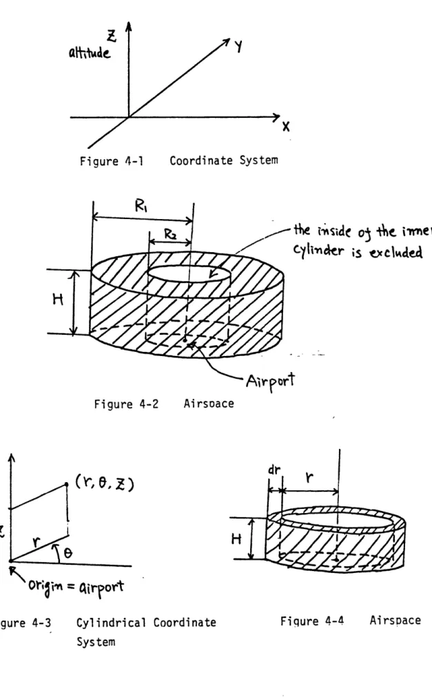
The results in this paper can be applied to evaluate the frequency of conflicts as well as that of collisions. In this paper, an aircraft is represented as a circular cylinder, and a collision is described as an overlap of two cylinders. If the size of the cylinder is expanded

to the volume of the protected airspace of an aircraft, an overlap of two cylinders means a conflict. Therefore, with a slight modification,

the results can be used to analyze the frequency of conflicts. This flexibility gives the models of this paper an important potential for application to a future air traffic control system. The FAA is currently developing a new type of air traffic control system called AERA (automated en route air traffic control). AERA is expected to reduce the workload of human controllers and expand the capacity of airspace using new computer systems and better communication links. When this system is fully implemented, aircraft will be able to fly under

the frequency of potential conflicts the computer system should handle becomes high. Therefore, the frequency of potential conflicts under various circumstances should be calculated in order to estimate the computer workload before full implementation of the system. The models

developed in this paper may be helpful in this evaluation.

The consequences of actual collisions are, of course, grave.

Fortunately, the average number of such collisions per year has remained

relatively small. According to an FAA Report (Report of the FAA Task Force on Aircraft Separation Assurance, Jan. 1979), the average number-of midair collisions reported to NTSB from 1974 through 1978 was 33 per year. Most midair collisions have occurred between small general aviation

aircraft operating under VFR. However, the report also states that there were 227 near midair collision reports in 1975 alone, and that air

carriers were involved in 68 of these cases. (According to the report, a near midair collision is an incident which would probably have resulted in a collision if no action had been taken by either pilot. Closest proximity of less than 500 ft would usually be required for a near midair collision report.) Although the number of conflicts is not available in the report, it is clearly far greater than the number of near midair collisions considering the difference of airspace volumes involved.

The outline of this thesis is as follows. In Chapter 2, we present an overview of two aircraft collision models, the Reich model and the gas model, which have been the most important ones in this field. In Chapter 3, we develop some extensions of the gas model including a generalized two-dimensional gas model, an overtaking model and a three-dimensional gas model. In Chapter 4, we develop an aircraft collision model which does not assume the uniformity of aircraft distribution. The conclusions of this thesis are summarized in Chapter 5.

CHAPTER 2

AIRCRAFT COLLISION MODELS

In this chapter, an overview of the Reich model is first presented, and then the gas model is briefly described. These models have been

the most important ones in estimating collision risks.

2.1 The Reich Model

Many models have been developed to estimate aircraft collision rates under various circumstances. Probably the best-known among them is the Reich model which was employed to assess the collision risk to flights over the North Atlantic Ocean as part of efforts to reduce the lateral separation between North Atlantic air routes.2,3

In the Reich model, an aircraft is represented by a box,, and a collision is described as an overlap of two boxes. The occurrence of this overlap is equivalent to the event that a point enters a box which has dimensions twice as large as those of the original box.

The collision rate is expressed as

-

1,Xt

FY -t-

Yy jz,(

where

is the expected frequency per unit of time with which the along-track separation shrinks to less than

.x.

and E are similarly defined.

is the probability that the along-track separation is less than K at a random instant of time.

VI

Model of Collision

V2

Oe

If we are calculating the collision rate between a pair of aircraft assigned to the same flight altitude and flying on parallel flight tracks separated by the lateral separation S Y , (2-1) becomes

FX Py (SY) P'

(0)

?

(

y)

-yO

( )ZP(0)

Py(s,)

seperation S, , is less- than 1y .

j(0) is the probability that the across-track separation between a pair of aircraft, assigned to the same track, is less than

(s)

is

the expected frequency per unit of time with which the

across-track separation between a pair of aircraft, nominally spaced at the lateral standard separation , shrinks to

less than Xy .

O') is the expected frequency per unit of time with which the

across-track separation between a pdir of aircraft, assigned to the same track, shrinks to less than

P

(0)

(

If aircraft on the same track are spaced with the along-track

separation _,

5x

and,

where

X

E,(o)

(D)

(0)

0z()

=

40/

0)

= 0.26

can be calculated if the probability distribution for the lateral deviation of aircraft from the center line of the track is known.

_PY(Y)(2-4)

where

f(y)

is

the probability distribution of lateral deviation of

aircraft from the center line of the track.

T(y) is estimated through the first Laplacian distribution.

Fz _V-2(2-5)O

where

G\ is the standard devaition, and is the mean of lateral

deviation.

Ty

(Sy)

=

EC

Py

F(Sy)

is the relative across-track velocity of a pair of aircraft. This completes a brief mathematical description of the Reich model. This model was employed to estimate the collision risk to flights over the North Atlantic Ocean in the 1960's. The number of flights over the North Atlantic Ocean increased dramatically in the 1950's and the early 1960's, and the traffic became seriously congested by the mid-1960's. The lateral separation between the center lines of adjacent air routes over the North Atlantic Ocean was 120 n.m. at that time, and the airlines

suggested thatthe lateral separation be lowered to 90 n.m.. The FAA agreed with the suggestion, and ICAO adopted it. However, airline

pilots were strongly against it, and the separation standard tentatively returned to the 120n.m. standard as a result of a hearing. Then the

study of the collision risk over the North Atlantic Ocean started. First data for lateral deviation from the center line of the air route were collected through the use of radars on land and on ships. Then the collision risk was determined using the Reich model. The conclusion was that the lateral collision risk at 90n.m. lateral separation was

about six times a great as at 120 n.m. separation. It also became obvious that the. lateral collision risk far exceeded the risk of collisipn with

one's vertical and longitudinal neighbors.

The final solution to this

problem was what is called staggered separation which is shown in

Figure 2-2,

Iatel seratio-n) /2 -"i77

~,ooo~t

Quo

Conventional Separation and Staggered Seoaration

Figure 2-2

risk over the ocean. Some more recent studies have attempted to estimate the collision risk to continental flights. Polhemus and Livingston

collected data for lateral deviations of aircraft flying in the VOR airways system.4 They concluded that the deviation distribution varies considerably with position with respect to the VOR. Based on this data, Polhemus calculated the collision rate of aircraft flying on two parallel air tracks within the VOR system.5

2.2 The Gas Model

Another well-known collision model is the gas model. The reason for this name is that its basic concept is essentially the same as that of a gas molecular collision model. A brief description of the two dimensional gas model is given below, and the generalized gas model will be developed in Chapter 3.

The two-dimensional gas model assumes that N aircraft operate in an area A. Each aircraft i, travels in a straight line with velocity

Vi, and direction distributed uniformly between 0 and 27T. Aircraft are uniformly and independently positioned over A.

The magnitude of the relative velocity of two aircraft i and j, is

Vr;

(vvi

ik~()

(2-7)

where

Vrii

j.

(3

probability of a collision between i and j during a period of time t is given by

El

2-5

Vr;ij

_(2-8)

A

If

E\Vr

H

2g E~y)

t

2

_z

A

_A

E(2-9)

In a three-dimensional problem, (2-9) gives the number of horizontal overlaps during a period of time t assuming that aircraft are flying

only horizontally. If the traffic density is uniform in an altitude layer

H thick, and an aircraft has the vertical dimension h, then the

three-dimensional collision rate can be obtained by multiplying (2-9) by

H-This model has been used to estimate the collision rate in terminal area.6,7 In reference 7, Flanagan and Willis developed a three-dimensional

gas model which allowed aircraft to have a vertical velocity component as well. However, this model assumed that directions of aircraft velocity are randomly distributed over three-dimensional angle. This assumption

is obviously unrealistic because airplanes do not have the capability to fly vertically like helicopters.

The gas model described above can deal only with simple cases. In the next chapter, the gas model is extended to a generalized form, and

the probability distributions of aircraft direction and altitude are analyzed in connection with the collision rate.

CHAPTER 3

SOME EXTENSIONS OF THE GAS MODEL

Some extensions of the gas model are presented in this chapter. First, a generalized two-dimensional gas model is developed. Then, the definition of expected relative velocity is examined, and some special

cases are analyzed. The overtaking problem is briefly discussed as a

special case of collision. The horizontal overlap rate and the proba-bility of vertical overlap are also discussed. Finally, a three-dimensional gas model is developed.

3.1 Generalized Two-Dimensional Gas Model

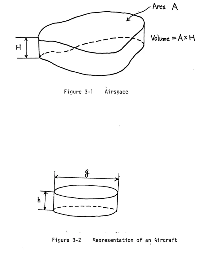
This model assumes that N aircraft are flying in the volume with

horizontal area A and height H (Figure 3-1).

Horizontally, aircraft are uniformly and independently distributed, and vertically, they are independently but not necessarily uniformly distributed. The horizontal distribution and the vertical distribution are independent of each other. All the distributions in this model are time-invariant. The assumption that the density of aircraft is time-. invariant can be justified considering that the collision rate is small and so is the rate of aircraft loss.

Each aircraft travels only horizontally. It is not assumed that each aircraft travels only in a straight line. No collision avoidance maneuver is taken, however. The assumption of no collision avoidance maneuver is obviously not realistic, and leads to an overestimated collision rate. However, as explained in Chapter 1, with a slight modification, the rate of conflicts can be calculated under the same

16

-Area

A

Figure 3-1 Airspace

Reoresentation of an Aircraft Figure 3-2

assumption, and that rate may be helpful in

estimating the workload of

pilots and air traffic controllers in

avoiding conflicts. Therefore, the

result with this assumption may be useful both in

obtaining a conservative

estimate of the collision rate and in

estimating the workload of pilots

and air traffic controllers in preventing collisions.

Each aircraft is

represented as a right circular cylinder, shown

in

Figure 3-2. A collision is

described as an overlap of two cylinders.

The occurrence of this overlap is

equivalent to the event that a point

representing a center of one aircraft enters the cylinder of another

aircraft which is

twice in

length and eight times in

volume as large

as the original aircraft (Figure 3-3).

The

collision rate is

expressed as follows.

C

TH XP

(3-1)

where

= the rate of collisions per unit of time

= the rate of horizontal overlap per unit of time

= probability that two aircraft overlap vertically given they overlap horizontally

= P (vertical overlap/horizontal overlap)

Horizontal overlap means that, neglecting the vertical axis, the horizontal coordinate of the center of one aircraft enters within a range of g from the horizontal coordinate of the center of another aircraft (Figure 3-4). Vertical overlap is similarly defined.

Let us consider

P,

first.

Collision Volume

Horizontal Overlap Figure 3-3

of aircraft,

Pv

VertieW\

overtoA

jor

tw

Aircrat)

Let (Z) be the probability density function for the altitude of aircraft.

f

)dz

is

flying at an altitude between

Z

Py

=I

_C;

du d

where G is the altitude of the lowest surface of the airspace under consideration.

Let us calculate

H

0

Crttj1(i

for the uniform

(Z)

Otherw/ise,

2h

H

- hz

If H >> h, then

.2h

This shows that if aircraft are uniformly distributed over an altitude layer H, with H much greater than the aircraft height h, the collision rate is approximately

Next, let us consider the rate of horizontal overlap Tl . As explained earlier, a horizontal overlap takes place when the center of an

Ade

CT

rovP

Figure 3-5

.,V

At

Vertical Overlao - -

-Execded

-numbr

og akta&t

9S e4

=

Horizontal Overlap in dt Figure 3-6

aircraft enters within a range of g from the center of another aircraft.

Let

E(\r)

be the expected relative velocity. Then, during a very

short period of time

dt

, each aircraft encounters

.2.1

(Vr)cit

f

overlaps on the average, where

I

is the horizontal density of

aircraft.

Since is N/A and there are N aircraft, the total number of

horizontal overlaps in dt is

Ix six

(2

_E(r

_tX

A

The reason for the multiplier 1/2 in (3-5) is that each overlap would otherwise be counted twice. Then,

H

_A

F(3-6)

From (3-1), (3-3) and (3-6), the collision rate is

C

A

EVr)

)

(3-7)

where

C = collision rate per unit of time

A = horizontal area of the airspace under consideration

G = altitude of the lowest surface of the airspace

G + H = altitude of the highest surface of the airspace

N number of aircraft in the airspace

g = horizontal dimension of aircraft

(,

NO= expected relative velocity

= probability density functipn of altitude of aircraft

If aircraft are uniformly distributed over altitude and

(3-8)

Below and in Section 3.3, we shall calculate

EN

)

E(Vr)

_V,

V

V,Vj-

2 V Vz t-0

)

where

/y.

(S

Then,

v,4v-y)V,

V((3)

f

(v)vA)c3

AVAvy

(3-lo)

where

= probability density function of

v)

probability density function of V

'23

0 and 27(, and the magnitude of velocity is constant,

Z

TG

O

'<2

7L

Then,

E (Vr)

=

(v"-

_1v'

_cosp)

_dI

.~ALVD

[Numerical Example]

Twenty aircraft are flying in the airspace shown in Fiqure 3-7. Each aircraft is flying horizontally at 300 kt in a random direction. Aircraft are represented by a circular cylinder with diameter of 150 ft.

and thickness of 50 ft. Aircraft are uniformly and independently distributed in the airspace both horizontally and vertically.

-4

Vo

=382

kt

2h

H

I00

A

=0.31n/

(3-11)

P

.

Figure 3-7

-Are4 =

oYxiol

=

Figure 3-3 Collision Rates in Different Areas ID.Qk

This may seem surprisingly large. This is

because the expected

relative velocity is

large in

this case.

3.2

Expected Relative Velocity

A brief discussion of the meaning of "expected relative velocity" will

be useful at this stage. It

seems simple at first to define the expected

relative velocity. However, the concept creates some difficulty in

estimating the collision rate in

the gas model. For simplicity, only

two-dimensional problems are dealt with in

this section.

It

is

sometimes maintained not only in

the field of air traffic

control

but also in

the field of statistical mechanics

that the collision

rate is given by the following formula

N(N-

I)

2$E

_(Vr)

C

.

A

(3-12)

2

A

where

E

r)

is

the expected relative velocity taken over all

possible pairs of aircraft. This equation is

different from (3-6), which

uses as its first term. If we are dealing with molecular collisions, N is a very large number and the difference between the two formulae is very small. Therefore, there is no practical problem in that field. But, in the case of aircraft collisions, the difference

may be of some

significance as the density of aircraft is

usually low.

We shall discuss the difference between the two formulae below.

El _______

pair of aircraft will meet each other during a very short period of time dt is

2a

E'Cv)

ct

there are KI(N- I

A

2

2~.'61t )dt

number of collisions during dt is

A

Therefore, the collision rate is given by (3-12).

Let us assume, at first, that (3-12) gives the correct collision rate.

Consider the situation shown in Figure 3-8. Suppose that there are M aircraft in the large area (10 1 x l0Q.) and the probability

distribution for the position of each aircraft is uniform over the area. The expected number of aircraft in the small area (kxk) is . Let us

calculate the two collision rates in the large area and in the small area. According to (3-12), the collision rate in the large area L is given

by *

CL-

M(

-v))

(3-13)

Similarly, the collision rate in the small area is

S

(3-14)

Since the large area can be sub-divided into 100 small areas,

CL

be 100 times as large as S . However,

_ 00 _ v D__ i a

'(W)

z

100ok

Then,

This is a contradiction. The explanation for this contradiction lies in the definition of the expected relative velocity

(Vr)

In (3-13) and (3-14), it is implicitly assumed that E'(Vr) is the

-same in

both areas. But

E(\r)

is

a function of N if

we are to

use (3-12).

E'(Vr)

in (3-12) is the expected relative

velocity taken over

all possible pairs of aircraft. Therefore, if

the number of aircraft

changes, so does 'E(Vr) . In order to make this problem clear,

let us consider some examples.

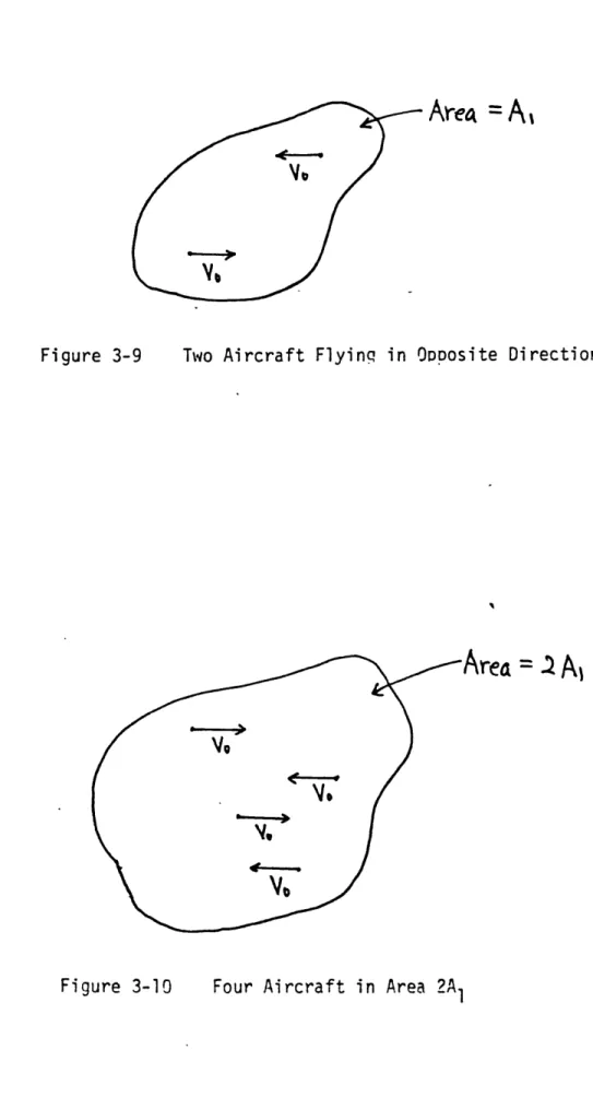
Suppose that two'aircraft are flying in opposite directions at speed

V

A,

and

(v\/.)

is

l2fV

The collision rate is given by (3-12).

2

A,

4t Vo

Next, suppose that four aircraft are flying at speed

"o

area . . Two of them are flying in the same direction, and the

other two are flying in the opposite direction. The probability

distribution of their positions is uniform over the area (Figure 3-10). is defined as the expected relative velocity taken over all possible pairs aircraft. Viewed from any one of the four aircraft, two other aircraft are moving at speed 1V, and the other one is

Area =

A,

Figure 3-9 Two Aircraft Flyinq in OpDosite Directions

=.2

A,

Four Aircraft in Area 2A₁ Figure 3-10

2V6tVO

+

4VO

3

3

This value is different from

E(Vy)

N(N- 2a E'vt

.2

_l

-

- ,

-

(

3

-1

9

)

2ZAi

A,

Therefore, the collision rate in the area : is twice as large as

the collision rate in the area A,,

These examples show that .'(Vy) , which is defined in (3-12) as the expected relative velocity taken over all possible pairs of aircraft, is a function of the number of aircraft. Next, the relation between

E(Vr)

and the mathematical expression for

E'(/r)

E()

E(v)

~

V

-Vi

\T( )

)

ddV

(3-20)

= velocity vector of aircraft i

= probability density function of velocity vector Let us calculate the average relative speed based on (3-20).

Suppose that there are N aircraft, and aircraft i has the velocity

vector \. . Then, the average relative velocity is

\

- \

(3-21)

However, the average relative velocity taken over all possible pairs of aircraft, which is defined as , is

- _{. (3-22)}

Since

-

0

,(3-22)

becomes

\

)(3-23)

N

-Therefore, if the expected number of aircraft is N(N

>

relation between f(V,') and is as follows.

N

\/y)

where

£(Vr) = expected relative velocity defined by (3-20)

= expected relative velocity taken over all possible

pairs of aircraft

Therefore, (3-6) and (3-12) used in this way give the same collision rate.

The reason for the difference between

E(Vy.)

and

5(/r)

is that

Let us examine the difference between and in the examples shown in Figure 3-9 and 3-10. \ in Figure 3-9 is

tIr

whereas

The collision rate in Figure 3-9 is

C =

_z

Ai

laVO _41V,

This is the same as (3-17).

The collision rate in Figure 3-10 is

-N

W

Z

A

2.Ai

At

This is the same as (3-19).

These examples show that EL'(Vr) is a function of the expected number of aircraft. If this fact is recognized; the formula

2N

2-a E'(v)

2

A

fact has been overlooked in the past in using the formula, and it is

inconvenient to use

E'(Vr)

F(V,)

expected numbers of aircraft. Therefore, from now on the preferred

iN

E(Vr)

formula

()

A

N(04-1)

_{.A ETVO )}

2

A

rates in this paper.

3.3

Special Cases

will be used (and

1 not be used) to estimate collision

The gas model developed by Graham6 and Flanagan7 assumes that

directions of aircraft velocity are uniformly distributed between 0

and

(3-26)

21(,.[see

one because destinations of aircraft are not uniformly distributed. In this section, the general formula for the collision rate for non-uniform probability distributions of aircraft direction is developed, and the collision rates for constant velocity (i.e., for when the

magni-tude of velocity is constant) are calculated for some special

distributions of aircraft direction. Some numerical examples for cases in which the magnitude of velocities is a random variable are also given.

The general formula for the collision rate is given by (3-7).

C

A7(Z)

(3-7)

where

= directional angle of velocity of aircraft i

= magnitude of velocity of aircraft -i

- = probability density function of G

=probability density function of

V/

The collision rate for any distribution of direction and magnitude of aircraft velocity is given by (3-7) and (3-28).

We calculate first the collision rate for constant velocity (the magnitude of aircraft velocity is constant).

Suppose that the magnitude of aircraft velocity is a constant Then,

2 VO

E(

(96)2

(3-29)

0

E(vr)

direction is tabulated in Table 3-1. It is assumed that horizontally aircraft are Uniformly distributed. The corresponding collision rate is given by (3-7). If positions of aircraft are uniformly distributed over altitude and the height of aircraft is negligibly small compared with the thickness of the altitude layer under consideration, the corresponding collision rate is given by (3-8).

A

For distributions other than the uniform vertical distribution, the collision rates can be calculated numerically.

Table 3-1 shows the values of the expected relative velocities for

some interesting probability density functions of velocity direction. For example, the third case in Table 3-1 is the one in which a fraction K of aircraft are flying in the same direction, while the directions of

the other (1 - K) fraction are uniformly distributed over 0 and .27.

In the fourth case, aircraft are flying only in two directions.

Table 3-1 shows E(Vr) only for the cases when the magnitude of the velocity is constant. If the magnitude of velocity is a random variable,

Expected Relative Velocity

e~Lo

( ) vI = constant)

Tabl e 3-1

00

e d

*)

S

(0) is

Ane Adtt

ito-n

35

[Numerical Example]

We now illustrate these results through numerical examples: assume

that 20 aircraft are flying horizontally in the airspace shown in

Figure 3-7. Each aircraft is represented by a circular cylinder with a

diameter of 150 ft. and a thickness of 50 ft.

3.3.1 Example 1

Aircraft are uniformly distributed over altitude. All aircraft are

flying in the same direction and at the same velocity.

E (V )

=

0

C(~)

0

C

(

colhsio,

rcte)

=0

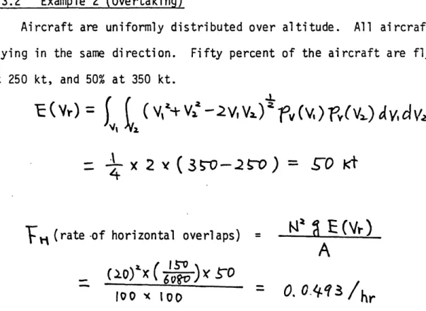
3.3.2 Example 2 (Overtaking)

Aircraft are uniformly distributed over altitude. All aircraft are

flying in the same direction. Fifty percent of the aircraft are flying

at 250 kt, and 50% at 350 kt.

"E

(Vr

(,

V -V, V2.),2f

V

(v)f

dy, d

x

2

(35--2

)

=

gO kt

-4

M*3

N(r)

(rate

-of horizontal overlaps)

A

oo

0-.

04-3/hr

V (probability of vertical overlap) 2.

I

0 0

2H

H

4.13

x

/r

(The overtaking problem can be treated as a special case of the

generalized collision problem. A brief discussion will be presented in the next section.)

3.3.3 Example 3

Aircraft are uniformly distributed over altitude. aircraft velocity are uniformly distributed over 0 a

Directions of nd 2T% . Fifty

percent of the aircraft are flying at 250 kt, and 50% at 350 kt.

COs ()X tx (,v)

r(v2.)

dc

a

VdV

is relative directional angle of velocity) 1

4 x

2-0

I

4-~

U

If

-4x

3S-50 - l-x33py.)30 x Coys

= 389 (this integral is numerically calculated)

VE

l

~-

4

0

X,

x ?v

(V4i-V

- V,

V,

A

1.10fx

3L

x

=

0.1%4

3.84

xK

10

/h,

3.3.4

Aircraft are uniformly distributed over altitude. Directions of aircraft velocity are uniformly distributed over 0 and llL. Magnitudes of aircraft velocity are uniformly distributed over 250 kt and 350 kt.

3Q 50 C

v,

2S

."

0.vt

= 384 (this integral is numerically calculated)

N

E(Vr)

T.

A

(20)xc

(IS

)X384

100

x

100

FE NV)

\00

x

C

too

'

I0 0

3.11 x

=0

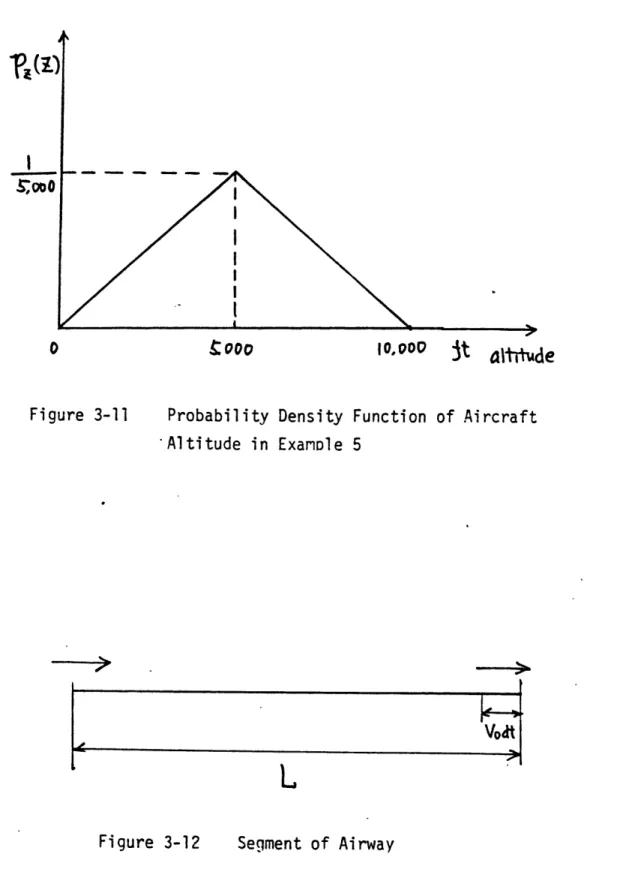
3.3.5 Example 5

The probability distribution of aircraft altitude is triangular as shown in Figure

Example 4.

\0,000

?V

3-11. The other assumptions remain the same as in

S. 10,000 \00 is the same as ~rzzcz in Example 4.

5.05

x

I(

/

~(z)

P7

(dA

av Az

/

7

5-= T" x ?v

0

t

000

Figure 3-11 _{Probability Density Function of Aircraft} Altitude in ExamDle 5 Segment of Airway 1, 411,1, d, 611, , wl"11WO14111kilim HINHIII 111110 S;000

10,000

it

tid

3.4 Overtaking

The overtaking problem in which aircraft are flying on a single route but not at the same velocity can be treated as a special case of the

generalized collision problem. Suppose that aircraft are flying on an airway. For simplicity, the width of the airway is assumed to be zero.

Then, the collision rate is the same as the overtaking rate. In this case, the expected relative velocity is

V, -

Val

V, V

Let us calculate the overtaking rate within the segment L of the airway, assuming N aircraft are uniformly and independently distributed

over the segment.

~T

=~E

(v)

where

T = overtaking rate within the segment L of the airway N = expected number of aircraft within the segment L of the

airway

It should be noted that the probability density function of velocity ?,(V) is defined here in the domain of space. In other words,

if one aircraft is randomly picked up from the airspace at a certain moment, the probability that its velocity is within V and V + dV

is

given by

ry(v) dv

.

If

fy(V)

is uniform between

\y,

and

between

V,

Va--

dy

VZ

which enter the segment. Let

ty(V)

function for the velocity of each aircraft entering or departing the

segment. Let us consider the short portion

VqO~t

segment (Figure 3-12). The expected number of aircraft with velocity

range

V

and

VtdaV

in this portion is given by

X

- -

yJ

Y

,

(vo) d

v

(3-32)

During the period of time dt, these aircraft will depart the segment. Then, the expected total number of aircraft departing the segment ...uring dt is given by

N

a

akdt

7VS

ayt(Yo)4VP

(3-33)

where / is the expected number of aircraft entering or departing the

segment during one unit of time.

Since the expected number of aircraft with velocity range \/Q and

V

4V

which pass the end of the segment during dt is given by

(3-32),

_Jy

_dt

dV

-

t,(v)dv

=

d

vlj~1

dl

Y()(3-34)

T

V

rf

yV i

T~

N(

-T~

'(v)dv)

.

I V,

_-

--

_VX

v

_V

(V)Vw\e cV

_(V,)

_dV,d

_{a 2}

2L

_Vi

_v

IV(Vy_

vvd

v2

2

,

y

V

, ya

When the overtaking rate is calculated, we should recognize which

probability density.function is given. If

1y(v)

is given, (3-30)

and (3-31) should be-used. On the other hand, (3-35) gives the overtaking

rate when

I

is employed.

1Oy(v)

is defined in the domain of

space, whereas -1y(V) is defined in the domain of time. In order to

illustrate the result of this section, a numerical example is presented below.

[Numerical Example]

The probability density function of velocity defined in the domain of space, py(y) is uniform from 200 kt to 300 kt.

y

=

.00.

V

300

0

otherwise

Aircraft are uniformly distributed along an airway, and the expected number of aircraft is 1/10 n.m.

From (3-31), the overtaking rate within a 100 n.m.-segment of the airway is

ago

-Fx-10-~j--

-V.

xy

200

a.oo

43

Next, the overtaking rate is calculated using (3-35).

v(v)

5

v

ey(V)

V

9

v

xtoo

K

-+i:

IV,-V-21

V,

V V

X2,

X

_25,000

dv,

dv,

This value agrees with the value by (3-31).

3.5 Probability Density Function for the Direction of Aircraft Which Maximizes the Collision Rate

Assuming that aircraft are flying horizontally and that the density of aircraft is uniform, the probability density function which maximizes

the collision rate is the uniform probability density function between 0 and 27E . In other words, collisions happen most frequently when

destinations of aircraft are uniformly distributed, assuming the density of aircraft is uniform. The proof of this statement is presented below.

Since the collision rate is proportional

E(Vt/)

the

probability density function for aircraft direction which maximizes

E(V)

Let ₉₁

aircraft and

& and(

.S

/ , be the directional angles of velocity of two

the angle between the two vectors (Figure 3-13).

and -

()

is given by

1%(O

±~g)de

S7

For convenience of calculation,

~e)

J~

Then, _{( )}

1F'

(Q)

Vr)

is also defined as follows

0&9

<

IT

(3-37)

(3-38)

ro

(0

)

by

T'O

w3P1V(Vi)

£)

dVdV.,

Let us examine Since _(' has a cycle of ..TL ,

it can be expressed as a Fourier series.

01i

-E~)

,

( )

-(0)

V,

0 .6<

4TL

.7m

(c

± )

03Co's3

(v,) &(V2)dVdIV

V

V24v.vV,

c

-Cos

( .

(

Q

ts

n

QO

E

(VIr )

)(0)

Cos

-n\6

dG

r(o) siY\ -no A19

(n, cos v9+6,si-n no)

271L Op

FO (0)

0

(i )W

tU

(Q[

)1

(VAPlvyo

0

It can be shown that

\

\s

n

(

is always

negative for any set of positive values of

-n , \, OQA

V

The proof

is given in Appendix A. Then,

E

(Vr)

is

maximum when

and

are zeroes for all n. This means that

E(Vr)

is maximum when

1e(e)

=

%:i

From (3-37) and (3-40),

( ::.. .- ~0 L (Cl0 t:5TYi)

0 9<.T,(-44)

(3-45)

This result may be contrary to our intuition.

It would seem that

if

50% of aircraft were flying in

the same direction and 50% in

exactly

the opposite direction, the expected relative speed would be maximum.

This is

not true, however, because among each 50% of the aircraft flying

If the magnitude of velocity is constant

V

V

for the uniform distribution of direction is * Therefore, the

collision rate becomes maximum when directions of aircraft velocity are

uniformly distributed between 0 and 17 .

(NOTE) If directions of aircraft are discrete, the probability density

function of

%(p)

consists of impulses.

For example, when 50% of

9

=

=

0

=

expressed as a Fourier series. However, eveni if such cases are

considered, the uniform continuous (not discete) probability distri-bution maximizes the expected relative velocity. In other words, the uniform probability distribution (the probability density function is

between 0 and D76) maximizes the expected relative velocity

for any continuous and discrete probability distributions. The proof is given in Appendix B.

3.6 Probability of Vertical Overlap

The collision rate is given by (3-1) and (3-2).

CH

(3-1)

where

C

FH

The maximization of F, was discussed in Section 3.5. In this section,

Py

Py

C,

-where

= probability density function of altitude of aircraft

h

= lowest altitude of the airspace under consideration

Ct

H

I-

If H

>>

h

within an altitude

can be regarded approximately constant range 2h, PV can be approximated by

?z(Z)

d

Z

Through this approximation, it can be shown that the probability of vertical overlap becomes minimum when aircraft are uniformly distributed over altitude.

SA

If

(

)R

Is

p

)

-W~z~~

1

hI

C-4

-t Vi

pz(u ) 4w dz

) (Fa oo

From (3-47), (3-48) and

(3-49),-Gto

(3-50)

Then,

CA

4(3-51)

It is obvious that the probability of overlap is maximum

(

?v

=

)

when the vertical distribution of aircraft is concentrated within the altitude range h. (All aircraft are flying with altitude between

Zo

and Z, *

.)

The result that the probability of overlap is minimum when the distribution of aircraft altitude is uniform contrasts with the result

in Section 3.5 that the horizontal overlap rate is maximum when the

distribution of aircraft velocity direction is uniform. However, this is not a surprising result, intuitively.

51

3.7 Collision Rate between VFR Aircraft and Aircraft on an Airway

So far, collision rates have been calculated for one type of aircraft.

In other words, it has been assumed that all aircraft have the same probability distribution with respect to velocity, direction and space. In this section, a special case of collision between two different types

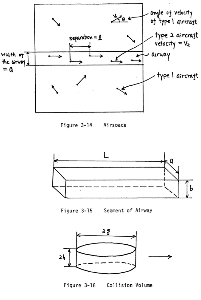
of aircraft is analyzed. Consider the situation described below. Assume that there are two types of aircraft. Type 1 aircraft are similar to the aircraft which have been analyzed so far. In this section, it is further assumed that type 1 airciraft are uniformly and independently distributed in the airspace. (In Section 3.1, uniformity is assumed only horizontally.) Type 1 aircraft can be regarded as

"VFR aircraft".

Type 2 aircraft are flying on an airway at constant

velocity, and in a direction parallel to the ainay. They are flying at a constant separation distance t from each other (see Figure 3-14).

The expected relative velocity of type 1 and type

2

aircraft,

is then given by

where

VI

V

=

angle of direction of type 1 aircraft

( 9

0 in the direction of type 2 aircraft)

~v

(V )=

_{probability density function of}

_V,

Figure 3-14 Figure 3-15

ac&le

ol vdocrt

04

ijff

1

velocil = Va

,.- type

I

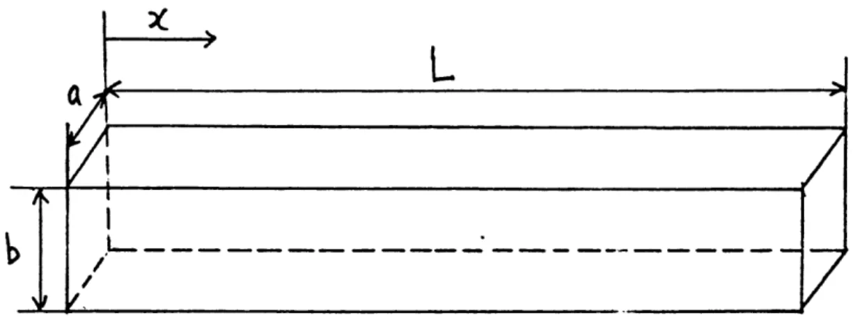
aircm-t

The width of the airway is a, and the thickness of the airway

(the altitude layer in which type 2 aircraft are flying) is b, as shown in Figure 3-15.

Each aircraft is represented as a circular cylinder with diameter g

and height h as before.

The occurrence of a collision is equivalent

to the event that the center of an aircraft enters the cylinder of another

aircraft which is twice in length and eight times in volume as large as

number of collisions one type 2 aircraft is expected to have during one

unit of time is the density of type 1 aircraft multiplied by the volume

which the cylinder moving at the expected relative velocity generates

during one unit of time (Figure 3-16).

The volume generated by the movement of the cylinder during one

unit of time is given by

4

3

h

E

(

vrm)

Then, the number of collisions one type 2 aircraft is expected to have during one unit of time is

4

1

h

E(Vr),f

where

aircraft in one unit of

volume.

Since there

are

L

_{type 2 aircraft within the segment}

L

_of

the airway, the collision rate is

4Th

L.PE(Vrix)

It should be noted that no assumption has been made with regard to the probability distribution of the lateral and vertical position of type 2 aircraft within the airway. The rate of collisions between type 1 aircraft and type 2 aircraft is thus independent of the

probability distribution of position of type 2 aircraft on the cross-section of the airway and the dimension of the airway (C is independent of a and b). The reason is that no matter where a type 2 aircraft is flying, the expected density of aircraft 1 and the expected relative

velocity are constant.

[Numerical Example]

Velocity of type 1 aircraft,

V,

Velocity of type 2 aircraft,

V

Horizontal dimension of aircraft, g, is 150 ft. Vertical dimension of aircraft, h, is 50 ft.

Length of the segment of the airway, L, is 100 nm. Separation of type 2 aircraft, I , is 10 n.m.

Density of type 1 aircraft is the same as in Figure 3-7.

(

f2O/

(o0,ooo-n-rn

x

lo,000 jt))

Directions of type 1 aircraft are uniformly distributed between

0 and

2TX.

Then

4h

LP

E(vrix)

=

3'~A'

x

1

3.8

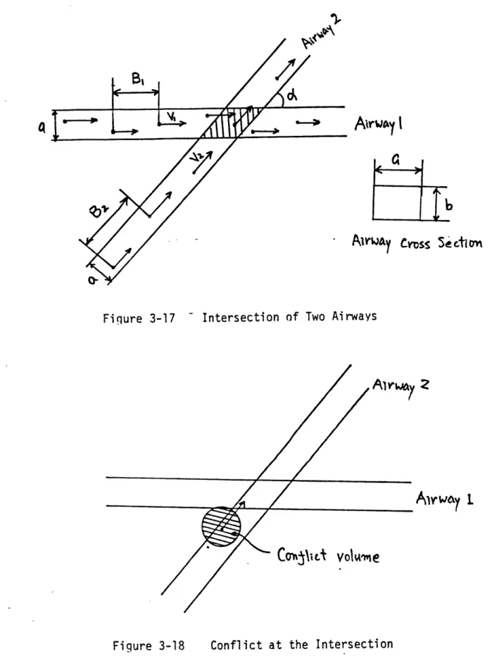
Collision Rate at the Intersection of Two Airways

In this section, we shall discuss the collision rate at the inter-section of two airways. Consider the two intersecting airways shown in Figure 3-17. Both airways have the same width a and the same

height b. The probability distribution of aircraft position on the cross-section is uniform. At first, it is assumed that aircraft on the same airway are flying at the same velocity and with the same

separation. The case in which separations between aircraft are given by Poisson processes will be discussed later. The separations on airway 1 and 2 are

t3,

on airways 1 and 2 are

\

and

V

respectively.

The angle

Consider one aircraft on airway 2 which enters the intersection shown as the shaded area in Figure 3-17. The expected number of aircraft on airway 1 which the above aircraft encounters during one unit of time

is given by

E

X

_(3-56)

B,ab

.

The first term of (3-56) represents the rate of horizontal overlap, and the second term is the probability of vertical overlap, assuming that a and b are sufficiently large compared with g and h which

/

A-trwoy I

CIA

Airway

Figure 3-17 - Intersection of Two Airways

Aiwa4

2

Aiwway

1.

Co-tbid

VolW'Me

Conflict at the Intersection

criOSS Sedici

is

constant and given by

(

y,

X+/2-

-

Cos

j

)

,

(3-56)

4 h

('v-+

Va'-

.

v

o

a

b

B,

The expected number of aircraft 2 in the intersection is given by

)( _(3-58)

61 B Sim a B, S i-A

From (3-57) and (3-58), the collision rate is given by

h~,+li~ts

Q

4

bVL

Vx -,

Basd

V _C(3-59)

6,

BB.

i'ied

This is the collision rate with fixed separations. Next, we shall discuss the situation in which separations between aircraft are given by Poisson processes. Aircraft on airway 1 enter the airway with velocity \/i according to a Poisson process with intensity

X

and are similarly defined. Then, the .average separations

on airway 1 and 2 are given by

V'

and

-

Since the two

processes are independent, the collision rate is given by (3-59)

substituting and- for BI and Then, the

collision rate is

4

h

X

,

Xz

(V2+ V2- -AV, Va.tos

d

b , v42 s

i-ya

More gnerally, the collision rate at the intersection is given by

4

C

(v

Va

IV,

VX Cos

_(3-61)

b

0E(8 F

(s8,)

-s

%n

d

where

'(E

)

consecutive aircraft on airway 1

"F )

It is assumed that the processes of aircraft flows on the two airways are independent of each other.

Section 3.7 and this section have dealt with the rate of collisions between two different types of aircraft. The general formula for these

cases will be derived in the next section.

[NOTE]

In Reference 9, Dunlay developed a conflict model which is similar

to the model in this section. However, there is some difference between the two models. First, the Dunlay model assumes that the width of an airway is equal to zero, which can be treated as a special case of the

model in this section. The second difference concerns the volumes

involved in a collision and in a conflict. A collision is described as an event in which the volume of an aircraft overlaps the volume of another aircraft.. A conflict happens when an aircraft penetrates the

outer surface of the protected airspace of another aircraft. Therefore,

as long as the density of aircraft is uniform in airspace, the rate of conflicts can be obtained from a collision model simply by making the

appropriate change for the volume involved. In the case of the

intersection problem, however, the density of aircraft is not uniform in airspace. Therefore, the collision model in this section cannot be directly applied to the rate of conflicts at the intersection because of the boundary problem (Figure 3-18). However, the rate of conflicts

can be deduced from the collision model in this section.

Consider a portion of the airspace shaped like a parallelogram with the length of a side

L

as negligibly small. The conflict rate in this case is directly

calculated from (3-61), substituting the dimensions of conflict for g and h. Let us consider the cases shown in Figure 3-20. First all the aircraft flying in one direction are concentrated on an airway parallel

to the aircraft direction.

Since the number of conflicts each aircraft on the airway is expected to have during one unit of time is equal to that of each aircraft flying in the direction in the original case (Figure 3-19).,

the conflict rates in both cases are the same. Next, all the aircraft

in the other direction are concentrated on another airway parallel to the aircraft direction. Since the number of conflicts each aircraft on the second airway is expected to have during one unit of time is the same as in the previous case, the conflict rate of the last case is the same as that of the original case. Then, the conflict rate at the

L

Fiqure 3-19 Parallelogram Airsoace

Equivalent Cases

original case is directly calculated from (3-61). It should be noted that no assumption has been made with regard to the probability distribution of cross-airway position of aircraft. Therefore, (3-61)

gives the conflict rate as well as the collision rate for any

probability distribution of cross-airway position of aircraft. The

result of the Dunlay model can be derived as a special case of (3-61).

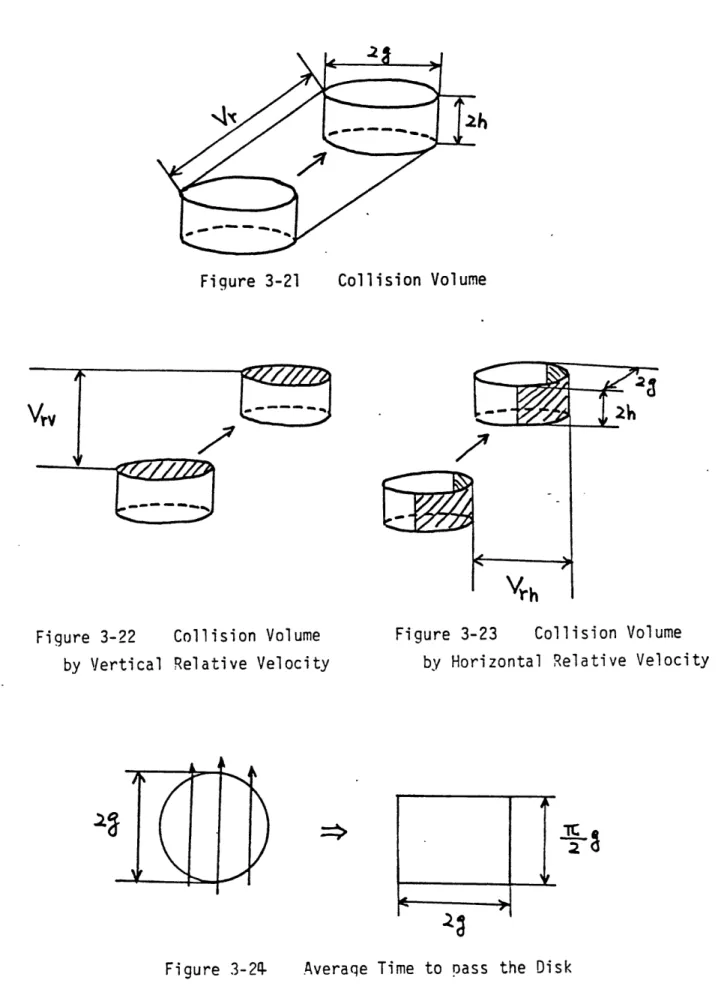
3.9 Three-Dimensional Gas Model - -

-So far, it has been assumed that each aircraft travels only

horizontally. In this section, the limitation is removed. The

three-dimensional gas model presented here assumes that N aircraft are flying in the airspace volume B. Aircraft are uniformly'and

independently distributed in the airspace. The vertical velocity and the horizontal velocity of an aircraft are assumed independent of each other. No collision avoidance maneuver is taken. Each aircraft is

represented as a right circular cylinder, as shown in Figure 3-2. It is assumed that this cylinder does not tilt even if its velocity has a vertical component,

A collision takes place when the center of one aircraft enters the cylinder of another aircraft shown in Figure 3-3. Therefore, the number of collisions an aircraft is expected to have during one unit of time

is the density of aircraft multiplied by the volume which the cylinder moving at the relative velocity generates during one unit of time.

Let

V

be the relative velocity.

Vrv

is

the vertical

relative velocity or the vertical component of

Vr

\/h