HAL Id: hal-01257078
https://hal.archives-ouvertes.fr/hal-01257078v2
Submitted on 22 Sep 2015
HAL is a multi-disciplinary open access
archive for the deposit and dissemination of sci-entific research documents, whether they are pub-lished or not. The documents may come from teaching and research institutions in France or abroad, or from public or private research centers.
L’archive ouverte pluridisciplinaire HAL, est destinée au dépôt et à la diffusion de documents scientifiques de niveau recherche, publiés ou non, émanant des établissements d’enseignement et de recherche français ou étrangers, des laboratoires publics ou privés.
programming
Jaime Arias, Michell Guzmán, Carlos Olarte
To cite this version:
Jaime Arias, Michell Guzmán, Carlos Olarte. A symbolic model for timed concurrent constraint programming. Ninth Workshop on Logical and Semantic Frameworks, with Applications (LSFA 2014), Sep 2014, Brasilia, Brazil. pp.161-177, �10.1016/j.entcs.2015.04.010�. �hal-01257078v2�
A Symbolic Model for Timed Concurrent
Constraint Programming
Jaime Arias
1Univ. Bordeaux, LaBRI, UMR 5800, F-33400 Talence, France CNRS, LaBRI, UMR 5800, F-33400 Talence, France
Michell Guzm´
an
2Com`ete, LIX, Laboratoire de l’Ecole Polytechnique associ´e `a l’INRIA/CORDI-S. France DECC, Universidad del Valle. Colombia
Carlos Olarte
3ECT, Universidade Federal do Rio Grande do Norte. Natal, Brazil DECC, Pontificia Universidad Javeriana Cali. Colombia
Abstract
Concurrent Constraint Programming (ccp) is a model for concurrency where agents interact with each other by telling and asking constraints (i.e., formulas in logic) into a shared store of partial information. The ntcc calculus extends ccp with the notion of discrete time-units for the specification of reactive systems. Moreover,ntcc features constructors for non-deterministic choices and asynchronous behavior, thus allowing for (1) synchronization of processes via constraint entailment during a time-unit and (2) synchronization of processes along time-intervals. In this paper we develop the techniques needed for the automatic verification ofntcc programs based on symbolic model checking. We show that the internal transition relation, modeling the behavior of processes during a time-unit (1 above), can be symbolically represented by formulas in a suitable fragment of linear time temporal logic. Moreover, by using standard techniques as difference decision diagrams, we provide a compact representation of these constraints. Then, relying on a fixpoint characterization of the timed constructs, we obtain a symbolic model of the observable transition (2 above). We prove that our construction is correct with respect to the operational semantics. Finally, we introduce a prototypical tool implementing our method.
Keywords: Concurrent constraint programming, temporal logic, model checking
1
Introduction
In the last years we have seen how Concurrent Constraint Programming [20,21] (ccp) has been extensively used to specify and program concurrent systems. The
1 Email: [email protected] 2 Email: [email protected] 3 Email: [email protected]
This paper is electronically published in Electronic Notes in Theoretical Computer Science
increasing interest in the community for this powerful model of concurrency is per-haps due to its simplicity and tight connection to logic: processes tell and ask in-formation (formulas in logic) in a store of partial inin-formation; moreover, processes can be seen as both computing agents and as logic formulas. The use ofccp models has pervaded different areas in science (e.g., biochemical systems), engineering (e.g., security protocols, mobile and service oriented computing and social networks) and even the arts (e.g., tools for multimedia interaction)–see a survey in [17]. Never-theless, in spite of the many semantic and logical frameworks designed to reason aboutccp processes, the automatic verification of ccp programs has received little attention so far.
This paper aims at providing the theoretical and practical tools to carry out the verification of systems specified in thentcc [16] calculus, a timed extension of ccp to model reactive systems. For that, we propose a symbolic representation of the behavior of processes and we prove that such symbolic model is suitable to be used as a basis for standard techniques in model checking. One of the challenges to define such symbolic representation is that the operational semantics of ntcc is given by two different transition relations: the internal transition representing the steps of the processes during a time-interval and the observable transition describing how processes evolve along time-units. Moreover, the proposed model has to deal with two non-elementary temporal constructs in ntcc: !P that executes infinite copies ofP (one per time-unit) and ?P that describes asynchronous behavior by delaying P an unbounded (but finite) number of time-units. As we shall see, we can neatly characterize the behavior of these constructs by means of a fixpoint computation.
Organization and contributions. We start recalling thentcc calculus in Section
2. Section3describes our approach to represent symbolically the behavior of ntcc processes. We prove that the symbolic model can be obtained for any process in a finite number of steps (Theorem3.6) and also that our construction is correct with respect to the operational semantics (Theorem 3.9). In Section 3 we also present some examples to show how to compute the symbolic model of a process. Section4
describes the logic that we shall use to specify properties and Section5 shows how the symbolic model can be used in standard (symbolic) model checking algorithms. We conclude in Section 6 by pointing out to related work and briefly describing a prototypical tool implementing our methodology.
2
The ntcc Calculus
Concurrent Constraint Programming (ccp) [20,21] (see a survey in [17]) is a model for concurrency that combines the traditional operational view of process calculi with a declarative view based on logic. This allowsccp to benefit from the large set of reasoning techniques of both process calculi and logic.
Processes in ccp interact with each other by telling and asking constraints (pieces of information) in a common store of partial information. The type of constraints processes may act on is not fixed but parametric in a constraint system (CS). Intuitively, a CS provides a signature from which constraints can be built from basic tokens (e.g., predicate symbols) and variables, and two basic operations:
conjunction (t) and variable hiding (∃). The CS defines also an entailment rela-tion (`) specifying inter-dependencies between constraints: c ` d means that the informationd can be deduced from the information represented by c. Such systems can be formalized as a Scott information system as in [21], or they can be built upon a suitable fragment of logic e.g., as in [10,16]. Here we shall follow the second approach and constraints are seen as formulas in intuitionistic logic.
Definition 2.1 (Constraint System) A constraint system is a tuple (C, `) where C is a set of formulas (constraints) built from a first-order signature and the follow-ing grammar
F := true| A | F ∧ F | ∃x.F
where A is an atomic formula. We shall use c, c0, d, d0, etc, to denote elements of C. Moreover, let ∆ be a set of non-logical axioms of the form ∀x.[c ⊃ c0] where all free variables in c and c0 are in x. We say that d entails d0, written as d` d0, iff the sequent ∆, d−→ d0 is probable in LJ [13].
2.1 Process Syntax
Thentcc calculus [16] extendsccp with time-units for the specification of reactive systems, i.e., systems that continuously interact with the surrounding environment. In this language, time is conceptually divided into discrete intervals (or time-units). Intuitively, in a particular time interval, a process P receives a stimulus (i.e., a constraint) from the environment, it executes with this stimulus as the initial store, and when it reaches its resting point, it responds to the environment with the resulting store. The resting point also determines a residual process Q, which is then executed in the next time interval.
Definition 2.2 (Syntax) ProcessesP , Q, . . .∈ Proc are built from constraints in the underlying constraint system as follows:
P, Q, . . . ::= tell(c)|P
i∈Iwhen ci do Pi | P k Q | local x(P ) | next P | unless c next P | ! P | ? P
Untimed processes. The process tell(c) adds the constraint c to the current store, thus makingc available to other processes in the current time interval. Let I be a finite set of indexes. The ask process P
i∈I
when ci do Pi non-deterministically chooses a processPi s.t. ci is entailed by the current store. The chosen alternative, if any, precludes the others. If no choice is possible in the current time-unit, all the alternatives are precluded from execution. Ask processes thus define a powerful synchronization mechanism based on entailment of constraints. For the sake of read-ability, we shall omit “P
i∈I
” whenI is a singleton and we simply write when c do P . The process P k Q represents the parallel composition of P and Q. The process local x(P ) behaves like P , except that all the information on x produced byP can only be seen by P , i.e., x is a local variable of P .
Timed processes. The process nextP delays the execution of P for one time-unit. We shall use nextnP as an abbreviation for next next · · · next P where next is repeatedn times. The process unless c next P is also a unit delay but the process
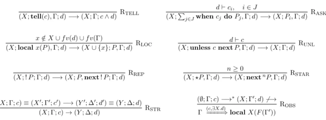
(X; tell(c), Γ; d)−→ (X; Γ; c ∧ d)RTELL d` ci, i∈ J (X;P j∈JwhencjdoPj, Γ; d)−→ (X; Pi, Γ; d) RASK x /∈ X ∪ fv(d) ∪ fv(Γ) (X; local x(P ), Γ; d)−→ (X ∪ {x}; P, Γ; d) RLOC d` c
(X; unless c next P, Γ; d)−→ (X; Γ; d) RUNL
(X; ! P ; Γ; d)−→ (X; P, next ! P ; Γ; d)RREP n≥ 0 (X; ?P, Γ; d)−→ (X; nextnP, Γ; d)RSTAR (X; Γ; c)≡ (X0; Γ0;c0)−→ (Y0; ∆0;d0)≡ (Y ; ∆; d) (X; Γ; c)→ (Y ; ∆; d) RSTR (∅; Γ; c) −→∗(X; Γ0;d) 6−→ Γ (c,∃X.d)====⇒ local X(F (Γ0)) ROBS
Fig. 1. Internal (−→) and Observable (=⇒) transitions. Let Γ = {P1, . . . , Pn}. The future of Γ, F (Γ), is
{FP(P1), . . . , FP(Pn)} where FP(
P
j∈Jwhen cjdo Pj) = ∅ and FP(next Q) = FP(unless c next Q) = Q.
The set of free variables in d (resp. P ) is denoted as fv (d) (resp. fv (P )).
P is executed in the next time-unit only if the guard c cannot be entailed from the current store. This is known as a negative ask or the preemption ofP .
The process !P represents unboundedly many copies of P but one per time-unit. This is, !P can be seen as P k next P k next2P· · · . This construct is powerful enough to encode some forms of recursive definitions inntcc as shown in [16]. Finally, the process ? P represents an arbitrary long but finite delay for the activation ofP . This process can be viewed as P + next P + next2P + . . ..
2.2 Structural Operational Semantics (SOS)
The SOS of ntcc consists of two kind of reductions: the internal transition (−→) representing the evolution of processes during a time-unit and the observable tran-sition (=⇒) representing the evolution of processes between time-units.
The internal transition relation γ −→ γ0 satisfies the rules in Figure 1. Here we follow the formulation in [10] where the local variables created by the program appear explicitly in the transition system and parallel composition of agents is identified as a multiset of agents. More precisely, a configuration γ is a triple of the form (X; Γ; c), where c is a constraint representing the store, Γ is a multiset of processes, and X is a set of hidden (local) variables of c and Γ. The multi-set Γ = {P1, P2, . . . , Pn} represents the process P1 k P2 k . . . k Pn. We shall indistinguishably use both notations to denote parallel composition of processes. Moreover, processes are quotiented by a structural congruence relation ∼= satis-fying: (STR1) local x(P ) ∼= local y(P [y/x]) if y /∈ fv(P ) (alpha conversion); (STR2) P k Q ∼= Q k P ; (STR3) P k (Q k R) ∼= (P k Q) k R. We shall write (X; Γ; c)≡ (X0; Γ0;c0) wheneverX = X0, Γ ∼= Γ0 and c≡ d (i.e., c ` d and d ` c).
The rules in Figure 1 are straightforward realizing the operational intuitions given above: a tell agent tell(c) adds c to the current store d (Rule RTELL); the process P
i∈I
whenci doPi executesPi if its corresponding guardci can be entailed from the store (Rule RASK); a local process localx(P ) adds x to the set of hidden variables X when no clashes of variables occur (Rule RLOC). Observe that rule RSTRcan be used to do alpha conversion if the premise x /∈ X ∪ fv(d) ∪ fv(Γ) does not hold; if the current store entailsc, then the process P in unless c next P is not executed (Rule RUNL); the seemingly missing rule for the process nextP is given
by the Rule ROBS as explained below; the process !P generates a copy of P and then, it is executed again in the next time-unit (Rule RREP); for a givenn≥ 0, the process? P executes nextnP (Rule R
STAR).
Let us now describe the rule for the observable transitions. Rule ROBSsays that an observable transition fromP labeled with (c,∃X.d) is obtained by performing a terminating sequence of internal transitions from (∅; Γ; c) to (X; Γ0;d), for some Γ0. The process to be executed in the next time interval corresponds to the future of Γ0 (i.e.,F (Γ0)) as shown in Figure1. Note that the future functionF is not defined for the processes tell(c), local x(P ), ! P and ? P since all these processes have an internal transition. Moreover, the variables in X are hidden by using existential quantification, i.e., the information aboutX is not visible from the final store d. Definition 2.3 (Observable Behavior) Let P be a process and s = c1.c2.c3· · · be an infinite sequence of constraints. We say thatP outputs s0 =c01.c02.c03· · · under inputs if P ≡ P1 (c1,c01) ====⇒ P2 (c2,c02) ====⇒ P3 (c3,c03) ====⇒ · · · and we write P (s,s 0)
====⇒. We define the input-output behavior of P as the set io(P ) ={(s, s0)| P ====(s,s0)⇒}.
3
Symbolic Model of ntcc Processes
Model Checking [6] (see a survey in [19]) is a well established technique for the automatic verification of systems. In this section, we show how to construct a symbolic, and then compact, model of the behavior of a ntcc process. Later, in Section5, we shall use this model as input to a symbolic model checking algorithm. One of the main difficulties to develop automatic verification techniques forntcc programs is the fact that the semantics of processes is given by two different tran-sition systems, namely, the internal (−→) and the observable (=⇒) transitions. On one hand, building a model for the internal transition seems to be unnecessary since the internal movements of a process during a time-unit are unobservable from the external environment. Moreover, abstracting away from the internal transition should lead to a more compact representation of the system, thus reducing the search space. On the other hand, the internal transition dictates much of the ob-servable behavior when non-deterministic processes are considered (see e.g., Rules RASK and RSTAR). Our approach is then to use (temporal) formulas as a compact representation of the reachable states (i.e., stores) of a process. As we shall see, the proposed formulas capture the observable contributions (i.e., constraints) that processes can make to the final store; additionally, the internal (unobservable) tran-sitions are symbolically captured by logical connectives. More precisely, we shall follow the steps below:
- Step 1: Give a logical interpretation of P (Definition 3.2). The interesting cases will be the temporal operators ! and? that require a fixpoint characteri-zation.
- Step 2: Perform a fixpoint computation to find a formula that models, sym-bolically, the reachable states of P .
S(tell(c)) = c S(P i∈IwhencidoPi) = V i∈I (¬ci)∨ W i∈I (ci∧ S(Pi)) S(P k Q) = S(P ) ∧ S(Q) S(local x(P )) =∃x.(S(P ))
S(next P ) = ◦(S(P )) S(unless c next P ) = (¬c ∧ ◦(S(P ))) ∨ c S(? P ) = µY.(S(P ) ∨ ◦(Y )) S(! P ) =νY.(S(P ) ∧ ◦(Y ))
Fig. 2. Symbolic representation ofntcc processes (Definition3.2). ¬c denotes the absence of c. - Step 3: Deal with dead-ends, i.e., states without any transition.
3.1 Step 1: Logical Interpretation of Processes
We start by introducing some needed notation. The behavior of a process will be specified as a disjunction of formulas of the shape
◦0(c
0)∧ ◦1(c1)∧ · · · ∧ ◦n(cn) (1)
where each ci is a constraint (Definition 2.1). Intuitively, the above formula reads as “c0 is valid in the current state and, afteri observable transitions, ci holds”. The “◦” symbol corresponds to the next modality in Linear Time Temporal Logic (LTL) [14] as described below. For the sake of readability, we writec instead of ◦0(c) and ◦(c) instead of ◦1(c). Moreover, we write
{{F1 1, F21,· · · , Fn11}, {F 2 1, F22,· · · , Fn22}, · · · , {F m 1 , F2m,· · · , Fnmm}}
instead of the following formula in disjunctive normal form
(F1 1 ∧ F21∧ · · · ∧ Fn11)∨ (F 2 1 ∧ F22∧ · · · ∧ Fn22)∨ · · · ∨ (F m 1 ∧ F2m∧ · · · ∧ Fnmm) (2)
Definition 3.1 (States) We shall use C◦ to denote the set of formulas built from the set of constraints C and the LTL operator ◦ (next). A state is a conjunction of C formulas of the shape c1∧ · · · ∧ cm. Two states A and B are equivalent if A` B andB ` A. A C◦ formula of the shape F = A
0∧ ◦(A1)∧ · · · ∧ ◦n(An) represents a label transition system (LTS) where there is a transition from state sx to statesy, notation sx ; sy, if Ai (resp. Ai+1) holds in sx (resp. sy). We shall use L(F ) to denote such an LTS. Given an LTS L, we shall use state(L) (resp. trans(L)) to denote the set of states (resp. transitions) of L.
Now we are ready to give logical meaning to processes by usingC◦ formulas. Definition 3.2 (Symbolic Representation) Given a ntcc process P , let S(P ) be inductively defined as in Figure 2 where µ (resp. ν) represents the least (resp. greatest) fixpoint operator in the complete lattice hL(C◦),≤i where L1 ≤ L2 iff state(L1)⊆ state(L2) and trans(L1)⊆ trans(L2).
Let us give some intuitions about the previous definition. A process tell(c) defines a state wherec holds. A processP
i∈IwhencidoPigenerates a state where none of the guards hold (V
i∈I
(¬ci)) and states where ci and S(Pi) hold. A process P k Q defines states where both S(P ) and S(Q) hold. A local process local x(P )
generates a state whereP holds but the information about x is irrelevant. A process unlessc next P defines a state where c holds (and then P is not executed) and a state wherec is absent (i.e., ¬c) and the states generated from P hold.
As shown in [16], the process ?P resembles the eventually modality (3) in LTL. Then, the states generated by this process can be characterized as the least fixpoint of the disjunction of a state whereP holds and a state where P holds in the next time-unit. Similarly, the process !P resembles the always (2) modality in LTL. Then, the generated states correspond to the greatest fixpoint of the conjunction of a state satisfyingP and a future state where P also holds.
3.2 Step 2: Fixpoint Computation
Once we have the logical readingS(P ) of a given process P , we need to perform a fixpoint computation in order to obtain aC◦ formula representing symbolically the states of the system. Before giving some examples of this step, we need to define the degree of a formula (Notation3.3below) and a simple program transformation in order to capture correctly the state transitions.
Consider the process P = next tell(c). We know that S(P ) = ◦(c). Then, what should be the observable behavior ofP during the first time-unit? We know that P does not add any information to the first time-unit. Then, we need to “complete” the formula ◦(c) to model the fact that P generates two states: s1 where no information can be deduced ands2 wherec holds such that s1 ; s2. We shall represent symbolically this situation as the formulatrue∧ ◦(c).
Notation 3.3 (Empty States and Degrees) Let F = ◦0(c
0) ∧ ◦1(c1) ∧ · · · ∧ ◦n(c
n), we shall say that the degree ofF , notation degree(F ), is n. We shall assume that for every i ∈ 0..n in F , there exists ci such that ◦i(ci) occurs in F ; in other case we assume thatci = true. For the sake of readability, we shall omit the true constraint and we shall write, for instance,◦2(c) instead of true∧ ◦(true) ∧ ◦2(c). Now we introduce a simple program transformation needed to correctly capture the state transitions during the fixpoint computation. Let us explain the need of such transformation with a simple example. Assume the processesP and Q below:
P = tell(c)k next tell(c) Q = ! tell(c)
We know that S(P ) = c ∧ ◦(c). Moreover, c ∧ ◦(c) is also a solution for the equationS(Q). In the first case, we want to represent the LTS where there are two different states s1 and s2, s1 goes to s2 (s1 ; s2) and c holds in both states. In the second case, we want to represent an LTS with a single states3 wherec holds and, there is a loop in s3 (s3 ; s3). Hence, how can we distinguish between the formulaS(P ) and the solution of S(Q)? The idea is to label the constraints in order to specify that s1 and s2 above are different and there is a temporal dependency (transition) between them. For instance, in the case of S(P ) we shall produce a formula of the shapec1 ∧ ◦(c2) to distinguish the two occurrences of c in P . The labeling process is a simple program transformation as shown in the next definition. Definition 3.4 (Labeling) Without loss of generality, we assume that for each i ∈ N, sti is a distinguished atomic constraint in the constraint system. Given a
P(tell(c), n) = tell(c ∧ stn) P( P j∈JwhencjdoPj, n) = P j∈Jwhencj∧ stndoP(Pj, n) P(P k Q, n) = P(P, n) k P(Q, n) P(local x(P ), n) = localx(P(P, n))
P(next P, n) = next P(P, n + 1) P(unless c next P, n) = unlessc∧ stnnextP(P, n + 1)
P(?P, n) =?P(P, n) P(! P, n) = !P(P, n)
Fig. 3. Labeling (see Definition3.4).
process P , we define inductively P(P, n) as in Figure 3. To simplify the notation, we shall write cn instead of c∧ stn. Moreover, instead of c0 we shall write c.
The labeling process is also needed to produce a formula of the shape true0 ∧ ◦(true1)∧ ◦2(c2) instead oftrue∧ ◦(true) ∧ ◦2(c) when the formula true∧ ◦(true) is added to ◦2(c) as explained in Notation 3.3. This avoids, for instance, the un-wanted loop true ; true when computing the model of a process of the shape next next tell(c).
Now we are ready to show the fixpoint procedure. The idea is to compute the LTS that satisfies the equation S(P(P, 0)). Recall that every state satisfies true and the constraint false only holds in an inconsistent store. Therefore, as standardly done, the computation for a solution of the equationµY.(F∨◦(Y )) (resp. νY.(F ∧ ◦(Y ))) starts with Y0 =false (resp. Y0 =true). The following example finds the symbolic model for the process ! ? tell(c) that requires both, a least and a greatest fixpoint computation.
Example 3.5 Let P = ! ? tell(c). We start by computing S(?tell(c)) = µX.(S(tell(c)) ∨ ◦(X)) as depicted in Figure 4a. Note that both X3 andX4 repre-sent the transition system in the same figure. Then X3 is the fixpoint and we can use it to compute the meaning of “!”, i.e., νY.(X3∧ ◦(Y )) as shown in Figure 4b. Y2 is a solution for the equation S(P ) and it represents the LTS in Figure 4b.
The reader may wonder whether the fixpoint computation stops in a finite num-ber of steps in the presence of replicated (!P ) processes. The following theorem answers positively that question.
Theorem 3.6 Let P be a process and S(P ) = F (X1, . . . , Xn) be a formula where the variables X1, . . . , Xn occur in F preceded by either µ or ν. The fixpoint of F can be reached in a finite number of steps.
Proof. The proof is a direct corollary from: (1) [22, Theorem 4.12] that shows that the output ofP can be characterized by a finite subset ofC (which is not necessarily finite); and (2) [22, Lemma 4.13] that shows that the number of different states P may generate is also finite. Hence, since the number of possible reachable states is the LTSL(S(P )) is finite, the fixpoint computation must terminate. 2
3.3 Dead-ends
After the fixpoint computation in the previous step, it may be the case that the resulting LTS has dead-ends, i.e., states without outgoing transitions. This happens when the process P is not a replicated (“!”) process. As a matter of example, consider the processP = tell(c) whose resulting LTS has a unique state c without transitions. We recall that processes in ntcc are supposed to react continuously
X0 = false X1 = c ∨ ◦(false) ≡ c X2 = {{c}, {◦(c)}} X3 = {{c}, {◦(c)}, {◦2(c)}} X4 = {{c}, {◦(c)}, {◦2(c)}, {◦3(c)}} c true
(a) Symbolic model for ?tell(c). X0=false since we are computing a solution for µX.(S(tell(c)) ∨ ◦(X))
(a least fixpoint). Y0 = true Y1 = {{c}, {◦(c)}, {◦2(c)}, {◦(true)}} Y2 = {{c, ◦(c)}, {c, ◦2(c)}, {c, ◦3(c)}, {◦(c)}, {◦(c), ◦2(c)}, {◦(c), ◦3(c)}, {◦2(c)}, {◦2(c), ◦3(c)}} c true
(b) Symbolic model for ! ? tell(c).
Fig. 4. Label transition systems for the Example3.5.
with the environment. Then, in the case of tell(c), the process outputs c in the first time-unit and true in the subsequent time-units. Note that this behavior is in accordance with the operational semantics in Definition 2.3: the outputs of a process are always infinite sequences of constraints.
Hence, given a C◦ formula F of degree n representing an LTS with dead-end states, we shall add toF (in conjunction) the states◦n+1(true
n+1)∧◦n+2(truen+1). Therefore, the dead-ends ofF have a transition to a looping state where only true can be deduced.
Example 3.7 (Control System) Assume a simple control system that must emit the signal on in the next time-unit when the environment reports a given signal signal in the current time-unit. Otherwise, it must emit the signal off in the next time-unit. This can be modeled as the process
P =! (when signal do next tell(on)k unless signal next tell(off)) The symbolic model of P results from the formula S(P(P, 0)) =
νY.(((signal∧ ◦(on1)∨ ¬(signal)) ∧ (¬(signal) ∧ ◦(off1)∨ signal)) ∧ ◦(Y )) and the fixpoint computation leads to the results in Figure 5.
Example 3.8 (Asynchronous Behavior) Consider now a control system that must emit the signal stop once an error is detected. Moreover, we know that the
Y0 = true
Y1 = {{signal, ◦(on1)}, {¬(signal), ◦(off1)}}
Y2 = {{signal, ◦(on1), ◦(signal), ◦2(on1)}, {signal, ◦(on1), ◦(¬signal), ◦2(off1)},
{¬signal, ◦(off1), ◦(signal1), ◦2(on1)}, {¬signal, ◦(off1), ◦(¬signal), ◦2(off1)}}
Y3 = {{signal, ◦(signal), ◦(on1), ◦2(on1), ◦2(signal), ◦3(on1)},
{signal, ◦(signal), ◦(on1), ◦2(on1), ◦2(¬signal), ◦3(off1)},
{signal, ◦(¬signal), ◦(on1), ◦2(off1), ◦2(signal), ◦3(on1)}, {signal, ◦(¬signal), ◦(on1), ◦2(off1), ◦2(¬signal), ◦3(off1)} {¬signal, ◦(signal), ◦(off1), ◦2(on1), ◦2(signal), ◦3(on1)},
{¬signal, ◦(signal), ◦(off1), ◦2(on1), ◦2(¬signal), ◦3(off1)},
{¬signal, ◦(¬signal), ◦(off1), ◦2(off1), ◦2(signal), ◦3(on1)},
{¬signal, ◦(¬signal), ◦(off1), ◦2(off1), ◦2(¬signal), ◦3(off1)}}
signal ¬signal
on1
signal^ on1
signal^ off1 ¬signal ^ off1
Fig. 5. Transition system from Example3.7.
¬error ^ stop error^ stop
¬error
Y2= {{error, stop, ◦(stop), ◦(error), ◦2(stop), ◦2(error)},
{error, stop, ◦(stop), ◦(error), ◦2(stop), ◦2(¬(error))}, {error, stop, ◦(stop), ◦(¬(error)), ◦2(stop), ◦2(error)}, {error, stop, ◦(stop), ◦(¬(error)), ◦2(stop), ◦2(¬(error))},
{¬(error), ◦(stop), ◦(error), ◦2(stop), ◦2(error)},
{¬(error), ◦(stop), ◦(error), ◦2(stop), ◦2(¬(error))},
{¬(error), ◦(¬(error)), ◦2(stop), ◦2(error)},
{¬(error), ◦(¬(error)), ◦2(¬(error))}}
Fig. 6. Symbolic model and LTS from Example3.8. system is doomed to fail (due to the process ?tell(error) below):
P = ?tell(error)k! when error do ! tell(stop)
Note that as soon as the error signal is detected, the ask process executes the process ! tell(stop) and then, the constraint stop can be deduced from that time interval on. The symbolic model of ?tell(error) is given by the formula:
F1 = error∨ ◦(error) ∨ ◦2(error) that determines an LTS similar to that of Figure 4a.
The symbolic model of the process ! tell(stop) is stop ∧ ◦(stop) which deter-mines an LTS such that a state where stop holds is always followed by another state where stop also holds. The symbolic model ofP and its corresponding LTS is shown in Figure 6.
We conclude this section by showing that our symbolic construction is correct. Recall thatci meansc∧ sti and¬c means that c is absent. Since those constraints were introduced during the model construction procedure (and they do not make part of the original process), the correctness result can safely ignore those con-straints. Recall also that the resulting LTS does not have dead-ends, i.e., paths in it are infinite sequences of states.
Theorem 3.9 (Correctness) Let P be a process, F a solution for the equation S(P(P, 0)) and L be the LTS L(F ) as in Definition 3.1. Consider an infinite sequence of constraints π. Then, π is a path in L iff there exists a sequence
πi = c
1.c2.c3.· · · such that (πi, πo) ∈ io(P ) where πo is like π but without any occurrence of constraints of the shape sti and ¬c.
Proof. The proof proceeds by induction on the structure of P . For the ⇒ part, assume thatπ is a path in the LTSL(F ). We shall show that the corresponding πo is indeed an output of P (for a given input πi). The interesting cases are those of the temporal constructs:
- P = next Q. It is easy to see that π0, defined as π without the first element, is a path for the LTS L(S(Q)). By induction, there exists a π0o which is an output of Q. Hence, it is easy to see that πo is indeed an output ofP .
-P = unless c next Q. If π(1) (the first element of π) is a state where c holds, the proof is trivial. Ifc does not hold in π(1), then we proceed as in the next case. -P =! Q. We know that F is a solution for the equation G(X) =S(Q) ∧ ◦X. Also, by induction, we know that any path πq in the LTSLq =L(S(Q)) corresponds to an outputπo
q ofQ. Hence, any path starting in one of the initial states in Lq (and also inL(F )) corresponds to an output of Q. Furthermore, since F is a solution for G(X), any suffix of π corresponds also to an output of Q. Since all the suffixes of π (includingπ itself) are in the output of Q, we conclude that πo is an output of P . - P = ? Q. Note that F is a solution for G(X) = S(Q) ∨ ◦X. If we consider only fair paths in the LTS (i.e., π is not an infinite sequence where a Q-state is never visited) then there exists a suffixπ0 ofπ such that π0o corresponds to an output of Q. By induction we can conclude that πo corresponds to an output of P .
The ⇐ side of the proof is analogous. 2
As we shall see in Section5, the fairness condition needed to prove the case?Q is guaranteed by the model checking algorithm that considers fairness constraints.
4
The Language of Properties
Constraint Temporal Logic (CLTL). Since ntcc processes manipulate con-straints, it is reasonable to think that system properties must be stated in a logic able to deal with constraints. Hence, we shall use CLTL [16], a Linear Time Tem-poral Logic [14] where atomic formulas are constraints. Formulas in propositional CLTL are built from the grammar below:
F ::=true· |false· | c | F ∧ F | F· ∨ F |· ¬F | ◦ F | 3F | 2F·
where c is a constraint. true,· false,· ∧,· ∨ and· ¬ represent the linear-temporal· logic true, false, conjunction, disjunction and negation respectively. These symbols should not be confused with their counterpart in the constraint system (i.e., true, false and ∧). Symbols ◦, 2 and 3 denote the LTL temporal operators next, always and eventually.
The interpretation structures of formulas in CLTL are infinite sequences of con-straints (as the observable behavior in Definition 2.3). We say that the infinite sequence of constraints β is a model of (or that it satisfies) a formula F , notation β|= F , if hβ, 1i |= F . The meaning of hβ, ii |= F is given in Figure 7.
hβ, ii |= true· hβ, ii 6|=false·
hβ, ii |= c iff β(i) |= c hβ, ii |=¬F iff hβ, ii 6|= F· hβ, ii |= ◦F iff hβ, i + 1i |= F hβ, ii |= 2F iff ∀j≥ihβ, ji |= F
hβ, ii |= 3F iff ∃j≥i s.t.hβ, ji |= F hβ, ii |= F1 · ∧ F2 iff hβ, ii |= F1andhβ, ii |= F2 hβ, ii |= F1 · ∨ F2 iff hβ, ii |= F1orhβ, ii |= F2
Fig. 7. Semantics of CLTL formulas.
Fig. 8. Example of a DDD structure. Image and example extracted from [15].
While the semantics of CLTL is given by sequences of constraints, models of LTL formulas are sequences of states (maps assigning values to variables). The relation between satisfiability in CLTL and standard LTL [14] was established in [22, Lemma 5.4]: A formula F is LTL satisfiable iffF∧2· ¬false is CLTL satisfiable.· Intuitively, the formula false (the constraint representing the inconsistent store) has at least one model (e.g., the sequence of constraints false.false . . . ) while
·
false does not have any model (hβ, ii 6|= false). Then, the “· 2¬false” part gets· rid of the CLTL models containing (the constraint)false. This result holds when negation has atomic scope, i.e.,G must be an atom (i.e., a constraint) in all formula of the shape¬G. This is known in [· 22] as the restricted-negation formula condition. 4.1 Representation of Constraints
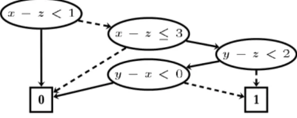
Many of the systems modeled in thentcc calculus make use of numerical constraints (see e.g., [17]). Hence, we use Difference Decision Diagrams (DDD) [15], a suitable extension of Binary Decision Diagrams (BDD) [4] to represent difference constraint expressions built from the syntax below:
φ ::= f alse| true | x − y < c | x − y ≤ c | ¬φ | φ1∧ φ2 | φ1∨ φ2 | φ1 −→ φ2 | φ1←→ φ2| ∃x.φ| ∀x.φ
A DDD can be seen as a directed acyclic graph where the set of vertex contains the terminals 0 and 1 and the non-terminals are φ formulas. The set of edges is given by the so-called high and low edges, (v, high(v)), (v, low(v)), for each non-terminal vertex. These edges represent the path taken by the DDD in case that the constraint in the vertexv holds or not. As an example, the Figure8 shows the DDD corresponding to the expressionφ = 1≤ x − z ≤ 3 ∧ (y − z ≥ 2 ∨ y − x ≥ 0). DDDs share a large number of features with BDDs. As BDDs, DDDs need to be ordered and reduced, but in the case of DDDs, it is more difficult to obtain a
canonical representation of the boolean formula. To deal with this problem, in [15] the authors propose the use of path reduced DDDs, with the aim to obtain a semi-canonical data structure, thus reducing the complexity of handling constraints. In fact, most of the operations on DDDs run in constant time.
5
Symbolic Model Checking
In Section3we saw how to build a symbolic model which is a compact representation of the behavior of a ntcc process. In Section 4 we recalled the CLTL logic able to express temporal properties of ntcc processes. The last step is to use standard techniques from symbolic model checking to verify if a process satisfies a given property. This is done by combining the model of the system and the formula to be proved. In the following we give the relevant details to perform this step.
Recall from Section 4 that the satisfiability problem of CLTL can be reduced to the same problem in LTL. Moreover, as it was shown in [5], the model checking problem for LTL can be solved by reducing it to the symbolic model checking problem for Computation Tree Logic (CTL) [9] with fairness constraints. Then, we can use all the machinery and tools developed for CTL model checking to verify programs written inntcc.
In CTL, unlike LTL, the temporal operator must be preceded by a path quantifier. Such quantifiers define where the temporal formulas must hold in the computation tree: the quantifier A, stands for “every path”, and E stands for “there exists a path”. The temporal operators to build CTL formulas are: ◦G, which means thatG holds at the next time; and GUH, which means that G holds until H holds. We recall that 3F can be defined as trueUF and 2F as ¬3¬F . Hence, in the following, we shall only use the temporal constructs “◦” and “U”. The algorithm. Given a processP and a CLTL property φ, we proceed as follows: 1. Obtain the DDD representationM for the model of the process P .
2. Compute the DDD representation T of the tableau for the (negated) formula ψ =¬(φ ∧ 2¬false).·
3. Build the set F with all the fairness constraints, i.e., all the subformulas in ψ containing the U operator.
4. Obtain the productP (through DDD operations) between the model M and the tableau ofT .
5. Apply the CTL symbolic model checking algorithm with fairness constraintsF over the symbolic productP and the property Etrue.
6. If the algorithm returns an empty set of states (satisfying the negated property), then P satisfies φ; otherwise, the algorithm returns the set of states satisfying the formulaψ as counterexamples.
Let us elaborate on the above steps. First we build the symbolic model of P as explained in Section3. Then, as shown in [5], the states σ, σ0. . . in the tableau T correspond topow(el (ψ)) where el (ψ) (the set of elementary formulas of ψ) is:
• el (F ) = F ifF is an atomic formula. • el (¬F ) = el(F ).
• el (F ∨ G) = el(F ) ∪ el(G).
• el (◦F ) = ◦F ∪ el(F ).
• el(F UG) =◦(F UG)∪el(F )∪el(G).
The transition relationT relies on the definition of the function sat(·) that maps subformulas into sets of states:
• sat (G) ={σ | G ∈ σ} if G ∈ el(ψ). • sat (¬F ) = {σ | σ 6∈ sat(F )}.
• sat (F ∨ G) = sat(F ) ∪ sat(G). • sat (F UG) = sat (G) ∪ sat(F ) ∩
sat (◦(F UG)).
Since we are dealing with formulas in LTL, the transition relation ofT satisfies the following condition for any stateσ: σ∈ sat(◦F ) iff σ0 ∈ sat(F ) for all successor σ0 of σ.
The set F of fairness constraints corresponds simply to the set of subformulas of the shape F UG in ψ. The set of fairness constraints is needed for the model checking algorithm to guarantee that in any pathπ where the formula F UG holds, it must be the case that G eventually holds. This situation can be also explained from the point of view of processes. Consider the processP = ?tell(fail) and the formula φ = 2¬fail. We know that the model of P contains a loop where fail· does not hold (due to the loop true ; true in the LTS). Then, without fairness constraints, we would be able to prove thatP satisfies φ, which is wrong.
The product P is simply obtained by operations on DDD (see, e.g., [3]). This product corresponds to the model where the negation of φ (i.e., ψ) holds and also the model of the program. Then, by running the symbolic model checking algorithm with fairness constraints [4,19] on the formula Etrue, if the resulting set of paths is empty,P satisfies the property φ, otherwise, we can exhibit a counterexample.
6
Concluding Remarks
In this paper we introduced a symbolic model to capture the behavior of ntcc pro-cesses. We showed that the internal and the observable transition relations inntcc can be neatly captured as temporal formulas. Such a compact representation was shown to be adequate to use standard techniques in model checking to automatically verify concurrent systems programmed inntcc.
We implemented a tool in Ocaml (http://ocaml.org) to execute our verifica-tion process automatically. The power of funcverifica-tional programming, the compilaverifica-tion process and the type system of Ocaml, made possible to quickly develop such pro-totype. Moreover, we provide to users a more friendly way for writing programs in ntcc by parsing their syntax with ocamllex and menhir.
The tool receives as input the ntcc program and recursively computes its symbolic representation. In order to carry out the verification, the tool com-piles the symbolic model into the format of the model checker NuSMV (http:
//nusmv.fbk.eu/NuSMV/). Then, system properties can be verified on NuSMV.
Moreover, the tool generates a PDF file with the LTS of the system as those shown in Section3’ figures.
We do not describe the implementation of our tool in depth here in order to give a higher priority to the technical aspects of our approach. The reader can find the details of the implementation as well as the execution of the examples described in this paper athttp://www.labri.fr/perso/jarias/symbolicMC.
Related work. The ideas of this paper stem mainly from the works in [16] and [22]. In [16] it was shown that the ntcc constructs ! and ? have a strong relation with the LTL temporal operators2 and 3. Moreover, the duality of these operators as greatest and least fixpoints was studied to give a denotational semantics forntcc processes based on closure operators. In [22] the author showed that the strongest postcondition of a process, notation(P ), can be characterized as a B¨uchi automata. Roughly the set(P ) contains all the possible outputs of P regardless the input. This fact was used in [22] to show that the verification problem for ntcc is decidable. We used this fact here to prove the Theorem 3.6. The construction of the B¨uchi automata in [22], however, has a non-elementary space complexity (i.e., the space complexity is worse than exponential). The construction we propose here is symbolic thus ameliorating this situation: the states do not need to be explicitly enumerated and, using logical rules, some states can be reduced in early stages of the model construction.
Automatic verification techniques for languages based on the ccp model have been also studied in [1,2,12]. In those works, the target language istccp [8]. Unlike ntcc, tccp does not consider constructs for asynchronous behavior (?P in ntcc). Moreover, the notion of time is identified with the time needed to ask and tell information to the store and the information in the store is carried through the time-units. Note that inntcc the output in a time-unit is not related to the output in the previous time-unit. For this reason, the SOS ofntcc requires both an internal and an observable transition relation and thus, the above techniques fortccp cannot be used for the verification of ntcc programs.
Finally, we refer to the work in [18] where the authors use a symbolic rep-resentation based on LTL formulas to give meaning to temporal ccp processes. Such representation was proved useful to give meaning to processes engaging in divergent computations due to universally quantified asks (not present inntcc).
Future work. Symbolic techniques in model checking aim at reducing the space and time needed to verify a given property, thus allowing for dealing with more complex systems [4,19]. However, the state explosion problem is unavoidable. In fact, the model checking algorithm for LTL is linear in the size of the model but exponential in the size of the formula to be verified. To mitigate this situation, we plan to provide tools for abstract debugging that allow the programmer to quickly find problems in her design before attempting the verification of more precise desirable properties. For that, we may rely on the abstract interpretation frameworks for the analysis of ccp programs that have been proposed in the literature (see e.g., [1,7,11,23]). Our idea is to use an abstraction of the constraint system in the lines of [11] in order to reduce the number of states generated by our technique.
Acknowledgments. We thank the anonymous reviewers for their detailed com-ments. The work of Arias has been supported by the ANR project OSSIA (ANR-12-CORD-0024).
References
[1] Mar´ıa Alpuente, Mar´ıa del Mar Gallardo, Ernesto Pimentel, and Alicia Villanueva. An abstract analysis framework for synchronous concurrent languages based on source-to-source transformation. Electr. Notes Theor. Comput. Sci., 206:3–21, 2008.
[2] Mar´ıa Alpuente, Moreno Falaschi, and Alicia Villanueva. A symbolic model checker for tccp programs. In Nicolas Guelfi, editor, RISE, volume 3475 of Lecture Notes in Computer Science, pages 45–56. Springer, 2004.
[3] Randal E Bryant. Graph-based algorithms for boolean function manipulation. Computers, IEEE Transactions on, 100(8):677–691, 1986.
[4] Jerry R. Burch, Edmund M. Clarke, Kenneth L. McMillan, David L. Dill, and L. J. Hwang. Symbolic model checking: 1020states and beyond. Inf. Comput., 98(2):142–170, 1992.
[5] Edmund M. Clarke, Orna Grumberg, and Kiyoharu Hamaguchi. Another look at ltl model checking. Formal Methods in System Design, 10(1):47–71, 1997.
[6] Edmund M. Clarke, Orna Grumberg, and David E. Long. Model checking and abstraction. ACM Trans. Program. Lang. Syst., 16(5):1512–1542, 1994.
[7] Marco Comini, Laura Titolo, and Alicia Villanueva. Abstract diagnosis for timed concurrent constraint programs. TPLP, 11(4-5):487–502, 2011.
[8] Frank S. de Boer, Maurizio Gabbrielli, and Maria Chiara Meo. A timed concurrent constraint language. Inf. Comput., 161(1):45–83, 2000.
[9] E Allen Emerson and Joseph Y Halpern. Decision procedures and expressiveness in the temporal logic of branching time. Journal of computer and system sciences, 30(1):1–24, 1985.
[10] Fran¸cois Fages, Paul Ruet, and Sylvain Soliman. Linear concurrent constraint programming: Operational and phase semantics. Inf. Comput., 165(1):14–41, 2001.
[11] Moreno Falaschi, Carlos Olarte, and Catuscia Palamidessi. Abstract interpretation of temporal concurrent constraint programs. TPLP, Published online on 10 February 2014.
[12] Moreno Falaschi and Alicia Villanueva. Automatic verification of timed concurrent constraint programs. TPLP, 6(3):265–300, 2006.
[13] Gerhard Gentzen. Investigations into logical deductions. In M. E. Szabo, editor, The Collected Papers of Gerhard Gentzen, pages 68–131. North-Holland, Amsterdam, 1969.
[14] Z. Manna and A. Pnueli. The Temporal Logic of Reactive and Concurrent Systems: Specification. Springer-Verlag, 1991.
[15] Jesper B. Møller, Jakob Lichtenberg, Henrik Reif Andersen, and Henrik Hulgaard. Difference decision diagrams. In J¨org Flum and Mario Rodr´ıguez-Artalejo, editors, CSL, volume 1683 of Lecture Notes in Computer Science, pages 111–125. Springer, 1999.
[16] Mogens Nielsen, Catuscia Palamidessi, and Frank D. Valencia. Temporal concurrent constraint programming: Denotation, logic and applications. Nord. J. Comput., 9(1):145–188, 2002.
[17] Carlos Olarte, Camilo Rueda, and Frank D. Valencia. Models and emerging trends of concurrent constraint programming. Constraints, 18(4):535–578, 2013.
[18] Carlos Olarte and Frank D. Valencia. Universal concurrent constraint programing: symbolic semantics and applications to security. In Roger L. Wainwright and Hisham Haddad, editors, SAC, pages 145–150. ACM, 2008.
[19] Kristin Y. Rozier. Linear temporal logic symbolic model checking. Computer Science Review, 5(2):163– 203, 2011.
[20] Vijay A. Saraswat and Martin C. Rinard. Concurrent constraint programming. In Frances E. Allen, editor, POPL, pages 232–245. ACM Press, 1990.
[21] Vijay A. Saraswat, Martin C. Rinard, and Prakash Panangaden. Semantic foundations of concurrent constraint programming. In David S. Wise, editor, POPL, pages 333–352. ACM Press, 1991.
[22] Frank D. Valencia. Decidability of infinite-state timed ccp processes and first-order ltl. Theor. Comput. Sci., 330(3):577–607, 2005.
[23] Enea Zaffanella, Roberto Giacobazzi, and Giorgio Levi. Abstracting synchronization in concurrent constraint programming. J. of Functional and Logic Programming, 1997(6), 1997.