Computational Amide I Spectroscopy from the ground up : building and benchmarking new tools to study disordered peptide ensembles

(1)

Computational Amide I Spectroscopy from the Ground Up:

Building and Benchmarking New Tools to Study Disordered Peptide Ensembles by

Michael Earl Reppert

B.S. Kansas State University (2009) Submitted to the Department of Chemistry

in Partial Fulfillment of the Requirements for the Degree of Doctor of Philosophy

in Physical Chemistry at the

MASSACHUSETTS INSTITUTE OF TECHNOLOGY June 2016

Signature of Author...Signature

redacted...

I5epartment of Chemistry April lIt, 2016

Signature redacted

C e r t i f i e d b y ... ... . . . . --- -m- ----..-- V ;nd i Tokmakoff Professor of Chemistry

Accepted by...Signature

redacted

Robert W. Field Chairman, Departmental Committee on Graduate Students MWASSACHUS-EflS INSTITUTE

OF TECHNOLOGY

JUN 2 3 2016

LIBRARIES

Signature redacted

Professor Moungi G. Bawendi

Signature redacted

Professor Andrei Tokmakoff Thesis Supervgir

(4)

(5)

Computational Amide I Spectroscopy from the Ground Up: Building

and Benchmarking New Tools to Study Disordered Peptide Ensembles

by

Michael Earl Reppert

Submitted to the Department of Chemistry on April 12th 2016 in Partial Fulfillment of the

Requirements for the Degree of Doctor of Philosophy in Physical Chemistry

ABSTRACT

In the "form follows function" paradigm of structural biology, we seek to understand-and control-protein function based on our knowledge of protein structure. This process is often difficult for intrinsically disordered proteins and peptides (IDPs) which possess inherent structural disorder in their functional forms. A prototypical example is elastin, a disordered structural protein that provides elastic properties to skin, lungs, and other connective tissues. In such cases, the "form" of the protein must be thought of not as an individual structure, but as a heterogeneous ensemble of structures. The characterization of such ensembles is complicated both by the inherent disorder of the system and by the fact that many common experimental techniques function poorly when applied to IDPs. In this work, we present our recent progress in developing experimental and computational tools for characterizing IDP ensembles using Amide I (backbone carbonyl stretch) vibrational spectroscopy. In this approach, the infrared (IR) absorption frequencies of isotope-labeled amide bonds act as sensitive probes of local electrostatic environment and, ultimately, of local structure. By producing and characterizing experimentally a progression of increasingly complex model systems ranging from dipeptide fragments to isotope-labeled proteins, we develop an efficient and robust spectroscopic model capable of predicting Amide I vibrational frequencies from atomistic protein structures to within a few cm-1 of error. We apply these methods to the analysis a family of short (eight-residue) elastin-like peptides (ELPs), fragments of the elastin protein, whose local structure is believed to be critical to elastin function. Using our empirically-parameterized frequency maps, we test and refine molecular dynamics ensembles by quantitative comparison against isotope-labeled experimental data. This combination of isotope-labeled IR data, high level spectroscopic modeling, and well-sampled molecular dynamics ensembles provides both local conformational insight into the molecular structures underlying elastic function and a point of departure for testing and refining force-field based structure prediction methods for intrinsically disordered systems.

Thesis Supervisor: Andrei Tokmakoff Title: Professor

(6)

(7)

Then I applied myself to the understanding of wisdom,

(8)

(9)

Acknowledgements

In the writing of this text, I owe deep debts of gratitude to many people.

To my advisor Andrei Tokmakoff for his support and encouragement and for letting me try crazy ideas in the lab. To my friend and labmate, Luigi De Marco, for friendship, support, honest opinions, grilled meat, and late nights at the lab hacking away (unsuccessfully) at the BCH formula. To Anish Roy for his hard work in many of the projects described here. To the Pauls (Stevenson and Sanstead) for experimental backup and fun with an unending supply of practical jokes. To Kevin Jones for his example of serious scientific practice and academic integrity, all with a sense of humor ("They make these toasters...").

To Ryszard Jankowiak, Virginia Naibo, Nhan Dang, and Tonu Reinot for giving me a start in research and for imbuing me with a love of academic work. To Chi-Jui Feng and Rajib Biswas for assistance and commiseration in computational matters, for good food, and for good card games. To Jeremy Tempkin for brainstorming sessions and computational assistance. To Pete Dahlberg for sharing a love of science, a box of good tea, and early morning chats in the office when nobody else was around and I really didn't want to be working anyway. To John Phillips for outstanding facility support and a few solid nuggets of life advice along the way.

To my father for teaching me that the world is a fascinating place and that very little exists that isn't worth exploring. To my mother for teaching me to laugh while I learn. To my sisters for pushing me to do my best and for being ready to talk when things didn't go right. To my brother Isaac for recognizing obscure movie references, snorkeling with me in fresh snowmelt, and always being ready to talk about life. To Melaku Zewde, Daniel Szatkowski, Joel Cohen, Adam Hannon, Ben Lynerd, and John Kimbrough for support, encouragement, and a challenge toward a life of integrity, faith, and personal growth throughout the PhD process. To Peter and Kathryn Scherpelz, Jessica Gonzalez, Alex Ling, Ben Sheppard, and Jasmine Tan for fun, fellowship, and the confidence of knowing that you had my back. To my wife Deborah for sticking with me when things are hard. And, above all, to my God for his gift of love, life, science, and a reason to keep going.

(10)

Funding

I would like to thank the National Science Foundation for a Graduate Research Fellowship and for funding from Grant Nos. CHE-1212557 and CHE-1414486. Both sources of funding were instrumental to the research described here.

(11)

List of Figures

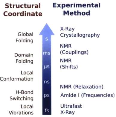
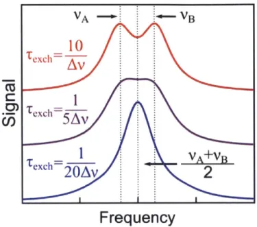
Figure 1.1. Overview of functional roles carried out by intrinsically disordered proteins. A dapted w ith perm ission from Ref. 5 ... 27 Figure 1.2. Stability time scales in biophysical structure and measurement. The column on the left provides a rough guideline for the stability time scale of various structural features. The column to the right provides for comparison a schematic outline of the time scales required for various methods to determine distinct signals for distinct structures. ... 28 Figure 1.3. Coalescence of two absorption peaks for two exchanging species A and B. As the exchange time between the two structures decreases relative to the (inverse of the) frequency splitting, the two peaks coalesce to give rise to a single feature at the average frequency 'A + VB

2 ... 30

Figure 1.4. Sensitivity of the Amide I vibrational frequency to local electrostatic interactions. Upper panel: As hydrogen bond contacts are formed and strengthened, the amide C=O bond weakens and the vibrational potential for the Amide I mode broadens, lowering the frequency of the corresponding vibration. Lower panel: This electrostatic sensitivity is enhanced by the two active resonance structures of the amide bond. Hydrogen-bonding interactions shift the resonance equilibrium toward a charged structure in which the C and 0 atoms are linked by only a single bond... 32 Figure 1.5. Amide I vibrational absorption spectra for the L-Leu-D-Leu dipeptide in pure D20, a 50:50 (by volume) mixture of D20 and deuterated methanol (MeOD), and pure MeOD. 33 Figure 1.6. Unlabeled Amide I 2DIR spectra for poly-L-lysine (frame A, n-sheet conformation) and myoglobin (frame B, dominantly helical structure)... 34 Figure 1.7. Representative collapsed and extended structures for the PG-turn region in XPGVG peptides. The collapsed structure takes the form of a partially-frayed

P-turn.

... 37 Figure 2.1. Mnemonic diagrams for expanding the third-order response function... 80 Figure 2.2. Ladder diagrams for the third-order response tensor, showing interaction matrix elem ents. ... 8 1 Figure 2.3. Arrow/Ladder diagrams for third-order response functions... 84

(16)

Figure 2.4. Comparison of rephasing and nonrephasing signals for a two-level system. A phenomenological damping term with F / c =10 cm- is included to give the peaks finite width. Red color indicates positive contours, while blue indicates negative... 92 Figure 2.5. Sum and difference 2D spectra for a two-level system. Parameters are the same as in F igu re 2.4... 93 Figure 4.1. Schematic outline of the roles of gamide and gspec in simulating Amide I vibrational spectra. First, gamide converts the MD structural trajectory into a parameter trajectory of Hamiltonian and transition dipole moment matrix elements. Next, gspec converts this parameter trajectory into a simulated spectrum... 154 Figure 4.2. Example mdp file contents for an unconstrained energy minimization run. ... 189 Figure 4.3. System potential energy as a function of time during a typical energy minimization run. Note that by the end of the simulation, the energy is no longer decreasing rapidly, indicating the end of the equilibration period... 192 Figure 4.4. Contents of an example mdp file nvt .mdp used here for equilibration of the solvent box ... 194 Figure 4.5. Example submit script using the SLURM scheduler. The introductory lines beginning with "#" are scheduler instructions, while the remaining text indicates the commands that are actually to be performed when the script executes. ... 196 Figure 4.6. Temperature trajectory from a typical 100 ps NVT equilibration run. Note the rapid increase in temperature during the first several ps, followed by largely stable temperature throughout the rem ainder of the simulation... 198 Figure 4.7. Example mdp file contents for a 1 ns NPT equilibration run... 199 Figure 4.8. Volume (left) and pressure (right) trajectories for a typical 1 ns NPT equilibration run...20 1

Figure 5.1. (A) Experimental FTIR absorption spectra for the GG dipeptide as a function of pH. Dashed vertical lines mark the Amide I peak maxima. See text for details. (B) Frequency histograms (4 cm' bins) for 23 standard dipeptides under acidic (yellow), neutral (red), and basic (black) conditions... 2 15 Figure 5.2. (A) Structure of a generic dipeptide; our coordinate system is defined so that the x-axis points along the amide C=O bond and the y-axis is in the plane of the amide unit. (B - E) Scatter plots of experimental peak frequencies for 23 standard dipeptides with individual

(17)

electrostatic variables evaluated from 5 ns CHARMM27 MD simulations (see labels in figure). ... 2 16 Figure 5.3. Correlation scatter plots for experimental Amide I peak frequencies (horizontal axis) and predicted frequencies (vertical axis) from linear least-squares best fit equations to various electrostatic parameters as labeled. The c values reported for each frame are Pearson correlation coefficients... 218 Figure 5.4. Scatter plots of experimental Amide I peak frequencies with MD electrostatics for CHARMM27 (left panel) and OPLS-AA (right panel) force fields. Amino acid composition is labeled by color (see legend). The inset for each panel plots an error histogram (deviation between experimental and best-fit simulation frequencies) for the 23 standard dipeptides in each data set. ... 220 Figure 5.5. Scatter plot comparing the average electric field values E for CHARMM27 and OPLS-AA trajectories. Data points are colored according to amino acid composition (see legend). The dashed line is the least-squares best fit line for the standard dipeptide data (black points): EOpa = 0.7246. EcHARM - 0.033 The correlation coefficient is 0.975... 223

Figure 5.6. A comparison of experimental absorption spectra (blue circles) with simulated frequency histograms (dashed lines) and absorption spectra (solid lines) for the VT dipeptide under neutral and basic conditions. Note that the clipped peak near 1600 cm- is due to the C-terminal carboxylate absorption peak which is not included in our simulations... 225 Figure 6.1. Excluded atom conventions for JO and SG electrostatic maps (A) and DC/DO electrostatic maps (B). Atoms displayed in blue are included in electrostatic frequency shift calculations for the amide bond displayed in red. The bond atoms themselves (red) and non-sidechain atoms of neighboring amino acids (grey) are excluded for electrostatic calculations.245

Figure 6.2. Structure of Met, Leu, Gly, Phe, Val, and Ala labeled variants of NuG2b with labeled sites highlighted in red and solvent exposed surfaces shaded in grey. Residue numbering begins with the N-terminal Met denoted as residue zero... 247 Figure 6.3. Experimental FTIR spectra for isotope labeled NuG2b. Blue curves indicate the IR absorption spectrum of the 13_{C labeled peptide and red curves indicate}

13C180 peptides. Black spectra are the unlabeled reference. Spectra are normalized to have unit area between 1525 cm' and 1700 cm -'... 24 8

(18)

NuG2b isotope-labeled peptides using different literature maps and force fields. The top panel shows the entire Amide I frequency range. The lower panel shows a closeup of the 13C'80

isotope label region... 249 Figure 6.5. Average MSD values for the four simulation methods of Figure 6.4, averaged across all isotope labels. The top panel shows the results of the main band calculation (integration range 1600-1690 cm~'), reflecting agreement in the main band region. The lower panel shows the results for the isotope label region (1525- 600 cm'i)... 251 Figure 6.6. Experimental difference spectrum (black curves) between the various labeled NuG2b peptides and the unlabeled reference spectrum. Gaussian fits (red curves) are applied to the positive-frequency portion of the difference spectrum (solid black curve). The difference spectrum reflects the increased absorption in the label spectrum due to 13CI'O labeled sites. Parameters for all Gaussian components are provided in Table 6.3. Structural assignments for major components are summarized in Table 6.4... 252 Figure 6.7. Scatter plots of simulated vs. experimental mean frequencies (left column) and FWHM (right column) for the assigned site clusters in Table 6.4 (top row). The inset number represents the RMS error between experimental and simulated values. The two data points in each plot marked with x symbols represent the Phe helix and sheet clusters. ... 256 Figure 6.8. Simulated (red) absorption spectra for isotope-labeled NuG2b peptides using the DC (left column) and DO (right column) electrostatic maps and CHARMM27 and OPLS-AA trajectories with their native charges (upper left and lower right frames) or "swapped" charges (OPLS-AA charges on a CHARMM27 trajectory or vice versa). The data in the two diagonal plots (upper left and lower right) are identical to that shown in Figure 6.4. Black curves show experim ental spectra for reference...258

Figure 7.1. Experimental (shaded curves) and simulated (black solid lines) Amide I absorption spectra for isotope-labeled NuG2b for four different electrostatic maps. The dotted lines show Gly label spectra after introducing the charge correction described in the text... 276 Figure 7.2. Calculated electric field vs. experimental peak absorption frequency for dipeptides in our standard data set. Green x's indicate dipeptides of the form NH2-Gly-Xxx-COO-. Red x's indicate the same data points after the introduction of our Gly charge correction. ... 2 7 7 Figure 7.3. Error surfaces for 4P maps against dipeptide and NuG2b datasets as a function

(19)

of the coefficients CN and CH. Left: Standard error between predicted and experimental dipeptide mean frequencies. Right: MSD between simulated and experimental spectra averaged across all N uG 2b isotope labels... 279 Figure 7.4. Comparison of experimental (shaded) and simulated (black lines) absorption spectra for NuG2b isotope labels using the optimized 4P (solid) and 3F (dashed) maps. ... 281 Figure 8.1. Experimental (black) and simulated (blue) absorption spectra for three globular proteins of varying secondary structure content: myoglobin (MGB), a primarily helical protein; NuG2b (NGB), a mixed sheet/helix fold, and

P-lactoglobulin

(BLG), a primarily

P-sheet protein.

All spectra are norm alized to unit area. ... 288 Figure 8.2. Schematic overview of the parameters required for different electrostatic coupling models. Black indicates equilibrium parameters (e.g. static charges). Blue indicates parameters describing nuclear motion. Red indicates electronic charge flux (e.g. transition charges). Orange indicates effective transition dipole parameters, e.g. effective transition charges in the ECC model and effective transition dipole parameters in the TDC model. See text for detailed descriptions of each m odel... 291

Figure 8.3. Simulated absorption spectra for Myoglobin (blue), NuG2b (green), and

P-lactoglobulin (red) under the TDC electrostatic coupling model for various transition dipole moment magnitudes (0.06 to 0.12 D2 in squared magnitude) and rotation angles relative to the C=O bond (50 to 200). Experimental spectra (black curves) are shown for comparison with each spectrum ... 294 Figure 8.4. ECC-model calculations (solid lines) for myoglobin (blue), NuG2b (green), and

p-lactoglobulin

(red). For comparison, calculations under the TDC model are shown as dashed lines. Black curves show the corresponding experimental spectra... 297 Figure 8.5. Structural definitions of adjacent amide units... 298 Figure 8.6. The variation of non-vanishing matrix element coefficients with dihedral angle. The horizontal axis corresponds to variation in the

#

dihedral angle and the vertical axis to variations in y/ . ... 300 Figure 8.7. Potential optimization scheme for complete Amide I map development. ... 301 Figure 8.8. Reference frames for Amide I coupling calculations. The unit-specific frames illustrated in the upper panel follow the usual literature convention. For describing through-bond interactions, a bond-centric frame as illustrated in the lower panel is more convenient... 308

(20)

Figure 8.9. Representative conformations of the two-bond unit with the (#, V/) dihedral angles fixed at various values... 309

Figure 8.10. Matrix elements for the 3x3 rotation matrix m(2

) presented as a function of the

dihedral angles ($, V ). ... 313 Figure 9.1. Amide I absorption spectra for the four peptides studied in this work. Foreground spectra are for peptides with a 13C 0 isotope label introduced at the XP carbonyl group ... 324 Figure 9.2. Experimental 2DIR spectra for unlabeled GP, AP, VP, and VPV peptides dissolved in D20 (pD~l, top) and TFE (bottom). Spectra are collected in the ZZYY polarization at a w aiting tim e of 150 fs... 326 Figure 9.3. Structural analysis of 400 ns OPLS-AA MD ensembles for the GP, AP, VP, and VPV peptides. The top panel shows representative structures uniformly sampled from the complete trajectory and aligned around their proline ring. The remaining panels plot representative distributions and statistics for (A) turn extension, (B) radius of gyration, (C) XP carbonyl-to-solvent hydrogen bonds, (D) XP carbonyl-to-peptide hydrogen bonds, and (E) total X P carbonyl hydrogen bonds... 329 Figure 9.4. Comparison of experimental isotope-labeled Amide I spectra against simulated spectra for the 400 ns OPLS-AA simulations reported above using the single-point field (IF) m ap and the JR m ap... 331

Figure 9.5. Simulated absorption spectra using the JR and IF maps as a function of turn extension d. Experimental spectra are shown as shaded curves for reference... 332 Figure 9.6. Maximum entropy (ME) refinement of the ELP structural ensembles for GP, AP, VP, and VPV peptides. In these calculations, the ensemble is reweighted by maximizing the cross-entropy subject to the constraint that the ensemble mean frequency match the experimental value. In the left panel, shaded curves represent experimental Amide I isotope-labeled spectra, while black lines represented spectroscopic simulations before (dashed) and after (solid) ME refinement. In the right panel, the shaded curves represent raw MD data; the darker, unshaded curves represent M E-refined statistics... 335 Figure 9.7. ME ensemble refinement using both mean and variance constraints. In the left panel, shaded curves represent experimental Amide I isotope-labeled spectra, while black lines represented spectroscopic simulations before (dashed) and after (solid) ME refinement. In the

(21)

right panel, the shaded curve represents raw MD data; the lighter, unshaded curve represents M E -refined statistics... 337 Figure 9.8. Turn-distance histograms for various peptide/force field ensembles both before (shaded curves) and after (unshaded lines) ME refinement constraining both mean and variance to match experiment. Thick solid lines represent ME-refined ensembles under the assumption of no map error, while thin dashed lines represent ME ensembles under the assumption of -5 cm' map error (long-dashed curves) or +5 cm' error (short-dashed curves). ... 338

Figure 9.9. Predicted population of extended conformations (turn distance larger than 5 A) for each peptide and force field. Raw MD predictions are plotted as round data points linked by a thick black line. ME-reweighted values are represented by vertical bars with error bars representing the maximum and minimum population obtainable within an assumed map error interval of -5 cm - to +5 cm ... ... .. ... ... ...339

(22)

(23)

List of Tables

Table 5.1. Best-fit data for various combinations of electrostatic variables evaluated for the CHARMM27 force field against experimental frequencies for our 23 standard dipeptides. The first data column presents the sample standard deviation (F) of the error between best-fit prediction and experimental values. The second column reports the predicted zero-field (i.e. vacuum) frequency, and the third column the linear coefficients for the respective variables (see, e.g. Eqs. 4 and 8). The units on the potential are E / e0 and on the field Eh / ae, , as above. Note that for the potential fits, the coefficients are constrained to sum to zero. ... 230 Table 6.1. Summary of the Amide I maps used in this study. Electrostatic site specifications refer to atomic sites of the CONH peptide linkage; "Jansen" refers to the NNFS, NNC, TCC, and transition dipole models of Ref.14; "Torii" refers to the transition dipole and TDC model of Ref.36. In specifying electrostatic components, the x axis is taken to point along the C=O bond axis, while the y axis lies in the amide plane and the z axis is perpendicular to it. ... 246 Table 6.2. Frequency shift coefficients for the JO, SG, DC, and DO electrostatic maps used for spectral simulations. All coefficients are in units of cm- per elementary electrostatic unit

(Eh/e, for potential, EhlaOe) for electric field, and E2a/2eo for field gradient, where Eh indicates

Hartrees, e0 is the elementary charge, and ao is the Bohr radius). ... 248 Table 6.3. Fit parameters for various labeled residues. For each component, the relative area (between 0 and 1), mean frequency, and full width at half maximum are reported... 255

Table 6.4. Fit parameters for various site group assignments. The Leu, Val, and Phe parameters describe individual Gaussian components found to be assignable to individual clusters of sites. The parameters for the Gly and Ala sites are calculated from the total Gaussian fit (the sum of two Gaussian components). In all cases, the reported peak width is the full width of the curve at half the m axim um value... 256 Table 7.1. Atomic partial charge assignments for the atoms CA, HAl, and HA2 in mid-chain and NH2-capped N-terminal glycine residues. Each primary entry indicates the charge

assigned by the CHARMM27 force field; numbers in parentheses indicate our corrected glycine charges used for spectroscopic calculations. All charges are in units of elementary charge e,.

Charge assignments for other protonation states of the Gly residue (NH3+ N-terminal, and COO-/COOH C-terminal) are unmodified from the force field assignments. ... 280

(24)

Table 7.2. Dipeptide standard error (udi,), NuG2b MSD, and frequency map coefficients for the dipeptide-optimal 4P map (4PN-4), NuG2b-optimal 4P map (4PN- 150), and 3F translation of the 4PN -150 m ap. ... 284 Table 9.1. Peak frequencies for experimental and simulated isotope-label peak frequencies for four ELPs, quoted in cm'. Simulations refer to OPLS-AA MD simulations using the single-point field (IF) and JR electrostatic m aps. ... 326 Table 9.2. Predicted population of extended conformations (turn distance larger than 5

A)

for each peptide and force field. ME-refined values are reported with average absolute error values (the average between absolute errors on the high and low sides) compared with raw MD populations in parentheses... 342

(25)

"It is the pervading law of all things organic and inorganic, of all things physical and metaphysical, of all things human and all things superhuman, of all true manifestations of the

head, of the heart, of the soul, that the life is recognizable in its expression, that form ever follows function. This is the law."- Louis Sullivan

Chapter 1: Introduction

Intrinsically Disordered Proteins

Proteins are the molecular workhorses of living systems. While nucleic acids encode genetic information, and carbohydrates and lipids store energy and form molecular structures, proteins are the movers and shakers that organize, assemble, move, distribute, and modify these molecular components into functional entities. Proteins are responsible for mechanical processes such as muscle motion, chemical processes such as digestion and metabolism, and structural processes such as cellular division and reproduction.

The central role of proteins in biological function has prompted decades of intense research focused on determining the specific physical and chemical mechanisms that enable proteins to accomplish such a wide range of tasks. With the advent of protein crystallography in the mid-1900s, it became apparent that many functional proteins adopt highly specific three-dimensional structures, precisely tuned to their specific tasks. The later development of nuclear magnetic resonance (NMR) experiments greatly expanded the range of proteins accessible to structural analysis. A key advantage of NMR experiments is that they can be conducted on proteins in solution rather than in the delicate protein crystals required for X-ray crystallography. An additional advantage is that NMR spectroscopy allows access to dynamical protein processes, such as structural changes and rearrangements. Armed with these tools, researchers have determined the structures of thousands of functional proteins, enabling in many cases a detailed analysis of protein structure and function.

Building on this wealth of structural data, the classic "form follows function" paradigm of structural biology for many years operated under an implicit assumption that specific

(26)

mechanistic tasks require specific, stable protein structures. Recent evidence, however, has revealed a large and growing class of functional proteins that lack a well-defined native structure either for part or all of their sequence."2 _{At current count, it is estimated that 44% of} protein-coding genes in the human genome contain intrinsically disordered regions of at least 30 amino

3,4

acids in length.3, These intrinsically disordered peptides and proteins (IDPs) accomplish an astonishing array of specific molecular tasks despite their intrinsic lack of structural stability (see Figure 1.1).3,5 For example, a number of IDPs have been identified to function in cellular signaling processes, where their lack of a single native structure allows them to bind to multiple signaling partners.6 Others function as nucleation points for larger complexes, using their structural flexibility to recruit multiple binding partners and link them together.3 _{In protein and}

RNA chaperones, intrinsically disordered regions (IDRs) within the larger folded protein appear to play important functional roles in binding and refolding other proteins.''8 _{Although in many} cases intrinsic disorder is present largely in a pre-functional state (e.g. signaling proteins that undergo coupled folding and binding processes ), for some proteins, disorder appears to play an essential functional role. A prototypical example is the mammalian structural protein elastin that lends elasticity to skin, lungs, and other connective tissues.'0 Although the molecular mechanisms of the process are not understood in detail, the presence of extreme structural heterogeneity-that is, the availability of a large number of energetically similar structures at many different total protein extension lengths-appears to play a central role in the function of

the system as an "entropic chain." 1),11

In light of these findings, the functional "form" of an intrinsically disordered system must be thought of not as a single structure but as a conformational ensemble of structures, each of which is thermally accessible under physiological conditions. In the context of IDPs, then, the problem of the structural biologist is not to determine a single structure-or even a small number of structural variants-but to directly characterize the conformational ensemble, assessing the structure, population, and functional significance of tens, hundreds, or even thousands of distinct conformations. Two central challenges make such IDP ensemble studies extremely difficult.

(27)

IDPs

entropic chains reCO"nlitionl

directl% function

due to disorder as spring, hritle, linker

transient binding permanent

display sites Chaperones effectors -ISSCIIIb)LT

site% of post- . modulate the a4%Nehmhle

translational the fold g aCtiMil ol a Complexes or

modification of RNA or protein partner mioleculc target acti' it-,

tbinding

Is Is CA VenWIris

store andlor

neutraliit

%mall ligands%

Figure 1.1. Overview of functional roles carried out by intrinsically disordered proteins. Adapted with permission from Ref. '

I First, the sheer number of distinct structures-and hence often overlapping signals in

experimental measurements-severely complicates the interpretation of experimental data. Even computational studies in which individual structures are trivially separable struggle both to adequately sample relevant configurations and to assign physically meaningful structural classifications. The practical effect of such complexity is that IDP structural ensembles must usually be described only in terms of reduced-dimensionality or ensemble-averaged quantities such as hydrodynamic radius, bulk secondary structure content, or end-to-end distance.

Second, IDP structural analysis is complicated on a more technical level by the fact that many standard structural tools suffer from signal suppression or distortion when applied to IDP ensembles. Although the origin and severity of such complications vary by technique, most are ultimately a result of the increased rate of structural fluctuations in IDPs relative to more stably

-folded proteins (see Figure 1.2). Traditional X-ray crystallography can be thought of as an extreme example of such complications, since intrinsic structural disorder precludes the preparation of crystals required for scattering measurements. For most other techniques, the situation is more complicated. Low-resolution structural tools such as label-free infrared (IR) and

(28)

circular dichroism (CD) spectroscopies offer insight into total secondary structure content, but

provide little site-specific information. Label-pairing methods like Frster resonance energy

transfer (FRET) and electron paramagnetic resonance (EPR) spectroscopies provide excellent

long-range distance sensitivity, although again at a coarse-grained level.13J4

Structural

Coordinate

Global Folding Domain Folding Local Conformation H-Bond Switching Local Vibrations

Experimental

Method

X-Ray Crystallography NMR (Couplings) NMR (Shifts) NMR (Relaxation) Amide I (Frequencies) Ultrafast X-Ray

Figure 1.2. Stability time scales in biophysical structure and measurement. The column on the left provides a rough guideline for the stability time scale of various structural features. The column to the right provides for comparison a schematic outline of the time scales required for various methods to determine distinct signals for distinct structures.

NMR spectroscopy provides by far the most holistic picture available of IDP structural ensembles. But even here the interpretation of measured NMR signals is complicated by a conflict between the intrinsic measurement time scale of the NMR experiment and the conformational exchange time scale of IDP structures. 5 While the large-scale structural rearrangements typically of interest in stably-folded proteins (e.g. global folding and domain rearrangement) occur generally over a time scale of milliseconds to seconds (see Figure 1.2), the

(29)

local conformational fluctuations so abundant in disordered systems occur on the much shorter scale of nanoseconds to microseconds.16-18 These rapid exchange events complicate many NMR-based measurements due to an effect called motional narrowing in which rapidly exchanging structures give rise not to a large number of individual spectroscopic signals but to a single, narrow-band signal reflecting the average properties of the system. A classic example of such effects is the coalescence of two NMR peaks into a single peak under rapid structural exchange as illustrated schematically in Figure 1.3. A useful (and quite general) rule of thumb is that spectroscopic features merge to become indistinguishable from one another when the exchange time between the chemical species of interest is shorter than the intrinsic coalescence time

1 - 1(1)

Av _|VA _VB

where VA and VA are the oscillation frequencies of the signals from two distinct but

exchangeable species A and B. For 1C NMR measurements, Larmor precession frequencies typically span a range on the order of tens of MHz, corresponding to a typical coalescence time on the order of a microsecond.'15' 9 As a result, although NMR undoubtedly remains the most comprehensive tool available for IDP structural analysis, sub-microsecond conformational exchange processes often limit the ability of NMR-based methods to directly probe the full distribution of structures present in a disordered ensemble.

Given these challenges, interest has increased in recent years in the development of novel techniques whose intrinsic measurement time scale is fast relative to the time scale of IDP structural fluctuations. The present work explores the utility of one such method, isotope-enriched Amide I vibrational spectroscopy for IDP ensemble characterization. Although this work makes extensive use of experimental spectroscopic data, computational work plays the essential role of relating measured experimental data to specific atomistic structures. In the remainder of this chapter, we first provide a general introduction to Amide I vibrational spectroscopy and then describe the specific disordered system of interest to our group: a family of short, elastin-like peptides whose propensity for intrinsic disorder appears to mimic (and likely to facilitate) the elastic function of the physiological elastin protein.

(30)

VA -B

Frequency

Figure 1.3. Coalescence of two absorption peaks for two exchanging species A and

B. As the exchange time between the two structures decreases relative to the

(inverse of the) frequency splitting, the two peaks coalesce to give rise to a single

V V

feature at the average frequency

A

B.

2

Amide I Spectroscopy

Amide I vibrational spectroscopy has long been known as a robust experimental probe of

protein secondary structure content in solution.2 0 The amide vibrational mode consists primarily

of the stretching vibration of backbone amide carbonyl groups, with a smaller contribution from the backbone C--N stretch and N-H or N-D wagging motions. Amide I vibrations absorb in the

1600 - 1700 cm-' range, and experiments are typically carried out in deuterated water (D₂0) to

avoid overlap with the H20 bend absorption band near 1640 cm'. The structural sensitivity of

Amide I spectroscopy stems from the delocalization of Amide I vibrational modes over many sites across the protein backbone. The energetic structure of the resulting exciton-like states is

acutely sensitive to the spatial arrangement of the amide oscillators.2' As a result, different

secondary structure elements (o-helix, 3-sheet) give rise to distinctive Amide I line shapes in experimental spectra. Helical structures give rise to a single, largely featureless absorption band

(31)

intensities.20 _{The lower frequency peak occurs near 1620-1630 cm-1 and corresponds to a}

vibrational mode in which all oscillators vibrate in phase with one another, producing a net dipole perpendicular to the alignment of the sheets. The higher frequency peak occurs with much lower intensity near 1680-1690 cm-1 with a net dipole parallel to the sheet alignment.2 2 Disordered and random coil structures typically absorb near 1640 cm', often overlapping with helical structures, but showing a broader line width. These canonical spectroscopic assignments have been known for many years and provide a robust means of quantitatively assigning bulk secondary structure content for proteins in solution.20

More recently, Amide I spectroscopy has been developed as a probe of local protein

structure through the use of site-specific isotope labeling.2 3

-26 _{In this approach,}13_{C or}₁₈₀_isotope

labels are introduced into specific amide groups along the protein backbone. The resulting increase in the reduced mass of the carbonyl oscillator induces a frequency shift of either 40 cm-1

(13C) or 60 cm- (1 3C=180), decoupling the labeled amide site from its neighbors and allowing its

spectroscopic features to be measured independently.2 3 _{The structural utility of this approach} stems from the acute sensitivity of Amide I vibrational frequencies to their local electrostatic environment, particularly to hydrogen bonding interactions. As illustrated in Figure 1.4, local electrostatic interactions can either stiffen or weaken the Amide I vibrational potential, shifting vibrational frequencies in response to local structural changes. Hydrogen bond donation to the carbonyl oxygen in particular stabilizes the alternate enol-like resonance structure, giving rise to an increased negative charge on the 0 atom, a significantly weakened C=O bond, and a corresponding red-shift of-16 cm-1 to the Amide I transition frequency.2 7

(32)

I,

C _CO

>=O-

--....D-N C==0 .-- D-N\

>-N

D-C

Increasing H-bond strength

C=O C_ -~

D-N( D-N+

Figure 1.4. Sensitivity of the Amide I vibrational frequency to local electrostatic interactions. Upper panel: As hydrogen bond contacts are formed and strengthened, the amide C=O bond weakens and the vibrational potential for the Amide I mode broadens, lowering the frequency of the corresponding vibration. Lower panel: This electrostatic sensitivity is enhanced by the two active resonance structures of the amide bond. Hydrogen-bonding interactions shift the resonance equilibrium toward a charged structure in which the C and 0 atoms are linked by only a single bond.

A simple example of this hydrogen-bonding sensitivity is presented in Figure 1.5. Fourier

transform infrared (FTIR) absorption spectra for the NH3+-L-Leucine-D-Leucine-COO dipeptide

are presented in D20, deuterated methanol (MeOD), and a 50/50 mix of the two solvents. In

D20, the dipeptide's single amide bond absorbs near 1651 cm- , with a distinct, asymmetric tail

trailing off toward higher frequency. On the addition of 50% MeOD, this high-frequency tail

grows into a distinct peak near 1666 cm, a 15 cm'1 blue shift compared to the D20 spectrum.

The frequency shift is due to the switch from an aqueous solvation environment capable of

donating two hydrogen bonds to the amide carbonyl group, to the much weaker solvation environment of the water/ methanol mixture in which the peptide accepts only a single hydrogen

(33)

bond. In pure MeOD, this trend is accentuated by the appearance of an entirely new peak near 1684 cm-1, a further blue shift of 18 cm , evidently corresponding to a subpopulation of amide groups which are unable to form any hydrogen bonds to the solvent.

C

D2

D

2

0/MeOD

MeOD

1625

1675

Frequency (cm-

1 ₎

Figure 1.5. Anide I vibrational absorption spectra for the L-Leu-D-Leu dipeptide

in pure D-), a 50:50 (by volume) mixture of D-0 and deuterated methanol

(MeOD), and pure MeOD.

Nonlinear methods such as two-dimensional infrared (2DIR) spectroscopy expand the capabilities of linear absorption measurements by spreading measured signals across multiple

frequency axes and by increasing the sensitivity of the method to structural dynamics.28 In

contrast to conventional absorption measurements, 2DIR experiments employ an ultrafast laser system to excite the protein sample with a series of laser pulses separated by carefully controlled time delays. By varying the time delay between the laser pulses and Fourier-transforming the signal, one obtains a two-dimensional correlation plot of vibrational frequencies at two different points in time, separated by anywhere from 0 fs to a few ps. Intuitively, one can think of the two

(34)

variable time delay T2 . In 2DIR spectra, positive diagonal peaks are always accompanied by

negative features at lower frequency (approximately 16 cm' for Amide I) in (0 corresponding

to excited state absorption. This characteristic doublet shape is a result of the anharmonic nature of the Amide I vibration and is ubiquitous in 2DIR spectra.

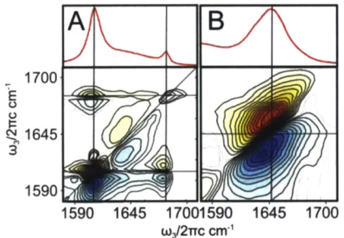
For bulk protein spectra, this two-dimensional plot aids in structural sensitivity by lowering spectral congestion and giving rise to distinctive cross-peak patterns for different secondary structure elements. As an example. Figure 1.6 shows Amide I FTIR and 2DIR spectra for poly-L-lysine in its f-sheet form (Frame A) along with the spectrum of Myoglobin, a predominantly helical protein (Frame B). The upper panels plot FTIR absorption spectra, showing the distinctive P-sheet peaks near 1620 and 1680 cm' for poly-L-Lysine, and an a-helix peak near 1645 cm' for Myoglobin. The 2DIR spectra in the lower panels show similar features along the diagonal. Off the diagonal, a distinctive cross-peak pattern is apparent in the

p-sheet

spectrum, with a clear cross-peak forming between the 1620 and 1680 cm' features. This distinctive P-sheet cross peak (often appearing in more complex systems as a long ridge rather than a separate peak) provides a useful metric for measuring

p-sheet

secondary structure content in solvated proteins.29 Even in disordered (e.g. thermally denatured) systems, residual

P-sheet

content often makes itself known through similar features in 2DIR spectra.3 0

A

B

/\

1700 E 1645 1590 1590 1645 17001590 1645 1700 w3/2rrc cm-'

Figure 1.6. Unlabeled Amide I 2DIR spectra for poly-L-lysine (frame A, f-sheet conformation) and myoglobin (frame B, dominantly helical structure).

(35)

In isotope-labeled experiments, the variable time-delay r, available in 2DIR spectra provides access to local solvation dynamics of the isotope-labeled sites. At short time delays

(, ~0), the 2DIR spectrum provides a two-dimensional snapshot of instantaneous frequency heterogenity. Elongation along the diagonal in 2DIR spectra is a hallmark of inhomogenous broadening, a result of independent absorption events by amide groups in many different local environments. If these different environments are stable on the picosecond time scale, the spectrum will change little as the time delay r, is scanned. On the other hand, if local structural fluctuations take place during the time delay between laser pulses, the initially elongated Amide I spectrum becomes round and homogenous as the local environment of each amide group

evolves in time.28

In the context of IDP ensemble analysis, Amide I spectroscopy is particularly attractive due to its ultrafast intrinsic time scale. Thanks to the much higher intrinsic frequency of vibrational motion relative to nuclear spins (tens of femtoseconds rather than microseconds to nanoseconds), the intrinsic coalescence time defined by Eq. (1) for Amide I spectra is on the order of a few ps

(e.g. 2.5 ps for a 10 cm- separation between features). As a result, virtually all protein motion appears "frozen" on the Amide I measurement time scale, so that measured spectroscopic signals accurately reflect the true structural distribution not only in an average sense but in the much more robust sense of a true population distribution.

Despite these promising features, Amide I spectroscopy has long suffered from a serious liability that has limited its practical usefulness for quantitative structural analysis: unpredictability. In order to accurately relate measured experimental signals to quantitative structural models, it is essential that one be able to accurately predict the measured experimental signal from a given atomistic structure. To achieve this task, a variety of computational approaches have been laid out for translating MD trajectories into Amide I spectra for comparison against experiment. 1-38 Unfortunately, these methods have produced largely

qualitative results, aiding in basic structural assignments, but not robust enough for quantitative analysis. Our goal in the present work is to develop a quantitative platform both to predict Amide I spectra from given structural models and to leverage this predictive power to develop and refine IDP structural ensembles.

(36)

Elastin-Like Peptides

The particular IDPs of interest in our work are a family of short, synthetic elastin-like peptides (ELPs) designed to mimic at a local scale the properties of native elastin. As described briefly above, this common structural protein provides elasticity to connective tissues such as arteries, lungs, skin, and ligaments.'0 _{Native elastin demonstrates a remarkable propensity for}

reversible deformation, extending under mechanical force and recoiling back to its native state once the force is released.10_{' This elasticity is critical to the protein's native function; for}

example, elastin plays a critical role in blood pressure regulation by allowing arteries to expand and contract reversibly.3 9

The unique mechanical properties of elastin have for many years made it the object of intense interest in studies of biomolecular structure and function. Native elastin fibrils consist of a post-translationally cross-linked polymer of tropoelastin, a -70 kDa protein rich in poly-alanine repeats and in proline-heavy hydrophobic domains.40 Lysine residues interspersed through the helical poly-alanine segments function as cross-linking sites through which adjacent tropoelastin polymers are joined together to form the native elastin fibril.41 The proline-rich hydrophobic regions, in contrast, appear to be responsible for the protein's elastic properties."1'4' This finding led early on to the development of elastin-like peptides (ELPs) based on the concatenation of many repeats of the consensus sequence VPGVG that frequently occurs in the native protein.4 2 These synthetic peptides share many of the characteristic structural features of native elastin and serve as convenient structural models for mechanistic studies.

Despite this progress, detailed structural and mechanistic assignments in elastin function remain elusive. Early structural studies quickly revealed that elastin hydrophobic domains do not adopt canonical a-helix or

P-sheet

structures. In place of these traditional structural assignments, a variety of alternative structural models were proposed, ranging from totally disordered (rubber-like) random coil polymers to highly repetitive "p-spiral" motifs, none of which could be thoroughly experimentally validated.4 2_-6 _{More recently, experimental and computational work}

has focused on subdomains of the native elastin sequence or on model peptides based on the XPGVG quasi-repeat sequence of the native protein (X = A or V).41'47 Comprehensive sequence analysis of elastin and related structural proteins suggests that the PG pairs contained in these

(37)

short, quasi-repeating segments may be an essential requirement for native protein elasticity." CD and NMR measurements on these compounds suggest the presence of -turn structures nucleated by the sterically-constrained proline-glycine pair.41'47 Solid-state NMR measurements on the model peptide (VPGVG)3 identified populations of both compact (turn-like) and extended structures in the low-temperature disordered ensemble, with estimated populations of ~35% and

48

~65%, respectively. (See Figure 1.7 for representative structures.) Unfortunately, extreme structural disorder has severely limited our ability to probe the detailed form of these conformational distributions and, most importantly, to extend these studies to more physiologically-relevant solution phase studies.

Collapsed

Extended

Figure 1.7. Representative collapsed and extended structures for the PG-turn region in XPGVG peptides. The collapsed structure takes the form of a partially-frayed

P-turn.

In order to move past these limitations, we develop in this work a comprehensive computational and experimental approach using isotope-labeled Amide I spectroscopy as a probe of ELP conformational ensembles. Our goal in this work is to use experimental Amide I spectroscopic data in conjunction with high-level MD and spectroscopic modeling to construct detailed conformational ensembles-and in particular population estimates for compact and extended structures-for a family of four short ELPs, mutational variants on the consensus sequence XPGVG (with X = A or V) found in native elastin. It is to be hoped that a detailed understanding of the influence of local sequence on these short elastin segments will provide a

(38)

starting point for a more robust, experimentally-driven description of elastin structure and function than is currently available using standard techniques.

Before such a comprehensive problem can be approached, however, a substantial body of preliminary work must be performed and described. Chapters 2 and 3 of this text present the foundational theory required for Amide I spectroscopic analysis. Chapter 4 describes computational implementation of these theoretical results. Chapters 5 - 7 describe the development of detailed spectroscopic models for relating experimental Amide I spectra to atomistic structural models. Chapter 8 describes the possible extension of these methods to more accurately treat inter-site coupling interactions. Finally, Chapter 9 describes the application of these tools to the ensemble analysis of the ELP system just described.

(39)

References

P. Tompa, Trends Biochem. Sci. 37, 509 (2012).

2 P.E. Wright and H.J. Dyson, J. Mol. Biol. 293, 321 (1999).

3 R. Van Der Lee, M. Buijan, B. Lang, R.J. Weatheritt, G.W. Daughdrill, A.K. Dunker, M. Fuxreiter, J. Gough, J. Gsponer, D.T. Jones, P.M. Kim, R.W. Kriwacki, C.J. Old, R. V Pappu, P. Tompa, V.N.

Uversky, P.E. Wright, and M.M. Babu, Prog Biophys Mol Biol 114, 6589 (2015).

4 M.E. Oates, P. Romero, T. Ishida, M. Ghalwash, M.J. Mizianty, B. Xue, Z. Doszt??nyi, V.N.

Uversky, Z. Obradovic, L. Kurgan, A.K. Dunker, and J. Gough, Nucleic Acids Res. 41, 508 (2013).

5 P. Tompa, FEBS Lett. 579, 3346 (2005).

6 H.J. Dyson and P.E. Wright, Nat. Rev. Mol. Cell Biol. 6, 197 (2005).

7 P. Tompa and P. Csermely, FASEB J. 18, 1169 (2004).

8 R. Ivanyi-Nagy, L. Davidovic, E.W. Khandjian, and J.L. Darlix, Cell. Mol. Life Sci. 62, 1409

(2005).

9 K. Sugase, H.J. Dyson, and P.E. Wright, Nature 447, 1021 (2007).

10

E.M. Green, J.C. Mansfield, J.S. Bell, and C.P. Winlove, Interface Focus 4, 20130058 (2014). " S. Rauscher, S. Baud, M. Miao, F. Keeley, and R. Pom??s, Structure 14, 1667 (2006).

12 V.N. Uversky, in Intrinsically Disord. Proteins Stud. by NMR Spectrosc., edited by I.C. Felli and R. Pierattelli (Springer International Publishing, Switzerland, 2015), pp. 215-260.

13 _{M. Drescher, Top Curr Chem 321, 91 (2012).}

14 A.C.M. Ferreon, C.R. Moran, Y. Gambin, and A. a Deniz, Single-Molecule Fluorescence Studies

of Intrinsically Disordered Proteins., 1st ed. (Elsevier Inc., 2010).

1 H.J. Dyson and P.E. Wright, Nuclear Magnetic Resonance Methods for Elucidation of Structure and Dynamics in Disordered States (Elsevier Masson SAS, 2001).

16 W. a Eaton, V. Munoz, S.J. Hagen, G.S. Jas, L.J. Lapidus, E.R. Henry, and J. Hofrichter, Annu.

Rev. Biophys. Biomol. Struct. 29, 327 (2000).

17 H. Chung, S. Piana-Agostinetti, D. Shaw, and W. Eaton, Science (80-. ). 349, 1504 (2015).

18

(40)

'9 R.G. Bryant, J. Chem. Educ. 60, 933 (1983).

20

A. Barth and C. Zscherp, Q. Rev. Biophys. 35, 369 (2002).

21 T. Miyazawa and E. Blout, J. Am. Chem. Soc. 700, 712 (1961).

22 _{N. Demirdbven, C.M. Cheatum, H.S. Chung, M. Khalil, J. Knoester, and A. Tokmakoff, J. Am.} Chem. Soc. 126, 7981 (2004).

23 _{S.M. Decatur, 39, 169 (2006).}

24 S. Shim, R. Gupta, Y.L. Ling, D.B. Strasfeld, D.P. Raleigh, and M.T. Zanni, Proc. Natl. Acad. Sci.

U. S. A. 106, 6614 (2009).

25 _{S.H. Brewer, B. Song, D.P. Raleigh, and R.B. Dyer, Biochemistry 46, 3279 (2007).}

26 A.W. Smith, J. Lessing, Z. Ganim, C.S. Peng, A. Tokmakoff, S. Roy, T.L.C. Jansen, and J.

Knoester, J. Phys. Chem. B 114, 10913 (2010).

27 _{H. Torii and M. Tasumi, J. Mol. Struct. 300, 171 (1993).}

28 C. Baiz, M. Reppert, and A. Tokmakoff, in Ultrafast Infrared Vib. Spectrosc., edited by M.D.

Fayer (Taylor & Francis, Boca Raton, 2013), pp. 361-404.

29 C.R. Baiz, C.S. Peng, M.E. Reppert, K.C. Jones, and A. Tokmakoff, Analyst 137, 1793 (2012).

30 _{A.W. Smith, H.S. Chung, Z. Ganim, and A. Tokmakoff, J. Phys. Chem. B 109, 17025 (2005).}

31 S. Ham, J.-H. Kim, H. Lee, and M. Cho, J. Chem. Phys. 118, 3491 (2003).

3 2

J.R. Schmidt, S.A. Corcelli, and J.L. Skinner, J. Chem. Phys. 121, 8887 (2004).

3 _{L. Wang, C.T. Middleton, M.T. Zanni, and J.L. Skinner, J. Phys. Chem. B 115, 3713 (2011).}

34 T. la Cour Jansen, A.G. Dijkstra, T.M. Watson, J.D. Hirst, and J. Knoester, J. Chem. Phys. 125, 44312 (2006).

35 T. la Cour Jansen and J. Knoester, J. Chem. Phys. 124, 044502 (2006).

36 H. Maekawa and N.-H. Ge, J. Phys. Chem. B 114, 1434 (2010).

37 P. Bourf and T.A. Keiderling, J. Chem. Phys. 119, 11253 (2003).

38 T.M. Watson and J.D. Hirst, Mol. Phys. 103, 1531 (2005).

39 J.E. Wagenseil and R.P. Mecham, J. Cardiovasc. Transl. Res. 5, 264 (2012).

(41)

F. Suleman, M. Malfois, S. Rogers, L. Guo, T.C. Irving, T.J. Wess, and A.S. Weiss, Proc. Nat]. Acad. Sci. U. S. A. 108, 4322 (2011).

41 _{A.M. Tamburro, B. Bochicchio, and A. Pepe, Biochemistry 42, 13347 (2003).} 42 _{D.W. Urry, J. Protein Chem. 3, 403 (1984).}

43 _{C.A.J. Hoeve and P.J. Flory, Biopolymers 13, 677 (1974).}

4T. WEIS-FOGH and S.O. ANDERSEN, Nature 227, 718 (1970).

45 W.R. Gray, L.B. Sandberg, and J.A. Foster, Nature 246, 461 (1973). 4 6

L. Debelle and A.M. Tamburro, Int. J. Biochem. Cell Biol. 31, 261 (1999). 47 H. Reiersen, a R. Clarke, and a R. Rees, J. Mol. Biol. 283, 255 (1998).

(42)

(43)

"Using a term like nonlinear science is like referring to the bulk of zoology as the study of

non-elephant animals" - Stanislaw Ulam

Chapter 2: Theory of Nonlinear Spectroscopy

Introduction

At the most fundamental level, spectroscopy asks-and to a limited extent answers-the question: What happens when a given electromagnetic field interacts with a particular sample of matter? This general definition encompasses a wide range of different subfields of spectroscopy, including optical and infrared spectroscopy, nuclear magnetic resonance (NMR), magnetic resonance imaging (MRI), and X-ray scattering experiments. The particular subfields of interest to us here are linear absorption and two-dimensional infrared (2DIR) spectroscopies in the Amide I frequency region (1600 - 1700 cm'), applied to peptides and proteins. In the first section of this Chapter, we develop a basic framework for describing both linear and nonlinear infrared spectroscopy.

Our treatment rests on a semi-classical description of light-matter interaction in which the system is treated quantum mechanically, but the light itself is treated classically.[1-3] System properties thus evolve according to the time-dependent Schrodinger equation (TDSE), while the electromagnetic field follows Maxwell's equations. In our scheme, coupling between the two systems is assumed to occur in two distinct steps:

0 First, an incident electric field E, (x, t) induces a time-dependent polarization P(x, t) in the sample. The induced polarization is treated quantum-mechanically, with the classical electric field acting as an external perturbation on the initially-equilibrated system.

9 Second, the induced polarization P(x, t) is allowed to radiate a new signal electric field Es (x, t) which adds linearly with the input field E, (x, t). This radiative process follows Maxwell's equations, with the material polarization P(x,t) acting as a source for the radiated field.

Computational Amide I Spectroscopy from the ground up : building and benchmarking new tools to study disordered peptide ensembles

redacted...

Signature redacted

redacted

JUN 2 3 2016

LIBRARIES

ARCHIVES

Signature redacted

Signature redacted

Computational Amide I Spectroscopy from the Ground Up: Building

and Benchmarking New Tools to Study Disordered Peptide Ensembles

Acknowledgements

Funding

Table of Contents

List of Figures

P-turn.

P-lactoglobulin

P-sheet protein.

p-lactoglobulin

#

List of Tables

A)

Chapter 1: Introduction

Intrinsically Disordered Proteins

IDPs

Structural

Coordinate

Experimental

Method

Frequency

A

Amide I Spectroscopy

I,

>=O-

>-N

C

D2

D

0/MeOD

MeOD

1625

1675

Frequency (cm-

1

)

p-sheet

p-sheet

P-sheet

A

B

/\

Elastin-Like Peptides

P-sheet

Collapsed

Extended

P-turn.

References

Chapter 2: Theory of Nonlinear Spectroscopy

Introduction

₎