HAL Id: hal-02895515
https://hal.inrae.fr/hal-02895515
Submitted on 9 Jul 2020
HAL is a multi-disciplinary open access
archive for the deposit and dissemination of
sci-entific research documents, whether they are
pub-lished or not. The documents may come from
teaching and research institutions in France or
abroad, or from public or private research centers.
L’archive ouverte pluridisciplinaire HAL, est
destinée au dépôt et à la diffusion de documents
scientifiques de niveau recherche, publiés ou non,
émanant des établissements d’enseignement et de
recherche français ou étrangers, des laboratoires
publics ou privés.
from observations at the global scale
Fulvio Di Fulvio, Philippe Ciais, Elke Stehfest, Detlef van Vuuren, Alexander
Popp, Almut Arneth, Jonathan Doelman, Florian Humpenöder, Anna Harper,
Taejin Park, et al.
To cite this version:
Fulvio Di Fulvio, Philippe Ciais, Elke Stehfest, Detlef van Vuuren, Alexander Popp, et al.. Mapping
the yields of lignocellulosic bioenergy crops from observations at the global scale. Earth Syst. Sci.
Data, 2020, 12 (2), pp.789 - 804. �10.5194/essd-12-789-2020�. �hal-02895515�
https://doi.org/10.5194/essd-12-789-2020 © Author(s) 2020. This work is distributed under the Creative Commons Attribution 4.0 License.
Mapping the yields of lignocellulosic bioenergy crops
from observations at the global scale
Wei Li1,2, Philippe Ciais2, Elke Stehfest3, Detlef van Vuuren3, Alexander Popp4, Almut Arneth5,
Fulvio Di Fulvio6, Jonathan Doelman3, Florian Humpenöder4, Anna B. Harper7,8, Taejin Park9,13,14, David Makowski10,11, Petr Havlik6, Michael Obersteiner6, Jingmeng Wang1, Andreas Krause5,12, and
Wenfeng Liu2
1Ministry of Education Key Laboratory for Earth System Modeling, Department of Earth System Science,
Tsinghua University, Beijing, 100084, China
2Laboratoire des Sciences du Climat et de l’Environnement, LSCE/IPSL, CEA-CNRS-UVSQ,
Université Paris-Saclay, 91191 Gif-sur-Yvette, France
3PBL Netherlands Environmental Assessment Agency, The Hague, the Netherlands 4Potsdam Institute for Climate Impact Research (PIK), Potsdam, Germany
5Karlsruhe Institute of Technology, Institute of Meteorology and Climate Research – Atmospheric
Environmental Research (IMK-IFU), Garmisch-Partenkirchen, Germany
6International Institute for Applied Systems Analysis, Ecosystem Services and Management Program,
Schlossplatz 1, 2361, Laxenburg, Austria
7College of Engineering, Mathematics, and Physical Sciences, University of Exeter, Exeter EX4 4QF, UK 8College of Life and Environmental Sciences, University of Exeter, Exeter EX4 4QF, UK
9Department of Earth and Environment, Boston University, Boston, MA 02215, USA 10CIRED, CIRAD, 45 bis Avenue de la Belle Gabrielle, 94130 Nogent-sur-Marne, France 11UMR Agronomie, INRA, AgroParisTech, Université Paris-Saclay, Thiverval-Grignon 78850, France
12TUM School of Life Sciences Weihenstephan, Technical University of Munich, Freising, Germany 13NASA Ames Research Center, Moffett Field, CA 94035, USA
14Bay Area Environmental Research Institute, Moffett Field, CA 94035, USA Correspondence:Wei Li ([email protected])
Received: 9 July 2019 – Discussion started: 5 August 2019
Revised: 19 January 2020 – Accepted: 25 February 2020 – Published: 2 April 2020
Abstract. Most scenarios from integrated assessment models (IAMs) that project greenhouse gas emissions include the use of bioenergy as a means to reduce CO2emissions or even to achieve negative emissions (together
with CCS – carbon capture and storage). The potential amount of CO2that can be removed from the atmosphere
depends, among others, on the yields of bioenergy crops, the land available to grow these crops and the efficiency with which CO2produced by combustion is captured. While bioenergy crop yields can be simulated by models,
estimates of the spatial distribution of bioenergy yields under current technology based on a large number of observations are currently lacking. In this study, a random-forest (RF) algorithm is used to upscale a bioenergy yield dataset of 3963 observations covering Miscanthus, switchgrass, eucalypt, poplar and willow using climatic and soil conditions as explanatory variables. The results are global yield maps of five important lignocellulosic bioenergy crops under current technology, climate and atmospheric CO2conditions at a 0.5◦×0.5◦spatial
res-olution. We also provide a combined “best bioenergy crop” yield map by selecting one of the five crop types with the highest yield in each of the grid cells, eucalypt and Miscanthus in most cases. The global median yield of the best crop is 16.3 t DM ha−1yr−1(DM – dry matter). High yields mainly occur in the Amazon region and southeastern Asia. We further compare our empirically derived maps with yield maps used in three IAMs and find that the median yields in our maps are > 50 % higher than those in the IAM maps. Our estimates of gridded
bioenergy crop yields can be used to provide bioenergy yields for IAMs, to evaluate land surface models or to identify the most suitable lands for future bioenergy crop plantations. The 0.5◦×0.5◦global maps for yields of
different bioenergy crops and the best crop and for the best crop composition generated from this study can be download from https://doi.org/10.5281/zenodo.3274254 (Li, 2019).
1 Introduction
Bioenergy crops have for a number of years been promoted as a source of renewable energy under policies from the Eu-ropean Union and the US (WBGU, 2009). They have also gained increasing attention as a global climate mitigation op-tion (Berndes et al., 2003; Rose et al., 2014; van Vuuren et al., 2009). Bioenergy with carbon capture and storage (BECCS) is an important negative-emission technology be-ing used by integrated assessment models (IAMs) to develop different climate mitigation scenarios (Fuss et al., 2018; Popp et al., 2017; Rogelj et al., 2018). BECCS contributes a cu-mulative carbon-dioxide removal (CDR) between 150 and 1200 Gt CO2 in different future scenarios that limit global
warming to 1.5◦C in 2100 compared to the preindustrial period (Rogelj et al., 2018). This wide range of CDR is mainly caused by the different shared socio-economic path-ways (SSPs) used in IAMs as well as by different model set-tings (Popp et al., 2014; Rogelj et al., 2018).
Grain or high-sugar crops like maize and sugarcane based on first-generation conversion technologies are not frequently considered by IAMs because of their lower en-ergy yields, high fertilizer requirements and the increasing food demand pressure in future scenarios (Karp and Shield, 2008). Bioenergy production systems in IAMs thus often refer to lignocellulosic bioenergy and correspond to peren-nial grasses (e.g., switchgrass and Miscanthus) and/or fast-growing trees (e.g., poplar, willow and eucalypt) coupled with technologies for converting lignocellulosic biomass to bioenergy (second generation; Karp and Shield, 2008). They can grow under a wider range of climatic conditions and soil types and have a lower demand for fertilizer (Cadoux et al., 2012; Miguez et al., 2008) and a larger greenhouse gas (GHG) abatement potential than first-generation biofuels (El Akkari et al., 2018). However, the competition for land used to grow bioenergy crops and other land uses (e.g., food, timber, wild-species protection) seems inevitable, causing di-rect and indidi-rect land-use change (LUC) and carbon emis-sions (Robertson et al., 2017; Smith et al., 2016). One op-tion for minimizing the land competiop-tion and the consequent LUC emissions is to plant lignocellulosic bioenergy crops on “marginal lands” (Robertson et al., 2017). So-called marginal lands are mainly assumed to be abandoned lands that were formerly used for agriculture. Reasons for the agricultural land abandonment may include degraded soil quality, low crop price, or environmental and ecological protection (Kang et al., 2013; Tang et al., 2010).
The biomass yields of bioenergy crops on marginal lands or in future land-use scenarios simulated by IAMs are of-ten estimated from crop yield datasets with limited obser-vations (e.g., Cai et al., 2011; Havlík et al., 2011; Kyle et al., 2011; Tang et al., 2010) or using a meta-analysis of ex-perimental data extracted from scientific papers (Laurent et al., 2015). These approaches largely oversimplify the spa-tial variability in climatic conditions and soil properties. Al-ternatively, yields of bioenergy crops can be simulated by specific bioenergy crop models (e.g., Hastings et al., 2009; Miguez et al., 2009) or by dynamic global vegetation models (DGVMs; Beringer et al., 2011; Li et al., 2018b). Specific bioenergy crop models represent physiological processes lated to plant production and show a good performance of re-producing the biomass yields observations, but they are semi-mechanistic models based on empirical relationships, and processes other than productivity (e.g., soil carbon dynamic) are largely not represented (Hastings et al., 2009; Miguez et al., 2008). In addition, they are often designed for only one or two bioenergy crop types. By contrast, the DGVMs use generic plant functional types (PFTs) to represent a group of plants with similar physiological and phenological charac-teristics and with complex process representations related to the carbon cycle, i.e., photosynthesis, carbon allocation, res-piration, phenology and soil carbon dynamics (Guimberteau et al., 2018; Sitch et al., 2003). DGVMs with specific repre-sentation of bioenergy crops and calibrated using site-level data can provide global bioenergy crop yield maps, but it is difficult to perfectly match observed yields site by site, partly due to a lack of explicit management information (e.g., geno-types, fertilization, plant density) in the DGVMs (Heck et al., 2016; Li et al., 2018b). Nevertheless, at least two IAMs (IM-AGE and MAgPIE) use simulated bioenergy crop yield maps from the DGVM – LPJmL (Bonsch et al., 2016; Stehfest et al., 2014). Technological progress may be further considered in IAMs for the future increase in bioenergy (and food) crop yields.
A detailed global map of bioenergy crop yields based on a large number of field observations that could be used to validate the model-based scenarios is, to the best of our knowledge, currently lacking. Recently, global large datasets of second-generation bioenergy crop yields were compiled (LeBauer et al., 2018; Li et al., 2018a). These datasets provide observation-based crop yields as well as coordi-nates, climate conditions (e.g., temperature, precipitation), soil properties (e.g., clay fraction) and management infor-mation, which can potentially be scaled to the globe using
machine-learning algorithms. The derived global yield maps not only are valuable in estimating the global bioenergy pro-duction potentials but also can be used as input data to IAMs or to evaluate the performances of specific bioenergy crop models and DGVMs. Global yield maps could also help gov-ernments or companies in identifying the most promising ar-eas for growing bioenergy crops.
The objective of this study is thus to generate spatially explicit bioenergy yields with a machine-learning algorithm (random forest – Breiman, 2001 – trained from a global yield dataset – Li et al., 2018a) with climate, soil condition and remote-sensing variables as explanatory variables. The bioenergy crop yield maps produced by the machine-learning algorithm at a 0.5◦×0.5◦ spatial resolution are then com-pared with the yield maps previously used in three IAMs, i.e., IMAGE (Stehfest et al., 2014), MAgPIE (Popp et al., 2014) and GLOBIOM (Havlík et al., 2011).
2 Materials and methods
2.1 Data
The global yield dataset used here was compiled from 3963 published field measurements of five main lignocellulosic bioenergy crops: eucalypt, Miscanthus, switchgrass, poplar and willow (Li et al., 2018a). All yield records have coordi-nates (latitude and longitude) and crop types. Other informa-tion was also documented if it was reported in the original publications, including the mean annual temperature (MAT), mean annual precipitation (MAP), soil clay fraction (CF), planting information (e.g., density, rotation length, harvest time, age) and management practices (irrigation and fertiliza-tion). Most yield data in this dataset correspond to the mean annual harvested biomass (Li et al., 2018a), and only about one-third of the yield data were reported with age (Li et al., 2018a), so age is not specifically used in this study, since we aimed to produce a spatial yield map for present day with-out temporal variability. Only 36 %, 51 % and 14 % of the yield observations were reported together with MAT, MAP and CF, respectively (Li et al., 2018a). For the sites without such information, we used climate data from the CRUNCEP gridded dataset (Viovy, 2011) and CF data from the Harmo-nized World Soil Database (HWSD v1.2; Nachtergaele et al., 2012; Table 1). For the sites with reported MAT and MAP in the yield dataset, we compared the reported values with MAT and MAP from CRUNCEP at the corresponding grid cell, and they are in a good agreement (Fig. S1). However the consistency is low between CF from HWSD and those reported in the site-level yield dataset (Fig. S1), probably due to the limited number of observations and strong heterogene-ity of soil properties.
In addition to MAT, MAP and CF, we also used other explanatory variables (Table 1): (1) shortwave radiation (SR) derived from the MODIS products (Ryu et al., 2018), (2) growing-season length (GSL) calculated using daily
tem-perature from CRUNCEP (Viovy, 2011), (3) a soil water availability index (WAI) calculated from a soil water balance model using ERA-Interim reanalysis data as inputs (see de-tails in Tramontana et al., 2016) and (4) the growing-season summed normalized difference vegetation index (NDVI) from the MODIS NDVI dataset (Park et al., 2016). GSL is defined as the number of days between the first 5 successive days with daily average temperatures greater than 5◦C and the first 5 successive days with daily temperatures smaller than 5◦C in a year (Frich et al., 2002; Mueller et al., 2015). For this calculation the years were set to start on 1 January in the Northern Hemisphere and on 1 July in the Southern Hemisphere.
Because the spatial resolution of CRUNCEP and the WAI data is 0.5◦×0.5◦(Table 1), we performed all analyses at this spatial resolution. Thus, for CF and SR datasets with higher resolutions (Table 1), the median values in each 0.5◦×0.5◦
grid cell were used as explanatory variables. Although NDVI covers the non-bioenergy vegetation type, we used the max-imum value in each 0.5◦×0.5◦ grid cell from the original 0.05◦×0.05◦resolution as a spatial proxy of the maximum yield potential that bioenergy crops can reach in the machine-learning upscaling model. The multi-year median values of MAT and MAP from CRUNCEP, SR, WAI, and NDVI be-tween 2001 and 2010 for each grid cell were used to elimi-nate temporal variability.
2.2 Random-forest modeling 2.2.1 Random forest
Random forest (RF) has been used to analyze the relation-ships between independent variables and explanatory vari-ables (e.g., the relation between crop yields and climate by Hoffman et al., 2018) and for upscaling local data (e.g., global soil carbon loss due to human land use by Sanderman et al., 2017). RF is a machine-learning algorithm that com-bines a set of regression trees constructed from a random sub-set of the observations (Breiman, 2001). Because each tree fitting in the forest uses a bootstrap sample of the training observations, the part of the dataset not used is called out of bag (OOB) and can be used to test the tree prediction. This helps RF to be fitted and validated when being trained, and thus no extra independent validation dataset is needed.
Here we used Python scikit-learn module (Pedregosa and Varoquaux, 2011) to perform the RF regressions. We set the number of trees in forest to be 1000 and the maximum depth of each tree (branch levels) to be 10. We verified that the co-efficient of determination (R2) between predictions and ob-servations in the training data and the R2 of OOB valida-tion remain constant with a number of trees larger than 1000 or maximum depth larger than 10 (Fig. S2). The importance of a variable can also be calculated in the scikit-learn mod-ule based on how much each variable decreases the weighted impurity, i.e., the sum of the number of splits across all trees
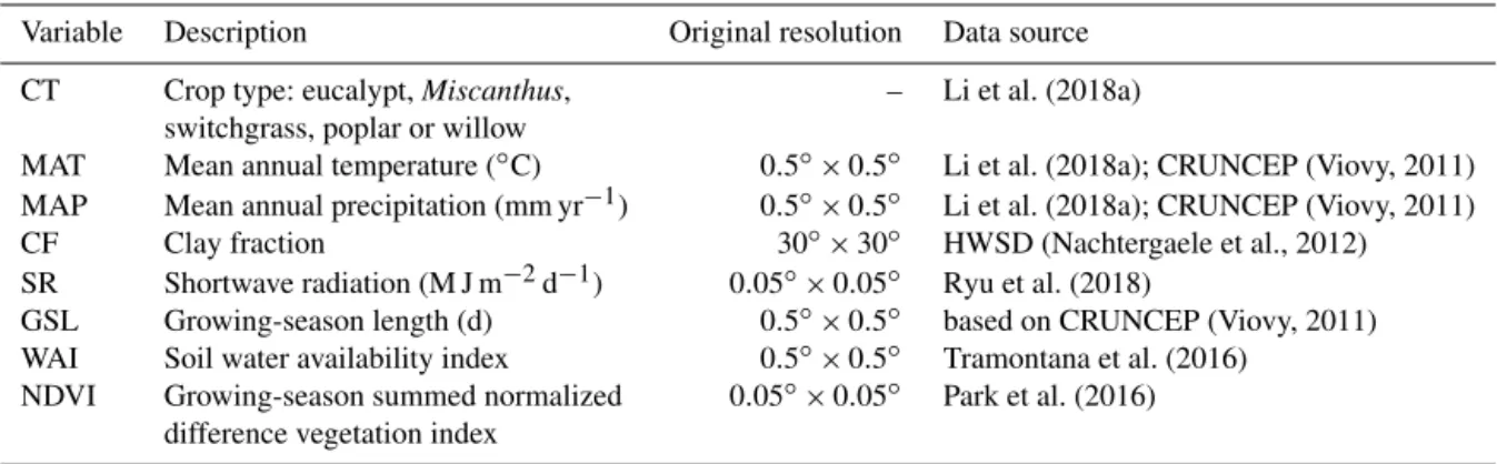
Table 1.Variables used in the upscaling of bioenergy crop yields.
Variable Description Original resolution Data source CT Crop type: eucalypt, Miscanthus, – Li et al. (2018a)
switchgrass, poplar or willow
MAT Mean annual temperature (◦C) 0.5◦×0.5◦ Li et al. (2018a); CRUNCEP (Viovy, 2011) MAP Mean annual precipitation (mm yr−1) 0.5◦×0.5◦ Li et al. (2018a); CRUNCEP (Viovy, 2011) CF Clay fraction 30◦×30◦ HWSD (Nachtergaele et al., 2012) SR Shortwave radiation (M J m−2d−1) 0.05◦×0.05◦ Ryu et al. (2018)
GSL Growing-season length (d) 0.5◦×0.5◦ based on CRUNCEP (Viovy, 2011) WAI Soil water availability index 0.5◦×0.5◦ Tramontana et al. (2016)
NDVI Growing-season summed normalized 0.05◦×0.05◦ Park et al. (2016) difference vegetation index
that include this variable, weighted by the number of sam-ples it splits (Louppe et al., 2013). Although the RF model is robust to correlated explanatory variables, the importance calculation could be biased if there is a strong collinearity between different variables. We thus calculated the correla-tions between all continuous explanatory variables (Table 1) in the training dataset (see Sect. 3.1).
2.2.2 Model training
The workflow of RF training and predicting is shown in Fig. S3. The median yield, MAT, MAP and CF of all site observations for each crop type in each 0.5◦×0.5◦ grid cell from the global yield dataset were calculated to build the training set. That is, for example, several yield observa-tions were reported in the same 0.5◦×0.5◦ grid cell, and the median value of these observations was used for this grid cell. This gives a total of 273 0.5◦×0.5◦ grid cells
with yield observations. The SR, GSL, WAI and NDVI in these grid cells that are not recorded in the yield observa-tion dataset were derived from each corresponding dataset (Table 1) and added in the training set. Crop type (CT; Ta-ble 1) was taken as a categorical variaTa-ble in the RF train-ing and was thus converted to five dummy variables, i.e., CT_eucalypt, CT_Miscanthus, CT_poplar, CT_switchgrass and CT_willow. Taking one yield observation of eucalypt for example, CT_eucalypt was set to 1 and the other four CTs were set to 0. Alternatively, we also tried one RF regression for each individual crop type as a sensitivity test for this cat-egorical variable (see Sect. 4.2).
We first trained the RF model using data from all 273 grid cells. However, the OOB R2 (0.29) is low, indicating the poor performance of the trained model. The low OOB R2 is probably because part of observed yields cannot be ex-plained by the spatially explicit climate and soil conditions used as the explanatory variables in the model training. For example, some strong genotypes may produce high yields under poor climate conditions, while low yields may be ob-served at some sites with poor soil conditions that are not representative of the whole 0.5◦×0.5◦grid cell. In order to
derive the best RF model for prediction, therefore, we further adopted a leave-one-out method (Siewert, 2018; Tramontana et al., 2015). Specifically, RF models were trained each time by excluding one grid cell in the training set. The RF model was then used to predict the yield for this excluded grid cell. The comparison between observations and predictions is shown in Fig. S4. There are 112 grid cells with predicted yields that are biased by more than 1σ of the observed yields (gray dots in Fig. S4a). These strongly biased grid cells were masked and the remaining 161 grid cells retained to train the RF model again to obtain the best RF model. The predicted yields from the best RF model agree well with the observa-tions (Fig. S4b), and R2of the OOB validation is 0.63. Note that the OOB R2 (0.63) serves as an evaluation of the RF model performance rather than the R2 between predictions and observations in the training set (0.95; Fig. S4b). In the RF model training, one can always get a very high R2for the training set by expanding the tree depth, but in that case, the RF model will be overfitted and thus have a poor ability to predict, suggested by a low OOB R2.
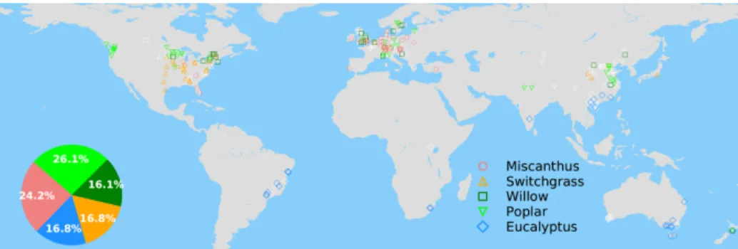
The spatial distribution of the selected grid cells for model training is shown in Fig. 1. There is good observation cover-age in the US, Europe, China, southeastern Brazil and south-ern Australia, but sites are sparse in other regions (Fig. 1). Eucalypt, Miscanthus, switchgrass, poplar and willow take 16.8 %, 24.2 %, 16.8 %, 26.1 and 16.1 % of the total number of selected sites in the training data (Fig. 1).
2.2.3 Model prediction
After training by data from the selected 161 grid cells, the derived RF model was used to predict the global distribu-tion of bioenergy crops yields. Specifically, the gridded val-ues of continuous explanatory variables on each 0.5◦×0.5◦ land grid cell were derived from data sources listed in Ta-ble 1. Five predictions were made, each with one individual prescribed bioenergy crop type (e.g., CT_eucalypt = 1 and the other four CTs are 0 for eucalypt).
Although there are some drought- and/or cold-tolerant Eu-calyptusspecies, most species have a limited cold tolerance
Figure 1.Map of grid cells with yield observations in the global yield dataset. The colored and white markers indicate the selected (blue dots in Fig. S4a) and masked (gray dots in Fig. S4b) grid cells, respectively, based on a bias threshold of 1σ for the RF modeling of these yields. The inset pie plot shows the percentages of each bioenergy crop type in the selected grid cells (colored markers) for model training.
and relative high demands for water and are thus usually cultivated in tropical and warm temperate regions (Jacobs, 1981). Also, because the RF model has a poor ability to ex-trapolate when the values of explanatory variables are out-side the ranges of training data, we only limited each crop prediction to the areas that are adequate for growth. Specifi-cally, the minimum MAT and MAP over all grid cells in the training dataset were derived for each crop. The regions ad-equate for growth of each bioenergy crop were then defined as grid cells with MAT and MAP higher than the minimums in the training data. In another word, if either MAT or MAP in a grid cell is lower than the minimums where a crop type is grown in the training data, this grid cell is excluded for upscaling the yield of this crop. The grid cells with adequate growth conditions for each bioenergy crop type are shown in Fig. S5a–e. We also provided an integrated map (Fig. S5f) where at least one bioenergy crop type can grow to represent the grid cells that can have yield predictions.
Beyond the five predictions made for each bioenergy crop, we derived a prediction of the “best crop” by selecting the bioenergy crop with highest yield in each grid cell to indicate the maximum achievable yields (see Sect. 3.2).
2.3 Bioenergy crop yield maps in IAMs
We compared our derived yield maps from RF with the bioenergy yields from three IAMs: IMAGE (Stehfest et al., 2014), MAgPIE (Popp et al., 2014) and GLOBIOM (Havlík et al., 2011). The yields used in IMAGE and MAgPIE are simulated by a DGVM – LPJmL (Beringer et al., 2011) – and have separate yield data for woody (representing poplar, willow and eucalypt) and herbaceous (representing switch-grass and Miscanthus) bioenergy crops. For comparison, we used the present-day (2010) actual yield maps (derived from RF).
In the IMAGE integrated assessment model framework (Stehfest et al., 2014), the LPJmL model is an integral com-ponent for crop and grass yields, hydrology, dynamic vege-tation, and carbon dynamics (Müller et al., 2016). Bioenergy crop yields for sugarcane, maize, and herbaceous and woody
crops are represented on the grid level in LPJmL and rep-resent potential yields under current technology. In the IM-AGE land model, these potential yields are calibrated on the regional level to currently observed yields based on Gerssen-Gondelach et al. (2015) for the present day. Future projec-tions of bioenergy crop yield depend on scenario-specific as-sumptions of technological progress (Daioglou et al., 2019), but the yield map used in this study is for year 2010 and with-out future yield improvements.
The yield map for year 2010 from MAgPIE used for com-parison in this study includes the yield improvements due to technological development from 1995 to 2010. In the yield maps used as an input to MAgPIE, the potential bioenergy crop yields simulated by LPJmL (Beringer et al., 2011) were reduced using information about observed land-use intensity (Dietrich et al., 2012) and agricultural area (FAO, 2013) be-cause MAgPIE aims to represent actual yields (Bonsch et al., 2016; Humpenöder et al., 2014). It is assumed that LPJmL bioenergy yields represent yields achieved under the highest currently observed land-use intensity, which is observed in Europe. Therefore, LPJmL bioenergy yields for all other re-gions than Europe are reduced proportionally to the land-use intensity in the given region. In addition, yields are calibrated at the regional level to meet the Food and Agriculture Organi-zation of the United Nations (FAO) agricultural area in 1995, resulting in a further reduction of yields in all regions. MAg-PIE bioenergy yields can exceed LPJmL bioenergy yields over time as endogenous investments in R&D (research and development) push the technology frontier.
The bioenergy crop yield map used in GLOBIOM rep-resents the yields from short-rotation tree plantations (i.e., Eucalyptus, Acacia, Gmelina, Betula, Populus, Salix) and thus only woody bioenergy crops. To generate this map, field-measured yields (i.e., as mean annual increments of stem wood) for different short-rotation tree species with proper management practices were first collected from var-ious databases (dated between 1984 and 2006 and sourced from different global regions) and then upscaled to a global yield map based on the spatial patterns of potential net
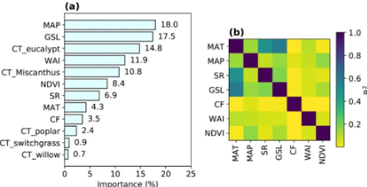
pri-Figure 2.Variable importance in the trained RF model (a) and R2 from the regressions between different explanatory variables (Ta-ble 1) in the training data (b). The importance of one varia(Ta-ble is cal-culated based on the sum of the number of splits across all trees that include this variable, weighted by the number of samples it splits. The relative contributions of each explanatory variable (summed to 100 %) are shown here.
mary productivity (NPP) from Cramer et al. (1999). The es-timation of area potentials for tree plantations in the GLO-BIOM maps followed an approach similar to the one pro-posed by Zomer et al. (2008), including thresholds of tree growth based on aridity, temperature, elevation, population density and existing land cover (Havlík et al., 2011).
3 Results
3.1 Explanatory variables importance
The importance of explanatory variables to the RF model is shown in Fig. 2a, indicating their contributions to the overall tree splits in the forest. We verified that spatial R2 is gen-erally low between any pair of variables (median R2=0.06; interquartile range – IQR = 0.14), with a maximum R2of 0.6 between MAT and GSL (Fig. 2b).
MAP is the most important variable in the RF regres-sion, with a contribution of 18.0 % to the overall tree splits. Another water-related variable, WAI, derived from a simple-bucket model with rainfall and evapotranspiration (ET) datasets, also has a significant contribution (11.9 %), but we note here that ET from observations over natural and cultivated systems may be different from ET in a world with large areas covered by bioenergy crops. The second most im-portant variable is GSL, contributing 17.5 % to the tree splits. However, it should be noted that the correlation between GSL and MAT is relatively high (R2=0.6; Fig. 2b) because GSL was calculated using daily temperature. The contribu-tions of GSL and MAT (4.3 %) may thus be not well sep-arated because of the collinearity, but this did not influence the prediction because RF prediction is not sensitive to the collinearity of explanatory variables. Nevertheless, it implies that temperature-related variables are also very important for predicting the bioenergy crop yields in addition to MAP and WAI. Overall, water-related and temperature-related
vari-ables (MAP, WAI, GSL and MAT) are the most impor-tant variables, together representing an importance level of 51.7 %.
Among bioenergy crop type dummy variables used in the RF model, CT_eucalypt and CT_Miscanthus have marked contributions (14.8 % and 10.8 %), while the contributions from other crop types (CT_poplar, CT_switchgrass and CT_willow) are low (< 3 %; Fig. 2a). This reflects the fact that eucalypt and Miscanthus are generally more productive than others (Li et al., 2018a). The total importance of all bioenergy crop types indices is 29.6 %.
NDVI, as a proxy of maximum plant productivity in each grid cell (Sect. 2.1), and SR contribute 8.4 % and 6.9 % to the trained RF model. CF, as the only soil property used in the regression, has a minor contribution of 3.5 % (Fig. 2a), indicating that soil conditions may have little impact on the bioenergy crop yields. However, this should be interpreted cautiously, considering the mismatch between CF from the HWSD dataset and from the yield observation dataset based on field measurements (Fig. S1c).
3.2 Predicted climate-limited yields
The spatially explicit yield maps of different bioenergy crops were predicted based on the climatic and soil conditions in each grid cell (Fig. 3). MAP is the most important variable in the RF regression (Fig. 2a), and thus the predictions largely depend on the spatial patterns of annual rainfall. This is con-sistent with previous studies in which MAP is the main pre-dictor of NPP across spatial gradients (Knapp et al., 2017). Although the general spatial patterns seem similar, there are still differences caused by other factors than MAP. In gen-eral, eucalypt and Miscanthus have higher yields than the other three bioenergy crops (poplar, willow and switchgrass). The global median yields of eucalypt and Miscanthus in the considered regions are 16.0 (4.1; IQR of grid cells adequate for growth, same below) and 15.3 t DM ha−1yr−1 (2.0 tons of dry matter – DM; Fig. 3a, b). The spatial distributions of predicted yields for poplar, willow and switchgrass show a similar pattern (Fig. 3c–e) because of the low importance of these three crop types in the RF regression (Fig. 2a). Still, the global median yields are slightly different, i.e., 10.1, 10.6 and 10.3 t DM ha−1yr−1 (1.7, 1.7 and 1.6 t DM ha−1yr−1, re-spectively) for poplar, willow and switchgrass, respectively, mainly due to the difference in areas that are adequate for growth (Fig. S5).
The global median yield of the best bioenergy crop is 16.3 t DM ha−1yr−1 (7.0 t DM ha−1yr−1), with the highest yields in the Amazon area and southeastern Asia (Fig. 3f). Consistent with the high yields of Miscanthus and eucalypt, they are the main compositions of the best crop globally, oc-cupying 41.3 % and 35.9 % of the total grid cells that are ad-equate for bioenergy crop growth (Fig. 3g). Eucalypt domi-nates as being the best crop in the wet tropical regions, while Miscanthusdistributes dominantly in the dry tropical regions
Figure 3.Spatial distribution of predicted yields for different bioenergy crops (a–f) and best crop type in each grid cell that is adequate for growth (g). The inset pie plot in (g) shows the fractions of grid cells occupied by each bioenergy crop type. The white areas indicate regions where no prediction was derived due to inadequate conditions defined by minimum temperature and precipitation (see Sect. 2).
and the temperate regions. Willow is the best crop in only 21.2 % of the total grid cells, mainly in the regions with more severe conditions where other crops are excluded for growth based on the MAT and MAP ranges. The fractions of poplar and switchgrass are very low (Fig. 3g), indicating that they are not as competitive as the other crops in term of yields.
Maps of yield differences between eucalypt and Miscant-husand among the other three crops are shown in Fig. S6. There are substantial differences between the yields of euca-lypt and Miscanthus. The higher yields of eucaeuca-lypt than Mis-canthusin South America, the eastern US, central Africa and southeastern Asia and lower yields in other regions (Fig. S6a) can also be reflected by the best crop type in Fig. 3g. Be-cause the contribution of crop types (poplar, switchgrass and willow) is low in the trained random-forest algorithm (CT_poplar, CT_switchgrass and CT_willow in Fig. 2a), the predicted yields in the regions where all three crops can grow are controlled by other mutual variables and thus similar. Therefore, the yield differences among these three crops are mainly caused by the different adequate regions for growth (Fig. S5) defined by the minimum MAT and MAP in the observation dataset. For example, the regions adequate for willow growth include some areas with lower MAP, like the western US, eastern Europe and central Asia (Fig. S5), than for poplar and switchgrass.
3.3 Comparison with maps used in IAMs
The comparison of best bioenergy crop yields in our RF map with the maps used in IMAGE, MAgPIE and GLOBIOM is shown in Fig. 4. The best crop yields refer to the higher yields between woody and herbaceous crops in each grid cell for IMAGE and MAgPIE and the woody crop yields for GLOBIOM, since only short-rotation trees were included in this model. Compared to the RF map, yields are generally lower in the maps used in IAMs (Fig. 4c, e, g), with global median differences of −7.0, −8.1 and −5.2 t DM ha−1yr−1 for IMAGE, MAgPIE and GLOBIOM, respectively. How-ever yields from the IAM maps are higher than the RF map in some regions, e.g., the southeastern US and southeastern Asia for the MAgPIE map (Fig. 4e) and some places in Brazil and northern China for the GLOBIOM map (Fig. 4g). Much lower yields in the IAM maps than the RF map were found in the equatorial winter dry (“Aw” category based on Köppen– Geiger climate classification; Kottek et al., 2006) regions in southeast Brazil, Africa, India and Australia (Fig. 4c, e, g), especially for IMAGE and MAgPIE. In the equatorial full humid (“Af”) and monsoonal (“Am”) regions in South Amer-ica (mainly Amazon region) and AfrAmer-ica (around the Demo-cratic Republic of the Congo), the yield difference is small between the RF and IMAGE and GLOBIOM maps (Fig. 4c, g). In the “Af” and “Am” regions in southeastern Asia,
how-Figure 4.Comparison of bioenergy crop yields between the RF map and maps used in three IAMs (IMAGE, MAgPIE and GLOBIOM). Panels (a, b, d, f) are the best crop yields from each dataset, and the panels (c, e, g) refer to the yield differences between RF and each IAM map (IAM yields minus RF yields where yields are available in both paired maps). The best-crop-yield map from RF (a) is the same as Fig. 3f. The best crop yields in IMAGE and MAgPIE (b, d) are the higher yields between woody and herbaceous bioenergy crops in each grid cell. The best crop yields in GLOBIOM (f) are the yields of woody crops (short-rotation trees), since there is no herbaceous bioenergy crop in GLOBIOM.
ever, yields are lower from GLOBIOM than from RF but similar between IMAGE and RF (Fig. 4c, g). For MAgPIE, yields are systematically lower than those from RF in these tropical regions except southeastern Asia (Fig. 4e). On the other hand, yields from MAgPIE are closest to the RF yields in all the three IAM maps in Europe.
We also showed the best-crop-yield distribution his-tograms from different maps (Fig. 5). Most areas in the RF map have a yield ranging from 15 to 20 t DM ha−1yr−1, and other areas located in another two ranges have yields ranging from 5 to 13 t DM ha−1yr−1and 20 to 24 t DM ha−1yr−1. By contrast, a large fraction of areas from the IAM maps are as-sociated with yields lower than 15 t DM ha−1yr−1 (Fig. 5). This is consistent with the generally higher yields in the RF map than the IAM maps in Fig. 4. In fact, the median mean yield in the regions where yields are available in the four datasets (the overlapped regions between Fig. 4a, b, d, f) from RF is > 50 % higher than the median yields from IAM maps (80 %, 83 % and 59 % for IMAGE, MAgPIE and GLOBIOM, respectively). The shapes of yield distributions among IAMs are also different (Fig. 5). There are more areas with yields below 7 and above 20 t DM ha−1yr−1in the
IM-AGE and MAgPIE maps than the GLOBIOM map. This is also reflected by the higher IQR from IMAGE (IQR = 9.1) and MAgPIE (8.7) than GLOBIOM (5.7 t DM ha−1yr−1). Although both IMAGE and MAgPIE yield maps are based on LPJmL, there are slight differences due to the calibration of the original potential yields of LPJmL to actual yields. Compared to IMAGE, MAgPIE has more areas with yields below 12 DM ha−1yr−1but fewer areas with yields between 17 and 22 DM ha−1yr−1(Fig. 5).
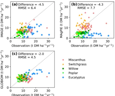
Yields from the IAM maps were also compared directly with yields from field site observations (Fig. 6) that were used to train the RF model (Fig. S4b). Consistent with the global results (Figs. 4, 5), yields from the three IAM maps were lower at most sites (median difference is −4.5, −4.3 and −2.0 DM ha−1yr−1, respectively; Fig. 6a–c). Yields from IMAGE are roughly consistent with the site observa-tions for switchgrass but much lower for Miscanthus and eu-calypt (Fig. 6a). In MAgPIE, herbaceous crops’ (Miscanthus and switchgrass) yields lie around the 1 : 1 line, but woody crops’ (eucalypt, poplar and willow) yields are generally lower than the site observations (Fig. 6b). Because the bioen-ergy crops in the GLOBIOM maps refer to short-rotation
Figure 5.Histograms of best crop yields in our RF yield map and yield maps used in the three IAMs. Only regions where yield values are available in all the four maps are used to generate the histogram.
Figure 6.Comparison of yields from random-forest (RF) and IAM yield maps with site observations used to train the RF model (see the spatial distribution of sites in Fig. 1). Dashed lines indicate the 1 : 1 lines. The median differences and root-mean-square errors (RM-SEs) between site observations and yields from RF and IAMs are also shown.
trees, the yields are similar to the field measurements of wil-low and poplar (also switchgrass) but much wil-lower compared to the observed yields of Miscanthus and eucalypt (Fig. 6c).
In addition to the comparison of the best crop yields, we also showed the yields of woody and herbaceous crops in each dataset, respectively (Fig. S7). Yields of woody bioen-ergy crops in the IAM maps are lower than those in the RF map, especially for IMAGE and MAgPIE. By contrast, the herbaceous crop yields from IMAGE and MAgPIE are close to the RF yields in some regions like the Amazon and south-eastern Asia.
4 Discussion
4.1 Yield comparison with other studies
Our estimated global median yields (Fig. 3) are generally within the ranges summarized by Searle and Malins (2014) from field measurements in the literature for five second-generation bioenergy crops: 0–51, 5–44, 0–35, 0–21 and 1– 35 t DM ha−1yr−1, respectively, for eucalypt, Miscanthus gi-ganteus, poplar, willow and switchgrass. The yields from RF also agree with the yield ranges of several bioenergy crop species (e.g., Miscanthus giganteus, Panicum virgatum, Salix, Populus) based on published yield data (Laurent et al., 2015).
For Miscanthus and switchgrass, there are only small-scale experimental plots in different regions and no large-scale plantation, so no region- or country-large-scale inventory data are available for comparison. Most yield data at farm levels were already included in our observation yield dataset (see “Field_type” and “Field_size” in Table 2 in Li et al., 2018a).
For poplar, willow and eucalypt, we collected some in-ventory data of mean annual increment (MAI) for species of Eucalyptus, Populus and Salix for each country (Table S1, extracted from Table 6a in FAO, 2006). The volume unit of MAI was converted to the mass unit of yield based on the wood density of different tree types (Engineering ToolBox, 2004). The main difficulty is, however, the lack of spatially explicit data about where are plantations located in national-scale inventory data, preventing an accurate comparison with the RF-predicted yields. Still, we derived the yield range in the whole country from the RF-predicted yield maps and compared them with the yield range from the inventory data (FAO, 2006; Fig. S8). Most yield ranges from the inventory data overlapped with the ranges from RF maps (e.g., euca-lypt and willow in Argentina), although the former is gener-ally lower than the latter (Fig. S8). The higher minimum and maximum yields from RF could be caused partly by the ex-clusion of regions with MAP and MAT below the minimums from the observation dataset (to avoid out-of-range predic-tion). Especially in some large countries, the inventory data may have plantations in some harsh climates and soils (e.g., most eucalypt plantations distribute in drier areas in southern Brazil). However, we must note that it is not a fair compar-ison without knowing the exact plantation locations in each country.
4.2 Sensitivity tests and uncertainties in the RF model
We trained RF models using climatic and soil variables and observed yields at a resolution of 0.5◦×0.5◦. However, cli-mate and soil conditions at the observation sites may not match the mean values in the corresponding 0.5◦grid cell. In addition, the number of observation sites in a grid cell may also influence the derived median yields in this grid cell
be-cause of the possible sampling biases (e.g., all observations concentrating in a very small place that is not representative of the whole grid cell). We thus tried to train the model at a resolution of 0.01◦×0.01◦using high-resolution MAP and MAT from WorldClim (Hijmans et al., 2005), but the OOB R2did not improve. We also tried using shortwave incom-ing radiation from CRUNCEP (Viovy, 2011) instead of that from Ryu et al. (2018). SR from CRUNCEP was simply con-verted from the cloudiness provided by CRU based on the calculation of clear-sky incoming solar radiation as a func-tion of date and latitude of each pixel (Viovy, 2011). By con-trast, SR data from BESS were computed based on a series of forcing data from Terra and Aqua MODIS Atmosphere and Land products, including solar zenith angle, dark-target and deep-blue combined aerosol optical depth, cloud opti-cal thickness, cloud top pressure, cloud top temperature, sur-face pressure and sursur-face temperature, total column precip-itable water vapor and total ozone burden, and land surface shortwave albedo (Ryu et al., 2018). The SR data from BESS were also highly consistent with the observational field data (R2=0.95; see Fig. 2 in Ryu et al., 2018). We still tested the RF performance using SR from CRUNCEP, and the OOB R2remained unchanged (0.63), possibly due to the relatively low contribution of SR in the random-forest training (Fig. 2a) and the high spatial correlation between SR from BESS and from CRUNCEP.
We also tried growing-season integrated climate variables instead of annual mean values, but there is no significant im-provement in the model training. Therefore, we focused our analyses on 0.5◦×0.5◦grid cells using mostly mean annual values, since the yield dataset only reported MAP and MAT (no growing-season integrated values) from observations. In addition, the soil properties from HWSD are also highly un-certain (Fig. S1c), and the coarse resolution may not be able to represent the local soil conditions, partly explaining the low importance of CF in the RF model (Fig. 2). More detailed local soil property maps could help to improve the CF impor-tance and thus the corresponding RF model performance.
We replaced the model-derived WAI with satellite-based surface soil moisture (SM) data, including the mean annual soil moisture data from the Soil Moisture and Ocean Salinity (SMOS) satellite during 2010–2018 (Li et al., 2020) and the Soil Moisture Active Passive (SMAP) satellite during 2015– 2018 (O’Neill et al., 2019). The OOB R2 for SMOS and SMAP are 0.60 and 0.59 respectively, compared to the orig-inal value of 0.63. The lower performance may be caused by the fact that satellite-based soil moisture data only accounted for soil water status in the top centimeters, whereas produc-tivity is influenced by root-zone soil moisture. In addition, the importance ranking changed from no. 4 for WAI (Fig. 2a) to no. 8 for SM_SMOS and SM_SMAP (Fig. S9). The rela-tive order of other variables remains unchanged.
Although the total number of 0.5◦×0.5◦grid cells (161) for RF training is relatively small compared to the global to-tal land grid cells (> 60 000), the spatial representativeness of
the sample is more important when being used to upscale the whole population pattern. As shown in Fig. S10, our train-ing sample (gray) covers most ranges of climate and soil variables in the regions that we predicted (pink), implying that our training data are representative of the global ade-quate regions for bioenergy crop growth and thus appropri-ate for upscaling. In addition to the range, the distributions also match well between the training sample and the predic-tion region. Although the distribupredic-tions of shortwave radia-tion are different, the importance of this variable in the RF model is low (Fig. 2a). Furthermore, to avoid possible biases induced by out-of-range prediction, we only limited our pre-dictions in regions with MAT and MAP above the minimums in the training data (Sect. 2.2.3). Thus, this gives us 33 216 grid cells in the prediction regions (instead of > 60 000 glob-ally) and avoids biased predictions in regions that are beyond the capacity of our trained random-forest model. Lastly, we would like to emphasize that the bioenergy crop yield obser-vations were found in published articles or reports in several literature databases and systematically collected (Li et al., 2018a), so it is impossible to include more grid cells (cur-rently 273 0.5◦grid cells – 161 after selecting), as there are no more observations available. Using these data, the OOB R2that serves as an evaluation of the trained random forest is 0.63, implying the trained RF algorithm is acceptable for prediction.
The temporal resolution and coverage of the training dataset are important for training the machine-learning model given the temporal variations in climate conditions. Therefore, we analyzed the sampling time in the training dataset; ∼ 30 % of the yield observations do not have a re-ported sampling year in the original dataset as well as ∼ 30 % in the aggregated 0.5◦×0.5◦ data used for random-forest
training. We thus arbitrarily set 2 years before the publication year as the sampling year for the yield observations with-out reported sampling years (e.g., setting 1997 as the sam-pling year if the reference paper was published in 1999). The frequency of the sampling years in the 0.5◦data used for random-forest training is shown in Fig. S11. The sam-pling years range from 1969 to 2016, with a median year of 1999. We then derived temperature (T ), precipitation (P ) and shortwave radiation (SW; from CRUNCEP because BESS SW starts from 2001) and soil water availability index (WAI) at the sampling year for each grid cell and re-trained the ran-dom forest (RF). However, the OOB R2is 0.54, lower than the original value of 0.63. Possible reasons may include the following: (1) RF training may largely respond to the spatial gradients of climate and soil conditions, and thus the con-tribution of temporal variation may be low, and (2) climate conditions for the sampling year may be a good predictor of yields for annually harvested herbaceous crops, but yields of woody crops like eucalypt, poplar and willow may also be impacted by the previous years in the whole growing cycle. Unfortunately, only about 18 % of the observations have both a reported harvest year and age, impeding the derivation of
the mean climate conditions during the whole growing cy-cle. In addition, using the climate conditions at the sampling years also changed the variable importance (Fig. S12) com-pared to the original one (Fig. 2a). Precipitation is no longer an important contributing variable, while contributions of the other variables are more or less similar to those in the original trained RF.
Management factors like fertilization, irrigation, species and harvest time are important for bioenergy crop growth and impact the yields (Karp and Shield, 2008; Miguez et al., 2008). In the RF model training and prediction, however, we only used spatially explicit climatic conditions, clay frac-tion and crop type as explanatory variables, and other fac-tors (e.g., management drivers) were not included because these explanatory variables are not available on a gridded ba-sis. This may partly be responsible for the moderate OOB R2 (0.63) in the model training. One other reason for the difficulty in taking management into account is the incom-plete information reported for this variable from field mea-surements and thus in the yield observation dataset (Li et al., 2018a). For example, 75 % of the observations did not re-port irrigation information (Li et al., 2018a). Another reason is that different management practices are difficult to harmo-nize. For example, fertilization may be applied annually, only one time at a plantation or irregularly (Li et al., 2018a); there are not enough data samples further classifying crop types (e.g., species or genotypes). Specific to the resolution of our analyses, it is difficult to derive a median or mean manage-ment quantification for a 0.5◦grid cell from all observations inside. In addition, crop age is an important factor in pre-dicting the yields because of the growth cycle of perennial crops like Miscanthus (Lesur et al., 2013). However, the yield data in the observation datasets mainly refer to mean annual biomass yield, which blended the growth cycle, especially for the trees (Li et al., 2018a). In the field measurement stud-ies, biomass yield for trees is often calculated by the total biomass divided by age, although some studies may report the biomass increment at a certain age. Also, because only about one-third of observations have age information and we only aimed to produce a spatially explicit map, age is not used as an explanatory variable in the RF model.
We attempted a RF model training by including an irri-gation flag (yes or no), fertilization flag (yes or no) and/or fertilization frequency (annual or one time). However, these attempts failed to improve the model, and the importance of these factors was very low (< 1 %). The nitrogen application rate reported in the yield observation dataset was also taken as a continuous variable in the exploring RF model training, but it only contributed < 4 % to the total tree splits. Reasons for the low contribution of fertilization (flag, frequency or application rate) may include unknown basic nutrient avail-ability from soils, the possible existence of nitrogen-fixing bacteria, and dry and wet nitrogen depositions. In addition, the yield response of Miscanthus to fertilizer application may not be significant (Cadoux et al., 2012; Heaton et al., 2004).
We took the bioenergy crop type (CT in Table 1) as a cat-egorical variable in our RF model to include yield data from all crops in order to make full use of the climate gradient formation in the upscaling. However, this mixes climate in-formation from one crop with the other crops and may induce some uncertainties. We thus trained one RF model for one in-dividual bioenergy crop, and the OOB R2is 0.42, 0.02, 0.43, 0.19 and 0.42 for eucalypt, Miscanthus, poplar, willow and switchgrass, respectively. The OOB R2for individual crops is lower than the OOB R2 of the original RF model using all crops (OOB R2=0.63, Sect. 2.2.2), especially for Mis-canthus and willow, probably because of the limited num-ber of observations. Still, we mapped the yields for each in-dividual crop with an OOB R2greater than 0.4 (i.e., euca-lypt, poplar and willow) and compared them with our origi-nal estimates (Fig. S13). Although there are some small dif-ferences for poplar and switchgrass, this barely influences our best crop results, since poplar and switchgrass are the highest-yielding crops in only 1.6 % of the cells (Fig. 3g). For eucalypt, our original estimates are higher than the yield predictions from the individual crop (eucalypt) RF model in northwestern Brazil and southeastern Asia but lower in other regions in Brazil and in the temperate regions (Fig. S13). The overall relative differences, however, are small for eu-calypt, with median positive and negative values of 4.0 % (IQR = 11.0) and −7.2 % (5.6 %), respectively.
The prediction of the RF model tends to be not reliable for predictors out of the training data range, and such extrapo-lation should be considered to be inaccurate. We thus com-pared the distributions of variables in the training data and the global data used for prediction and provided the ranges for each bioenergy crop type in the training data (Fig. 10). Because we limited our predictions in the regions that are adequate for bioenergy crop growth using minimum MAT and MAP from observations (Sect. 2.2.3), the distributions of variables used for predictions largely overlapped the distri-butions from the training data (Fig. S10), implying that most of the predictions are reliable without extrapolations out of ranges. Although SR from 20 to 25 MJ m−2d−1is not pre-sented in the training data (Fig. S10), the importance of SR in the RF model is relatively low (Fig. 2a), and thus the in-fluence on our predictions is expected to be small. We should note that only minimum MAT is used to define the adequate regions, but some high-temperature stress (e.g., through heat, vapor pressure deficit or summer drought) could also limit the growth. Although this is not explicitly considered in this study, the area with MAT higher than the maximum MAT in the training data is very small (Fig. S10).
Our predictions are based on the current climate and CO2
level, and thus the future climate changes and CO2
fertil-ization effects are not included. The photosynthetic pathway for C4 plants (such as Miscanthus and switchgrass) is closer to optimal levels of CO2 with present-day atmospheric
lev-els. The CO2 effect could result in large increases in
bioen-ergy crop yield responses to CO2are very sparse, although
this is being addressed in current field studies (e.g., Norby et al., 2016). We adopted a space-for-time approach and an-alyzed the spatial relationship between yields and temper-ature (Fig. S14) to account for the possible yield changes in response to future temperature changes due to adapta-tion. Yields are positively correlated with temperature for all bioenergy crops (Fig. S14; correlations with other explana-tory variables are shown in Figs. S15–20). Miscanthus has the strongest response to temperature, with an increasing rate of 0.41 t DM ha−1yr−1 ◦C−1. Eucalypt and willow have a similar increasing rate (0.27 and 0.26 t DM ha−1yr−1 ◦C−1). The temperature sensitivities of yields are lower for poplar and switchgrass (0.14 and 0.18 t DM ha−1yr−1per◦C). The overall yield response to temperature for the best crop is 0.42 t DM ha−1yr−1 ◦C−1(Fig. S14). It is higher than each individual crop because it combined the yield gradient from multiple crops, so the yield sensitivities to temperature for the best crop also comprise possible transitions of the low-yield crop type to the high-low-yield type. Based on an increase of 0.9◦C from the preindustrial period until now (Millar et al., 2017), the temperature sensitivity of the best crop implies a mean increase of 0.46 t DM ha−1yr−1in yields from present day to 2100 in the 2◦C temperature increase scenario. How-ever, this is just a simple extrapolation based on spatial gra-dients and should be interpreted cautiously. For example, a future increase in soil aridity could cause soil degradations and counteract the yield increases due to CO2 fertilization
and temperature increase (Balkoviˇc et al., 2018).
4.3 Comparison with other yield maps
One potential application of our RF yield maps is to be used as an input to IAMs, so we made detailed comparisons with the currently used yields maps in three IAMs in terms of spatial patterns (Fig. 4), yield distributions (Fig. 5) and site-level yields (Fig. 6). Yields from the IAM maps are gener-ally lower than those from our derived RF maps (Figs. 4, 5) and the site-level field observations (Fig. 6). One possible reason is that the IMAGE and MAgPIE models calibrated the simulated potential yields of LPJmL (highest yield that can be achieved by the best management practices currently available) to the actual yields (see Sect. 2.3). The field obser-vations are usually under some degree of management like irrigation or fertilization, and are thus close to the poten-tial yields, so IAMs reduced the yields using a calibration factor to represent the gap between the potential and actual yields, as the potential yields may not be reached in reality, especially in some low-income countries. As another con-sequence of using data from well-managed field trials, the predicted yields from the RF model could be higher than the practical yields in large-scale plantations. Most of the obser-vations in the training data are from small-scale experimen-tal trials with management practices rather than real farmers’ fields (Li et al., 2018a). In addition, some yield observations
are based on harvests at the peak yield time in summer or autumn rather than in winter or early spring after leaf fall and drying in practice. In fact, Searle and Malins (2014) re-viewed bioenergy crop yields in the literature and concluded that there are significantly lower yields in semi-commercial-scale trails than small plots because of the biomass drying loss and inefficient mechanical harvest. Crops in small plots may also benefit from the edge effect by receiving more light (Searle and Malins, 2014). However we should note that the median yield in each grid cell with multiple observations is used to the train the RF model, and thus some extremely high yield observations due to intensive management prac-tices may not contribute strongly to the trained RF model.
In addition, inclusion of or more dependence on the high-yield bioenergy crop types (i.e., Miscanthus and eucalypt) in the RF model would also lead to higher yield predictions. For example, in LPJmL, where the IMAGE and MAgPIE yield maps come from, switchgrass and Miscanthus were treated as one single PFT (Beringer et al., 2011; Heck et al., 2016), although these two crop types have very different physio-logical parameters and thus significant difference in yields (Dohleman et al., 2009; Heaton et al., 2008; Li et al., 2018b). The calibration of this one single PFT using both yields’ data from switchgrass and Miscanthus would overestimate yields of the former and underestimate the latter. For euca-lypts, LPJmL seemed to underestimate the yields in the first place (see the comparison with field measurements in Fig. 1b in Heck et al., 2016). The RF model trained in this study, on the other hand, relies more on the crop types of Miscanthus and eucalypt (see their importance in Fig. 2a). Although yield maps from IMAGE and MAgPIE were both based on the LPJmL simulations, they showed some differences in spatial patterns, yield distributions and site-level yield comparison due to different calibration processes for the yield data simu-lated by LPJmL (see Sect. 2.3).
Yields from the GLOBIOM map are close to the site-level observations of willow, poplar and switchgrass (Fig. 6c). Therefore, the lower yields from GLOBIOM than the best crop yields from RF are mainly caused by the inclusion of Miscanthusand more eucalypt observation data in the RF model. More contributions from these high-yield crops drive the yields higher in the RF predictions.
Accurate input data of bioenergy crop yields are crucial for IAMs to simulate the future land-use change through the trade-off between BECCS and other climate mitigation op-tions. The global median yields from our RF map are > 50 % higher than those used in IAMs in the overlapped regions (Fig. 5). Therefore, if our RF yield data are used in IAMs and all the other conditions being equal, it will make the BECCS option more competitive and require less land for bioenergy crop plantation to achieve the same mitigation tar-get, although gaps between predicted yields from RF and ac-tual yields particularly in low-income countries need to be further taken into account. Also, it may need more water and nutrients in order to sustain the high yields. Although
the yield response to fertilizers may be not obvious (Cadoux et al., 2012; Miguez et al., 2008), the net nutrient loss from biomass harvest must be replenished to maintain the nutrient balance in the soil and support further growth.
In addition, we compared the yield map derived from ran-dom forest with the yields simulated by the land surface model – ORCHIDEE (Fig. S21). Because poplar and wil-low were taken as one PFT in ORCHIDEE (Li et al., 2018b), the average yields of poplar and willow from random for-est were used for comparison (Fig. S21b). The yields sim-ulated by ORCHIDEE are generally higher than those from random forest, especially for Miscanthus and poplar and wil-low. This could be largely expected because in this version of ORCHIDEE, there are no nutrient limitations on plant growth, no effect of pests and disease on crops, and the man-agement practices were implicitly included when adjusting the productivity parameters in the model to match the site ob-servations with management like irrigation, fertilization or a specific highly productive genotype. There could be a similar case in LPJmL (Heck et al., 2016), and this could also be why the IAMs calibrated the LPJmL yields based on currently ob-served yields to get the potential yield maps (Sect. 2.3). On the other hand, the predictions from random forest are largely constrained by the yield range of observations, representing the yields that can be achieved (or were achieved during the period when yield data were reported) under current (opti-mal) technology. This is exactly the purpose of producing this data product in our study, which is observation-based and can be used to benchmark the yields simulated by land surface models or IAMs.
5 Data availability
The field observed site-level yield data for major lig-nocellulosic bioenergy crops can be downloaded from https://doi.org/10.6084/m9.figshare.c.3951967 (Li et al., 2018a). The 0.5◦×0.5◦ gridded global maps for yields of different bioenergy crops and the best crop and for the best crop composition generated from the random-forest model in this study can be download from https://doi.org/10.5281/zenodo.3274254 (Li, 2019).
6 Conclusion
We mapped bioenergy crop yields at the global scale using a machine-learning method trained on field yield data and based on several climatic and soil conditions. In addition to evaluating the performances of IAMs and DGVMs, our spa-tially explicit bioenergy crop yields can also be used to de-termine the suitable lands with proper bioenergy crop yields, conduct life cycle assessment and estimate the nutrient re-moval from biomass harvest. Although there are a large num-ber of field measurements in the yield observation dataset used to build the RF model, the geographic coverage is poor
in some regions. Therefore, more field measurements in re-gions with limited observations (e.g., Africa) and a proper quantification and synthesis of management factors will be useful to improve the predictions of global yields in future.
Supplement. The supplement related to this article is available online at: https://doi.org/10.5194/essd-12-789-2020-supplement.
Author contributions. PC and WL conceived the study. WL an-alyzed the data and drafted the paper. ES, AP, FDF, JD, FH, PH and MO provided the yield maps from IAMs. TP provided the NDVI data. All authors contributed to the interpretation of the results and to the paper.
Competing interests. The authors declare that they have no con-flict of interest.
Acknowledgements. Wei Li acknowledges the European Commission-funded project LUC4C (grant no. 603542). Philippe Ciais acknowledges support by the CLAND Convergence In-stitute of the French Agence Nationale de la Recherche under the “Investissements d’avenir” programme with the reference ANR-16-CONV-0003. Anna B. Harper acknowledges funding from the Engineering and Physical Sciences Research Foundation (EPSRC) Fellowship EP/N030141/1 and Natural Environment Research Council (NERC) grant NE/P019951/1. Taejin Park acknowledges support from NASA’s Carbon Monitoring System program (80NSSC18K0173-CMS). Wei Li and Philippe Ciais are supported by the European Research Council through Synergy Grant ERC-2013-SyG-610028 “IMBALANCE-P”.
Financial support. This study is supported by the National Key Research and Development Program of China (grant no. 2019YFA0606604) and European Research Council Synergy Grant (“IMBALANCE-P” (grant no. ERC-2013-SyG-610028)).
Review statement. This paper was edited by Scott Stevens and reviewed by two anonymous referees.
References
Balkoviˇc, J., Skalský, R., Folberth, C., Khabarov, N., Schmid, E., Madaras, M., Obersteiner, M., and van der Velde, M.: Impacts and Uncertainties of +2◦C of Climate Change and Soil Degra-dation on European Crop Calorie Supply, Earth’s Future, 6, 373– 395, https://doi.org/10.1002/2017EF000629, 2018.
Beringer, T., Lucht, W., and Schaphoff, S.: Bioenergy produc-tion potential of global biomass plantaproduc-tions under environmen-tal and agricultural constraints, GCB Bioenergy, 3, 299–312, https://doi.org/10.1111/j.1757-1707.2010.01088.x, 2011.
Berndes, G., Hoogwijk, M., and Van Den Broek, R.: The contribution of biomass in the future global energy sup-ply: A review of 17 studies, Biomass Bioenerg., 25, 1–28, https://doi.org/10.1016/S0961-9534(02)00185-X, 2003. Bonsch, M., Humpenöder, F., Popp, A., Bodirsky, B., Dietrich, J. P.,
Rolinski, S., Biewald, A., Lotze-Campen, H., Weindl, I., Gerten, D., and Stevanovic, M.: Trade-offs between land and water re-quirements for large-scale bioenergy production, GCB Bioen-ergy, 8, 11–24, https://doi.org/10.1111/gcbb.12226, 2016. Breiman, L.: Random forests, Mach. Learn., 45, 5–32,
https://doi.org/10.1023/A:1010933404324, 2001.
Cadoux, S., Riche, A. B., Yates, N. E., and Machet, J.-M.: Nutrient requirements of Miscanthus x giganteus: conclusions from a re-view of published studies, Biomass Bioenerg., 38, 14–22, 2012. Cai, X., Zhang, X., and Wang, D.: Land availability for
biofuel production, Environ. Sci. Technol., 45, 334–339, https://doi.org/10.1021/es103338e, 2011.
Cramer, W., Kicklighter, D. W., Bondeau, A., Iii, B. M., Churk-ina, G., Nemry, B., Ruimy, A., Schloss, A. L., and The Par-ticipants of the potsdam NPP model intercomparison: Com-paring global models of terrestrial net primary productivity (NPP): overview and key results, Glob. Chang. Biol., 5, 1–15, https://doi.org/10.1046/j.1365-2486.1999.00009.x, 1999. Daioglou, V., Doelman, J. C., Wicke, B., Faaij, A., and van Vuuren,
D. P.: Integrated assessment of biomass supply and demand in climate change mitigation scenarios, Glob. Environ. Chang., 54, 88–101, https://doi.org/10.1016/J.GLOENVCHA.2018.11.012, 2019.
Dietrich, J. P., Schmitz, C., Müller, C., Fader, M., Lotze-Campen, H., and Popp, A.: Measuring agricultural land-use intensity - A global analysis using a model-assisted approach, Ecol. Modell., 232, 109–118, https://doi.org/10.1016/j.ecolmodel.2012.03.002, 2012.
Dohleman, F. G., Heaton, E. A., Leakey, A. D. B., and Long, S. P.: Does greater leaf-level photosynthesis explain the larger solar energy conversion efficiency of Miscanthus relative to switch-grass?, Plant. Cell Environ., 32, 1525–1537, 2009.
El Akkari, M., Réchauchère, O., Bispo, A., Gabrielle, B., and Makowski, D.: A meta-analysis of the greenhouse gas abatement of bioenergy factoring in land use changes, Sci. Rep., 8, 8563, https://doi.org/10.1038/s41598-018-26712-x, 2018.
Engineering ToolBox: Density of Various Wood Species, avail-able at: https://www.engineeringtoolbox.com/wood-density-d_ 40.html (last access: 15 November 2019), 2004.
FAO: Global planted forests thematic study: results and analysis, by: Del Lungo, A., Ball, J., and Carle, J., Planted Forests and Trees Working Paper 38, 2006.
FAO: Statistical database, Rome, Italy, available at: http://www.fao. org/faostat/en/#data (last access: 30 March 2020), 2013. Frich, P., Alexander, L. V., Della-Marta, P., Gleason, B.,
Hay-lock, M., Tank Klein, A. M. G., and Peterson, T.: Ob-served coherent changes in climatic extremes during the sec-ond half of the twentieth century, Clim. Res., 19, 193–212, https://doi.org/10.3354/cr019193, 2002.
Fuss, S., Lamb, W. F., Callaghan, M. W., Hilaire, J., Creutzig, F., Amann, T., Beringer, T., De Oliveira Garcia, W., Hartmann, J., Khanna, T., Luderer, G., Nemet, G. F., Rogelj, J., Smith, P., Vi-cente, J. V., Wilcox, J., Del Mar Zamora Dominguez, M., and Minx, J. C.: Negative emissions – Part 2: Costs, potentials and
side effects, Environ. Res. Lett., https://doi.org/10.1088/1748-9326/aabf9f, 2018.
Gerssen-Gondelach, S., Wicke, B., and Faaij, A.: Assessment of driving factors for yield and productivity developments in crop and cattle production as key to increasing sus-tainable biomass potentials, Food Energy Secur., 4, 36–75, https://doi.org/10.1002/FES3.53, 2015.
Guimberteau, M., Zhu, D., Maignan, F., Huang, Y., Yue, C., Dantec-Nédélec, S., Ottlé, C., Jornet-Puig, A., Bastos, A., Laurent, P., Goll, D., Bowring, S., Chang, J., Guenet, B., Tifafi, M., Peng, S., Krinner, G., Ducharne, A., Wang, F., Wang, T., Wang, X., Wang, Y., Yin, Z., Lauerwald, R., Joetzjer, E., Qiu, C., Kim, H., and Ciais, P.: ORCHIDEE-MICT (v8.4.1), a land surface model for the high latitudes: model description and validation, Geosci. Model Dev., 11, 121–163, https://doi.org/10.5194/gmd-11-121-2018, 2018.
Hastings, A., Clifton-Brown, J., Wattenbach, M., Mitchell, C. P., and Smith, P.: The development of MISCANFOR, a new Miscanthus crop growth model: towards more robust yield predictions under different climatic and soil conditions, GCB Bioenergy, 1, 154–170, https://doi.org/10.1111/j.1757-1707.2009.01007.x, 2009.
Havlík, P., Schneider, U. A., Schmid, E., Böttcher, H., Fritz, S., Skalský, R., Aoki, K., Cara, S. De, Kindermann, G., Kraxner, F., Leduc, S., McCallum, I., Mosnier, A., Sauer, T., and Ober-steiner, M.: Global land-use implications of first and sec-ond generation biofuel targets, Energ. Policy, 39, 5690–5702, https://doi.org/10.1016/j.enpol.2010.03.030, 2011.
Heaton, E., Voigt, T., and Long, S. P.: A quantitative review com-paring the yields of two candidate C4perennial biomass crops in relation to nitrogen, temperature and water, Biomass Bioen-erg., 27, 21–30, https://doi.org/10.1016/j.biombioe.2003.10.005, 2004.
Heaton, E. A., Dohleman, F. G., and Long, S. P.: Meeting US biofuel goals with less land: the potential of Miscanthus, Glob. Chang. Biol., 14, 2000–2014, 2008.
Heck, V., Gerten, D., Lucht, W., and Boysen, L. R.: Is extensive terrestrial carbon dioxide removal a “green” form of geoengi-neering? A global modelling study, Glob. Planet. Change, 137, 123–130, https://doi.org/10.1016/j.gloplacha.2015.12.008, 2016. Hijmans, R. J., Cameron, S. E., Parra, J. L., Jones, P. G., and Jarvis, A.: Very high resolution interpolated climate sur-faces for global land areas, Int. J. Climatol., 25, 1965–1978, https://doi.org/10.1002/joc.1276, 2005.
Hoffman, A. L., Kemanian, A. R., and Forest, C. E.: Analysis of cli-mate signals in the crop yield record of sub-Saharan Africa, Glob. Chang. Biol., 24, 143–157, https://doi.org/10.1111/gcb.13901, 2018.
Humpenöder, F., Popp, A., Dietrich, J. P., Klein, D., Lotze-Campen, H., Bonsch, M., Bodirsky, B. L., Weindl, I., Stevanovic, M., and Müller, C.: Investigating afforestation and bioenergy CCS as cli-mate change mitigation strategies, Environ. Res. Lett., 9, 064029, https://doi.org/10.1088/1748-9326/9/6/064029, 2014.
Jacobs, M. R.: Eucalypts for planting, Food and Agriculture Orga-nization of the United Nations, Rome, 1981.
Kang, S., Post, W. M., Nichols, J. A., Wang, D., West, T. O., Bandaru, V., and Izaurralde, R. C.: Marginal Lands: Con-cept, Assessment and Management, J. Agric. Sci., 5, 129–139, https://doi.org/10.5539/jas.v5n5p129, 2013.