A cloud filtering method for microwave upper tropospheric humidity measurements

(1)

HAL Id: hal-00302829

https://hal.archives-ouvertes.fr/hal-00302829

Submitted on 30 May 2007

HAL is a multi-disciplinary open access

archive for the deposit and dissemination of sci-entific research documents, whether they are pub-lished or not. The documents may come from teaching and research institutions in France or abroad, or from public or private research centers.

L’archive ouverte pluridisciplinaire HAL, est destinée au dépôt et à la diffusion de documents scientifiques de niveau recherche, publiés ou non, émanant des établissements d’enseignement et de recherche français ou étrangers, des laboratoires publics ou privés.

A cloud filtering method for microwave upper

tropospheric humidity measurements

S. A. Buehler, M. Kuvatov, T. R. Sreerekha, V. O. John, B. Rydberg, P.

Eriksson, J. Notholt

To cite this version:

S. A. Buehler, M. Kuvatov, T. R. Sreerekha, V. O. John, B. Rydberg, et al.. A cloud filtering method for microwave upper tropospheric humidity measurements. Atmospheric Chemistry and Physics Dis-cussions, European Geosciences Union, 2007, 7 (3), pp.7509-7534. �hal-00302829�

(2)

ACPD

7, 7509–7534, 2007

Cloud filtering for UTH S. A. Buehler et al. Title Page Abstract Introduction Conclusions References Tables Figures ◭ ◮ ◭ ◮ Back Close

Full Screen / Esc

Printer-friendly Version Interactive Discussion

EGU

Atmos. Chem. Phys. Discuss., 7, 7509–7534, 2007 www.atmos-chem-phys-discuss.net/7/7509/2007/ © Author(s) 2007. This work is licensed

under a Creative Commons License.

Atmospheric Chemistry and Physics Discussions

A cloud filtering method for microwave

upper tropospheric humidity

measurements

S. A. Buehler1, M. Kuvatov2, T. R. Sreerekha3, V. O. John4, B. Rydberg5, P. Eriksson5, and J. Notholt2

1

Lulea Technical University, Dept. of Space Science, Kiruna, Sweden 2

IUP, University of Bremen, Bremen, Germany 3

Satellite Applications, Met Office, Exeter, UK 4

RSMAS, University of Miami, USA 5

Dept. of Radio and Space Science, Chalmers University of Technology, Gothenburg, Sweden Received: 14 March 2007 – Accepted: 14 May 2007 – Published: 30 May 2007

(3)

ACPD

7, 7509–7534, 2007

Full Screen / Esc

EGU Abstract

The paper presents a cloud filtering method for upper tropospheric humidity (UTH) measurements at 183.31±1.00 GHz. The method uses two criteria: The difference between the brightness temperatures at 183.31±7.00 and 183.31±1.00 GHz, and a threshold for the brightness temperature at 183.31±1.00 GHz. The robustness of this

5

cloud filter is demonstrated by a mid-latitudes winter case-study.

The paper then studies different biases on UTH climatologies. Clouds are associated with high humidity, therefore the dry bias introduced by cloud filtering is discussed and compared to the wet biases introduced by the clouds radiative effect if no filtering is done. This is done by means of a case study, and by means of a stochastic cloud

10

database with representative statistics for midlatitude conditions.

The consistent result is that both cloud wet bias (0.8% RH) and cloud filtering dry bias (–2.4%RH) are modest for microwave data, where the numbers given are for the stochastic cloud dataset. This indicates that for microwave data cloud-filtered UTH and unfiltered UTH can be taken as error bounds for errors due to clouds. This is not

15

possible for the more traditional infrared data, since the radiative effect of clouds is much stronger there.

The focus of the paper is on midlatitude data, since atmospheric data to test the filter for that case were readily available. The filter is expected to be applicable also to subtropical and tropical data, but should be further validated with case studies similar

20

to the one presented here for those cases.

1 Introduction

Humidity in the atmosphere, and particularly in the upper troposphere, is one of the major factors in our climate system. Changes in its distribution affect the atmospheric energy balance. It is therefore essential to monitor and study upper tropospheric

hu-25

(4)

ACPD

7, 7509–7534, 2007

Full Screen / Esc

EGU

to traditional direct measurements of atmospheric humidity by radiosondes, satellites provide humidity measurements with global coverage. Satellite measurements of UTH are typically made in two specific frequency regions: in the infrared at 6.3 µm and in the microwave at 183.31 GHz. The infrared instruments are the more established ones, whereas the microwave instruments became available only rather recently.

5

UTH can be retrieved from satellite radiances using an algorithm developed by

So-den and Bretherton (1996). They used a linear relation between the natural logarithm of UTH and brightness temperature (ln(UTH)=a+b∗TB), and derived the fit parameters a and b using linear regression. In this algorithm, UTH is defined as the Jacobian weighted mean of relative humidity in the upper troposphere which is roughly between

10

500 and 200 hPa. Soden and Bretherton(1996) applied the algorithm to infrared data from the HIRS instrument.

One of the available microwave instruments for measuring UTH is the Ad-vanced Microwave Sounding Unit B (AMSU-B) (Saunders et al., 1995). It has three humidity sounding channels centered around a water vapor absorption line at

15

183.31 GHz. These channels have center frequencies of 183.31±1.00, 183.31±3.00, and 183.31±7.00 GHz and are called Channel 18, 19, and 20, respectively. Recently,

Buehler and John(2005) demonstrated that UTH can be derived from AMSU-B Chan-nel 18 brightness temperatures with a precision of 2%RH at low UTH values and 7%RH at high UTH values. The same retrieval algorithm was used for the work described

20

here. We will henceforth refer to the above paper as BJ.

In general, clouds are more transparent in the microwave than in the infrared. There-fore, data from microwave sensors are less contaminated by clouds than data from IR sensors. This is particularly true for Channel 18 of AMSU-B. The signal it receives originates mostly from the upper part of the troposphere. Thus, it is not sensitive to

25

low clouds. However, clouds can affect the measurement if there is a high cloud with a high ice content in the line of sight (LOS) of the instrument. In such a case the radia-tion is scattered away from the LOS by ice particles in the cloud so that the brightness temperature measured by the instrument is colder than it would be without the cloud.

(5)

ACPD

7, 7509–7534, 2007

Full Screen / Esc

EGU

In clear-sky conditions brightness temperatures from Channel 18 (T_B18) are colder than brightness temperatures from Channel 20 (T_B20). This is due to the atmospheric temperature lapse rate, and the fact that Channel 18 is sensitive to a higher region of the troposphere than Channel 20. However, in the presence of ice clouds T_B18 can be warmer than T_B20. Thus, the brightness temperature difference, defined as

5

∆TB=T 20 B −T

18

B can be used to detect the presence of clouds. For example, Adler et al. (1990) showed, using aircraft microwave observations, that ∆TB can reach up to −100 K in a strong convective system andBurns et al.(1997) suggested to use ∆TB<0 as a criterion to filter out convective cloud cases before retrieving water vapor from these measurements.

10

Greenwald and Christopher(2002) investigated the effect of cold clouds (defined as 11 µm brightness temperatures less than 240 K) on T_B18. They concluded that non-precipitating clouds produce on average 5%RH error in UTH retrieval, whereas precip-itating clouds produce 18%RH error. They used infrared data to estimate the clear-sky background T_B18 (which was found to be 242±2 K) in order to estimate this error.

Un-15

fortunately, it is not possible to use the above numbers directly to assess the impact of clouds on a UTH climatology, because the averages refer not to the total number of measurements, but only to all clouds in the given class, where the class definitions are somewhat arbitrary. For example if the non-precipitating cloud class is extended towards thinner clouds, then the average impact of clouds of this class on UTH will

20

appear to be smaller.

Another application of AMSU-B data cloud filtering is given by Hong et al. (2005). The authors used the three AMSU-B sounding channels centered around 183.3 GHz to detect tropical deep convective clouds. They conclude that the deep convective cloud fraction in the tropics is around 0.3%, and that the contribution of overshooting

25

convection to this is around 26%.

In this article we develop a cloud filter that uses only the microwave data, no addi-tional infrared data (Sect.2). This is achieved by combining the approaches from earlier

(6)

ACPD

7, 7509–7534, 2007

Full Screen / Esc

EGU

studies. We use a case study to demonstrate the robustness of the filter (Sect. 3.1). Next, we use the same case study to estimate the bias in the retrieved UTH that is introduced by the cloud filtering, and compare that to the bias introduced by the ra-diative effect of the clouds themselves, if they are not filtered out (Sect. 3.2). In this context, the impact of surface emissions on retrieved UTH and on the cloud filtering

5

procedure must also be discussed (Sect.3.3). Finally, we put the results from the case study on a firmer statistical basis by analyzing the cloud bias and cloud filtering bias for a stochastic dataset of midlatitude cloud cases with realistic statistics (Sect. 3.4). Section4contains a summary and the conclusions of this work.

2 Cloud filter methodology

10

The cloud filter we propose combines a threshold value for T_B18 (240 K for nadir data) and the ∆TB (0 K). To demonstrate this, we use two-dimensional histograms of ∆TB versus T_B18, such as the ones shown in Fig. 1. In the left plot, one month of AMSU-B measurements were used to plot the histogram. The color coded contour levels show the frequency of measurements, normalized relative to the maximum. In other words,

15

the figure shows the combined probability density function (PDF) for T_B18 and ∆TB. The maximum of the PDF is near T_B18=245 K and ∆TB=20 K. Most cases are indeed above T_B18_{=240 K and ∆T}_B_{=0 K. There is a tail of cases with negative ∆T}_B _{as low as −60 K.} We identify these cases mostly with clouds.

In principle, negative ∆TB values can also be an indicator of surface influence on

20

T_B18. Under very dry atmospheric conditions, both channels measure radiation emitted from the Earth’s surface and the atmosphere. If we assume the surface emissivity to be the same for both channels, T_B18 will be warmer than T_B20 because the contribution of atmospheric emission will be more for Channel 18 as the frequencies are closer to the line center.

25

(7)

ACPD

7, 7509–7534, 2007

Full Screen / Esc

EGU

surface effects, a two-dimensional histogram was plotted with brightness temperatures simulated for a clear-sky scenario (not considering clouds in the RT model). The re-sult of this exercise is demonstrated in the middle plot of Fig.1. The brightness tem-peratures used in this figure are calculated with the radiative transfer model RTTOV (Saunders et al.,1999) using ECMWF ERA-40 reanalysis data. The surface emissivity

5

model was FASTEM (English and Hewison,1998) over the ocean, and one of five dif-ferent fixed surface emissivity values, depending on terrain type, over land. Confirming our expectations this figure shows that for clear-sky conditions there are very little data where ∆TB is below 0 K. The simulated clear-sky data in the middle plot also confirms the criterion ofGreenwald and Christopher(2002) that T_B18 should be above 240 K for

10

clear-sky cases, which was not evident from the measured AMSU-B data in the left plot. We conclude that it is valid to use the two criteria in combination as a cloud filter.

While the threshold of 240 K for T_B18 is valid for nadir looking measurements, due to limb darkening this threshold shifts to colder brightness temperatures for off-nadir looking measurements. As shown in the right plot of Fig.1, the depression from nadir

15

to off-nadir is approximately 7 K.

To derive viewing angle dependent values for the T_B18 threshold, we simulated clear-sky AMSU-B measurements for each instrument angle. This simulation was done with a sampled ECMWF data set (Chevallier,2001) using the Atmospheric Radiative Trans-fer Simulator (ARTS) (Buehler et al.,2005). For each viewing angle, minima of T_B18 for

20

a number of ∆TB intervals around the ∆TB threshold were determined. The mean of these minima was taken as T_B18 threshold for that viewing angle. A summary of the threshold values is given in Table1.

Figures similar to Fig.1 were also generated for other latitude ranges (not shown). Overall, they look rather similar. In particular, the assumed threshold values appear to

25

be applicable also for tropical and sub-tropical data. We make no attempt here to fine-tune the filter for these other latitudes, since the focus of the paper is on mid-latitudes.

(8)

ACPD

7, 7509–7534, 2007

Full Screen / Esc

EGU

3 Results and discussion

In this section we demonstrate the cloud filter using a strong ice cloud event over northern midlatitudes. We also estimate the clear-sky bias in the retrieved UTH fields due to cloud screening, and discuss the impact of surface emissions.

3.1 Case study

5

For the case study we used model fields and microwave measurements from a strong ice cloud event that occurred over the UK on 25 January 2002. The model fields are from the Met Office (UK) mesoscale model UKMES (Cullen, 1993). Profiles of pressure, temperature, relative humidity, cloud ice water content and cloud liquid water content were used to simulate AMSU-B radiances.

10

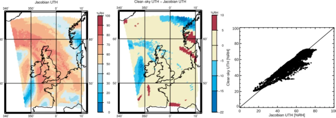
To put the results on the cloud impact in the right perspective, one should keep in mind the properties of the applied UTH retrieval method and its limitations. For this purpose we applied it first to simulated clear-sky brightness temperatures. The results are displayed in Fig.2, which shows the quantities UTH_Jacand UTH_Tbin different ways. The quantity UTHJac is the Jacobian weighted upper tropospheric humidity, calculated

15

from the relative humidity profiles and the AMSU-B Jacobian (for details, see BJ). The quantity UTH_Tb is UTH calculated from the simulated brightness temperatures by ap-plying the coefficients derived by BJ. The humidity unit used here and everywhere in this article is the relative humidity over liquid water (%RH).

The leftmost plot of the figure shows a map of the UTH_Jac field. The middle plot

20

shows a map of UTHTb-UTHJac. The rightmost plot is a scatter-plot of UTHTb versus UTHJac. The figure shows that the retrieval method works well, as most of the differ-ences are within ±5%RH. It is interesting to note where the discrepancies between UTHJac and retrieved UTH, which are referred to as regression noise in BJ, happen. Strong differences of up to 22%RH occur in areas with unusual atmospheric states, for

25

example behind the cold front. In this area, where warm air is over-laying cold air, the temperature and humidity lapse rates are less steep than in the average state, resulting

(9)

ACPD

7, 7509–7534, 2007

Full Screen / Esc

EGU

in a different relation between ln(UTH) and brightness temperature.

Comparing the scatter plot of UTH_Tbversus UTH_Jac with the similar scatter plot pre-sented in BJ, reveals that the differences are in the same order. The map plot reveals that what appears as noise for a set of random atmospheric states, appears as area biases for a real atmospheric scenario, because neighboring atmospheric states are

5

similar. This is the expected behavior of a regression retrieval method.

In addition to these errors from the regression method, a retrieval from real AMSU-B data will contain errors due to a possible contribution by the surface, and due to clouds. The surface effects for this scenario were assessed by repeating the simulations with different surface emissivities of 0.6 and 0.99 for over-land data. UTHTbbetween the two

10

different cases differs by less than 0.4%RH for the investigated scenario which means that surface effects are negligible in this case.

Let us now come to the cloud impact. Figure3 is used to discuss this. The figure is organized in three columns, the leftmost column shows model quantities, the middle column radiances, and the rightmost column cloud induced UTH errors.

15

The top plot in the left column of Fig. 3 shows the ice water path (IWP) field. The bottom plot in the left column shows the cloud top altitude. The model does not provide information on the size distribution of the cloud particles and their shape and orienta-tion. Therefore, it was assumed that all particles have a spherical shape following a size distribution according toMcFarquhar and Heymsfield (1997). This

parametriza-20

tion was chosen out of convenience, and because it is the parametrization used for operational EOS-MLS retrievals (Wu et al.,2006).

The top plot in the middle column of Fig.3shows the measured AMSU-B Channel 18 radiances for this scene. The bottom plot in the middle column shows a simulation of the same scene, based on the model fields. The radiances were simulated with

25

the Atmospheric Radiative Transfer Simulator (ARTS) (Buehler et al.,2005) using the version that can simulate scattering (Emde et al., 2004). The emissivity value over land was set to 0.95, over ocean the emissivity model FASTEM (English and Hewison,

(10)

ACPD

7, 7509–7534, 2007

Full Screen / Esc

EGU

real AMSU-B measurements, if one allows for the expected small displacements of the cloud features.

The rightmost column of Fig. 3 shows the cloud induced error in UTH fields de-rived by applying the UTH retrieval algorithm of BJ to the simulated Channel 18 radi-ances. The effect of clouds was assessed by comparing the UTHclearTb for simulated

5

clear-sky radiances to the UTHtotal_Tb for simulated all-sky radiances. The difference (∆UTH=UTHtotalTb -UTH

clear

Tb ) is displayed in the top right plot of Fig. 3. It shows that most of the differences are below 2%RH. These moderate differences are caused by an ice water path below approximately 0.1 kg/m2. The maximum difference reaches 50%RH in a few cases with exceptionally high ice content. In those cases IWP is up

10

to 3.5 kg/m2. The bottom right plot of Fig.3 shows the same as the top right plot, but hiding the pixels that are removed by the cloud filter. It shows that the filter indeed reliably removes the high IWP cases.

As mentioned earlier, Channel 18, which is used for the retrievals, is sensitive to high ice clouds. The micro-physics of these clouds and the amount of ice in clouds

15

in general are still uncertain (Pruppacher and Klett, 1997; Jakob,2002;Quante and

Starr, 2002). However, based on current in-situ measurements and model predic-tions, one can make assumptions on lower and upper boundaries of cloud ice con-tent. In-situ observations have reported several kilograms of IWP for extreme events (A. J. Heymsfield, personal communication). Sreerekha(2005) shows that the IWP in

20

global ECMWF ERA-40 data is at maximum close to 1 kg/m2. In our case study the maximum IWP is about 3.5 kg/m2. This illustrates that the maximum ice content de-pends strongly on the averaging scale, since clouds with extreme ice content typically have a small horizontal scale. One can assume that an IWP of 3.5 kg/m2is close to the upper limit of the amount of ice found in midlatitude clouds on the approximately 15 km

25

horizontal scale of AMSU-B. The maximum cloud signal (cloudy radiances minus clear-sky radiances) on simulated brightness temperature in our case study is approximately 8 K. This is consistent withGreenwald and Christopher(2002, Fig. 7) who report only very few cases of cloud signals exceeding 8 K outside the tropics.

(11)

ACPD

7, 7509–7534, 2007

Full Screen / Esc

EGU

3.2 Clear-sky bias

In this section we analyze the bias introduced by cloud clearance. Based on the above assumption we can estimate lower and upper limits of cloud impact on a derived UTH climatology.

Cloud contamination will lead to a brightness temperature reduction, and hence to

5

a high (wet) bias in the UTH climatology. The usual practice in such cases is to filter out the cloud contaminated data before the UTH retrieval. The problem with that ap-proach is that clouds are associated with high values of relative humidity. Therefore, removing the cloud contaminated data will introduce a dry bias (clear-sky bias) in the retrieved UTH climatology. To study this aspect of cloud filtering in our case we made

10

a comparison of retrieved UTH with and without applying a cloud filter.

The mean UTH values in the scene for the different data products investigated are summarized in Table 2. UTHJac is the Jacobian weighted UTH. UTH

clear

Tb is retrieved from simulated clear-sky radiances. UTHtotal_Tb is retrieved from simulated total-sky ra-diances. UTHcloud−cleared_Tb is retrieved from simulated total-sky radiances after cloud

15

filtering. We define the cloud wet bias as UTHtotal_Tb −UTHclearTb and the cloud filtering dry bias as UTHcloud−cleared_Tb −UTHclearTb .

The mean UTH in the scene with cloud filtering is 54.0%RH, approximately 3%RH less than the true UTHclear_Tb for the entire scene. One could have expected the bias to be even larger, but as explained inSoden and Lanzante(1996), the retrieved UTH

cor-20

responds to an average relative humidity over a thick layer of the atmosphere (roughly between 500 and 200 hPa, for details see BJ), while the vertical extent of high clouds is much less than this. Therefore in the presence of such clouds, it is improbable that the whole layer, to which the UTH is sensitive, will be saturated. (See also Fig.6and its discussion in Sect.3.4.)

25

There is little difference between UTHJacand UTH clear

Tb . The mean for UTH total

Tb reveals that clouds indeed introduce a 2%RH high bias relative to UTHclear_Tb . On the other hand,

(12)

ACPD

7, 7509–7534, 2007

Full Screen / Esc

EGU

the mean for UTHcloud−cleared_Tb reveals that cloud filtering introduces a −3%RH low bias relative to UTHclear_Tb . Both the cloud bias and the cloud filtering bias are modest, with the true UTH value roughly in the middle of the two. The reason for the modest cloud impact is that cases with very high IWP values are rare, even in the extreme scene investigated. If the median instead of the mean is used, clouds introduce a smaller

5

(1%RH) wet bias.

This result at first sight appears to be in contradiction to the conclusion ofGreenwald

and Christopher (2002) that precipitating cold clouds bias UTH by 18%RH on average. However, the average there refers only to the overcast pixels, not all pixels as in our case.

10

Figure4further demonstrates that the bias introduced by both clouds and cloud filter-ing is moderate. It shows for a seasonal mean UTH climatology the difference between UTH derived from all available AMSU-B data and UTH derived from data which passed the cloud filter described in the previous section. As expected, a positive difference oc-curs in the upper tropospheric wet zones (compare, e.g.Soden and Bretherton,1996,

15

Fig. 6). The cloud-filtered UTH climatology in these areas is drier than the unfiltered one, by up to approximately 6%RH. As explained above, the cloud filtered climatology is expected to be drier than the true one, whereas the unfiltered climatology is expected to be wetter than the true one.

3.3 Surface effect on UTH

20

In very dry atmospheric conditions measurements from AMSU-B Channel 18 can be contaminated by surface emission. As described above in Sect.2, this situation leads also to Channel 18 being warmer than Channel 20, and thus triggers the cloud filter.

Figure 5 shows cloud and surface effects on UTH data. It is the same as Fig. 4, but the data used are for the northern-hemispheric winter season. In this case the

25

difference UTHtotalTb -UTH

cloud−cleared

Tb can reach values as low as −7%RH and as high as +10%RH.

(13)

ACPD

7, 7509–7534, 2007

Full Screen / Esc

EGU

These high differences are due to surface effects and can be divided into two cases. In the first case, the surface is radiometrically cold. Measured cold brightness temper-atures will be interpreted as high UTH, and will thus lead to a wet bias (red areas). An example of this case is the Himalaya. In general, this case occurs for elevated, ice covered regions such as Antarctica and Greenland. In the second case, the surface is

5

radiometrically warm. Measured warm brightness temperatures will be interpreted as low UTH, and will thus lead to a dry bias (blue areas). This case occurs for desert and snow covered areas with high emissivity.

It should be noted that Fig.4exaggerates the surface problem in the retrieved UTH values somewhat, since the filter uses both Channel 20, which is sensitive to lower

10

altitudes, and Channel 18, whereas the UTH retrieval uses only Channel 18. 3.4 Midlatitude cloud database study

Rydberg et al. (2007)1used radar data to create a database for cloud ice retrieval from microwave to sub-mm measurements. The database contains midlatitude cloud cases, along with associated radiances. The cloud microphysical properties are randomized,

15

but adjusted so that their radar reflectivity matches CLOUDNET radar data from the stations Chilbolton (UK), Palaiseau (France), and Cabauw (Netherlands). Radiances are calculated with the ARTS model. The database used radar data from the years 2003 to 2004 and contains approximately 200 000 cases. It is important to note that the database was constructed to contain representative statistics of humidity and cloud

20

parameters for midlatitudes. All radar data were used, so the dataset contains also many clear sky cases, and the distribution of cloudy versus clear cases comes directly from the radar data.

The exercises performed in the case study were extended to this database. As for

1

Rydberg, B., Eriksson, P., and Buehler, S. A.: Prediction of cloud ice signatures in sub-mm emssion spectra by mapping of radar data, Quart. J. Roy. Meteorol. Soc., draft available at:

(14)

ACPD

7, 7509–7534, 2007

Full Screen / Esc

EGU

the case study, three kinds of mean UTH were investigated. UTHJac is the Jacobian weighted UTH. UTHtotal_Tb is retrieved from simulated total-sky radiances. UTHcloud−cleared_Tb is retrieved from simulated total-sky radiances after cloud filtering. All values are given in Table3.

As expected, UTHtotal_Tb is the largest among all. It is about 0.8%RH “wetter” than

5

UTHclear_Tb , which is the most accurate UTH. The smallest, UTHcloud−cleared_Tb is about −2.4%RH “drier” than UTHclearTb . If the median instead of the mean is used, UTH

total Tb is about 0.4%RH “wetter” than UTHclear_Tb . As in the case-study, the wet bias is smaller for the median than for the mean. The results show that the conclusions from the case study hold in general for midlatitude conditions.

10

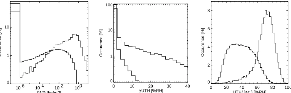
Figure 6shows in more detail how the cloud filter works on the database cases. It shows histograms of some important parameters, separately for the cases that were classified clear (thick line) and the cases that were classified cloudy (thin line). The leftmost plot shows histograms of IWP, confirming that the filter indeed removes most of the cases where a large amount of cloud ice is present. It shows also that the filter

15

is not perfect, as even the “clear” data contains still approximately 10% of cases with IWP exceeding 10 g/m2and 3% of cases with IWP exceeding 100 g/m2. On the other hand, some clear cases are erroneously marked as cloudy, approximately 36% of the “cloudy” dataset have IWP below 1 mg/m2.

The middle plot of Fig. 6 shows histograms of the cloud induced UTH error

20

(∆UTH=UTHtotalTb -UTH clear

Tb ). It confirms that the cloud filter drastically reduces this error. The cloud cases that remain in the “clear” class (i.e. those cases that are missed by the filter) lead to ∆UTH not larger than 14%RH, whereas otherwise ∆UTH can be up to 74%RH. (Note that the plot does not show data with ∆UTH exceeding 40%RH.)

The rightmost plot in Fig.6shows histograms of humidity itself (UTHJac). It confirms

25

that the cloudy cases indeed are associated with much higher UTH values than the clear cases. The maximum of the PDF is at approximately 70%RH. (Note that this relative humidity, as everywhere in this article, is over liquid water. If one uses relative

(15)

ACPD

7, 7509–7534, 2007

Full Screen / Esc

EGU

humidity over ice, the maximum of the PDF is at approximately 90%RH_i.)

The plot suggests yet another strategy how to deal with cloudy data, that is, to set all UTH values for cloudy scenes to 70%RH. For the midlatitude cloud dataset, this strategy leads to a mean UTH of 43.8%RH, which is indeed quite close to the true UTHclear_Tb . The problem with this strategy is that it can not be readily generalized to

5

global data, since we do not at present have statistics similar to the ones in Fig.6 for global data.

4 Conclusions

In this study a method for filtering high and strong ice clouds in AMSU-B microwave data was developed. The method combines two existing methods. One is thresholding

10

brightness temperatures from Channel 18 and the other one is thresholding brightness temperature differences between Channel 20 and 18. The method also takes into account the viewing geometry of the instrument, by using viewing angle dependent Channel 18 threshold values.

The robustness of the cloud filter was demonstrated in a case study of a

particu-15

larly strong ice cloud event over the UK, and by applying the filter to a database of midlatitude cloud cases.

These exercises show that the proposed cloud filter is well suited to filter out cloud contaminated data from AMSU-B. It should be possible to use the same technique also for other similar instruments.

20

The UTH retrieval method of Buehler and John (2005) was confirmed to be well suited for deriving a UTH climatology from AMSU-B Channel 18 data. Also, some new light was shed on the known limitations of this method. It was demonstrated, that the error that is referred to as regression noise in the earlier paper, is due to atmospheric profiles that are far from the mean of the profiles used to derive regression coefficients,

25

(16)

ACPD

7, 7509–7534, 2007

Full Screen / Esc

EGU

Furthermore, the impact of ice clouds on UTH area mean values derived from satel-lite microwave data was estimated. For the case study with a strong ice cloud, the scene averaged UTH value for the unfiltered data is 2%RH too wet, the cloud filtered UTH value is −3%RH too dry (both relative to the true scene averaged UTH value). For the general midlatitude cloud and clear-sky case database, the unfiltered mean

5

UTH is 0.8%RH too wet, the cloud filtered mean UTH is −2.4%RH too dry (both rel-ative to the true average UTH value). Both cloud- and cloud filtering bias are smaller in this case, as expected. These numbers are representative for general midlatitude conditions, since the case database was constructed to have realistic statistics. We conclude that, for midlatitudes, the best UTH retrieval strategy is to derive UTH with

10

and without cloud/surface filter, and use these as error bounds for the true value. The same strategy is likely to be also applicable to the tropics, but it is harder to prove this, since the radar-derived cases database is at present only available for mid-latitudes. However, a first look at global AMSU UTH data reveals that in the tropics the difference between total-sky and clear-sky UTH is also less than 3%RH. Thus, the

15

total-sky and clear-sky UTH values are useful error bounds for microwave data. For IR data they are also error bounds, but further apart, and hence less useful.

Besides the cloud issue, it was shown that the proposed filter also removes surface contaminated data, which can occur in certain areas in the winter season. The impact of surface contamination on UTH is comparable to the cloud impact, but slightly larger.

20

Also, the impact can be a low or high bias, depending on the surface conditions. In areas and seasons where surface contamination occurs the data should only be used with caution.

Acknowledgements. We acknowledge J. Miao for his work on the 2-D cloud filter. We thank

the UK MetOffice for providing us with the mesoscale model outputs. Also, we thank the ARTS 25

radiative transfer community. Many thanks to N. Courcoux for providing us with RTTOV sim-ulations. This study was partly funded by the German Federal Ministry of Education and Re-search (BMBF), within the AFO2000 project UTH-MOS, grant 07ATC04. It is a contribution to COST Action 723 “Data Exploitation and Modeling for the Upper Troposphere and Lower Stratosphere”.

(17)

ACPD

7, 7509–7534, 2007

Full Screen / Esc

EGU References

Adler, R. F., Mack, R. A., Prasad, N., Hakkarinen, I. M., and Yeh, H.-Y.: Aircraft Microwave Observations and Simulations of Deep Convection from 18 to 183 GHz. Part I: Observations, J. Atmos. Ocean Technol., 7, 377–391, 1990. 7512

Buehler, S. A. and John, V. O.: A Simple Method to Relate Microwave Radiances to Upper 5

Tropospheric Humidity, J. Geophys. Res., 110, D02110, doi:10.1029/2004JD005111, 2005.

7511,7522

Buehler, S. A., Eriksson, P., Kuhn, T., von Engeln, A., and Verdes, C.: ARTS, the Atmo-spheric Radiative Transfer Simulator, J. Quant. Spectrosc. Radiat. Transfer, 91, 65–93, doi:10.1016/j.jqsrt.2004.05.051, 2005. 7514,7516

10

Burns, B. A., Wu, X., and Diak, G. R.: Effects of Precipitation and Cloud Ice on Brightness Temperatures in AMSU Moisture Channels, IEEE T. Geosci. Remote, 35, 1429–1437, 1997.

7512

Chevallier, F.: Sampled databases of 60-level atmospheric profiles from the ECMWF analysis, Tech. rep., ECMWF, EUMETSAT SAF program research report no. 4, available at: http:

15

//www.metoffice.com/research/interproj/nwpsaf/rtm/profiles.pdf, 2001. 7514

Cullen, M. J. P.: The Unified Forecast/Climate Model, Meteorological Magazine, 122, 81–94, 1993. 7515

Emde, C., Buehler, S. A., Davis, C., Eriksson, P., Sreerekha, T. R., and Teichmann, C.: A Polarized Discrete Ordinate Scattering Model for Simulations of Limb and Nadir Long-20

wave Measurements in 1D/3D Spherical Atmospheres, J. Geophys. Res., 109, D24207, doi:10.1029/2004JD005140, 2004. 7516

English, S. J. and Hewison, T. J.: Fast generic millimeter-wave emissivity model, in: Proc. SPIE Vol. 3503, Microwave Remote Sensing of the Atmosphere and Environment, Tadahiro Hayasaka, Dong L. Wu, Ya-Qiu Jin, Jing-shan Jiang, edited by: Hayasaka, T., Wu, D. L., Jin, 25

Y.-Q., and Jiang, J.-S., 288–300, 1998. 7514,7516

Greenwald, T. J. and Christopher, S. A.: Effect of Cold Clouds on Satellite Measurements Near 183 GHz, J. Geophys. Res., 107, 4170, doi:10.1029/2000JD0002580, 2002. 7512, 7514,

7517,7519

Hong, G., Heygster, G., Miao, J., and Kunzi, K.: Detection of tropical deep convective 30

clouds from AMSU-B water vapor channels measurements, J. Geophys. Res., 110, D05205, doi:10.1029/2004JD004949, 2005. 7512

(18)

ACPD

7, 7509–7534, 2007

Full Screen / Esc

EGU Jakob, C.: Ice clouds in numerical weather prediction models: Progress, problems, and

prospects, in: Cirrus, edited by: Lynch, D. K., Sassen, K., Starr, D. O., and Stephens, G., 327–345, Oxford University Press, New York, 2002. 7517

McFarquhar, G. M. and Heymsfield, A. J.: Parameterization of Tropical Cirrus Ice Crystal Size Distribution and Implications for Radiative Transfer: Results from CEPEX, J. Atmos. Sci., 54, 5

2187–2200, 1997. 7516

Pruppacher, H. R. and Klett, J. D.: Microphysics of Clouds and Precipitation, Kluwer Academic Publishers, The Netherlands, reprinted with corrections 2000, 1997.7517

Quante, M. and Starr, D.: Dynamical processes in cirrus clouds: A Review of Observational Results, in: Cirrus, edited by: Lynch, D. K., Sassen, K., Starr, D. O., and Stephens, G., 10

346–374, Oxford University Press, New York, 2002. 7517

Saunders, R., Matricardi, M., and Brunel, P.: An improved fast radiative transfer model for assimilation of satellite radiance observations, Quart. J. Roy. Meteorol. Soc., 125, 1407– 1425, 1999. 7514

Saunders, R. W., Hewison, T. J., Stringer, S. J., and Atkinson, N. C.: The Radiometric Charac-15

terization of AMSU-B, IEEE T. Microw. Theory, 43, 760–771, 1995. 7511

Soden, B. J. and Bretherton, F. P.: Interpretation of TOVS water vapor radiances in terms of layer-average relative humidities: Method and climatology for the upper, middle, and lower troposphere, J. Geophys. Res., 101, 9333–9344, doi:10.1029/96JD00280, 1996.7511,7519

Soden, B. J. and Lanzante, J. R.: An Assessment of Satellite and Radiosonde Climatologies of 20

Upper-Tropospheric Water Vapor, J. Climate, 9, 1235–1250, 1996. 7518

Sreerekha, T. R.: Impact of clouds on microwave remote sensing, Ph.D. thesis, University of Bremen, 2005. 7517

Wu, D. L., Jiang, J. H., and Davis, C.: EOS MLS Cloud Ice Measurements and Cloudy-Sky Radiative Transfer Model, IEEE T. Geosci. Remote, 44, 1156–1165, 2006. 7516

(19)

ACPD

7, 7509–7534, 2007

Full Screen / Esc

EGU

Table 1. Viewing angle (θ in degrees from nadir) dependent thresholds for Channel 18

bright-ness temperatures (in K).

θ T_B18 θ T_B18 θ T_B18 θ T_B18 θ T_B18 0.55 240.1 10.45 239.8 20.35 239.2 30.25 238.2 40.15 236.4 1.65 240.1 11.55 239.8 21.45 239.2 31.35 238.0 41.25 236.1 2.75 240.1 12.65 239.7 22.55 239.1 32.45 237.8 42.35 235.8 3.85 240.1 13.75 239.7 23.65 239.0 33.55 237.6 43.45 235.5 4.95 240.1 14.85 239.6 24.75 238.8 34.65 237.4 44.55 235.2 6.05 240.1 15.95 239.6 25.85 238.7 35.75 237.2 45.65 234.9 7.15 240.1 17.05 239.5 26.95 238.6 36.85 237.0 46.75 234.4 8.25 239.9 18.15 239.4 28.05 238.5 37.95 236.7 47.85 233.9 9.35 239.9 19.25 239.3 29.15 238.3 39.05 236.6 48.95 233.3

(20)

ACPD

7, 7509–7534, 2007

Full Screen / Esc

EGU

Table 2. Mean and median UTH in the scene for different kinds of data. All values are in %RH.

Data mean median std min max

UTH_Jac 58.04 60.36 11.99 14.66 81.13

UTHclear_Tb 57.16 59.78 10.86 20.56 73.04

UTHtotal_Tb 59.12 60.60 12.86 20.56 108.30

(21)

ACPD

7, 7509–7534, 2007

Full Screen / Esc

EGU

Table 3. Mean and median UTH in the cloud database for different kinds of data. All values are

in %RH.

Data mean median std min max

UTH_Jac 42.76 41.54 17.48 0.81 96.58

UTHclear_Tb 43.40 42.80 15.12 5.30 99.73

UTHtotal_Tb 44.17 43.19 16.03 5.30 99.99

(22)

ACPD

7, 7509–7534, 2007

Full Screen / Esc

Printer-friendly Version Interactive Discussion EGU −60 −40 −20 0 20 40 60 Tb(20) − Tb(18) [K] 220 240 260 280 Tb(18) NOAA−16(Nadir),Lat 45−50 0.0001 0.0001 0.001 0.001 0.001 0.01 0.01 0.1 0.5 −60 −40 −20 0 20 40 60 220 240 260 280 Tb(18) ECMWF(RTTOV),Lat 45−50 0.0001_0.001 0.01 0.1 −60 −40 −20 0 20 40 60 220 240 260 280 Tb(18) NOAA−16(Off−nadir),Lat 45−50 0.0001 0.0001 0.0001 0.001 0.001 0.001 0.01 0.01 0.1 0.5 0.0001 0.0010 0.0100 0.1000 0.5000 1.0000

Fig. 1. Left plot: combined histogram of the measured difference between AMSU-B

Chan-nel 20 and 18 brightness temperatures (y-axis) and ChanChan-nel 18 brightness temperature (x-axis). Fields of view (FOVs) used were the five innermost FOVs on both sides from nadir, with FOV numbers 41–50. Middle plot: RTTOV simulation of clear-sky brightness temperatures from ECMWF data. The data are for January 2004, near nadir viewing geometry, and a 45–50 latitude band. Right plot: the same as on the left, but for off-nadir looking measurements. FOVs used were the five outermost FOVs on both edges of the scanline, with FOV numbers 1–5 and 86–90.

(23)

ACPD

7, 7509–7534, 2007

Full Screen / Esc

Printer-friendly Version Interactive Discussion EGU Jacobian UTH 340˚ 340˚ 350˚ 350˚ 0˚ 0˚ 10˚ 10˚ 50˚ 50˚ 60˚ 60˚ 0 10 20 30 40 50 60 70 80 90 100 %RH

Clear−sky UTH − Jacobian UTH

340˚ 340˚ 350˚ 350˚ 0˚ 0˚ 10˚ 10˚ 50˚ 50˚ 60˚ 60˚ −22 −15 −10 −5 0 5 10 %RH 0 20 40 60 80 100 Jacobian UTH [%RH] 0 20 40 60 80 100 Clear-sky UTH [%RH]

Fig. 2. A comparison between clear-sky simulated brightness temperatures converted to UTH_Tb and UTH_Jac. Left: Model UTH_Jac; middle: UTH_Tb-UTH_Jac; right: Scatter plot of UTH_Tb versus UTH_Jac. Relative humidity here, as everywhere in the paper, is defined over liquid water.

(24)

ACPD

7, 7509–7534, 2007

Full Screen / Esc

EGU

Ice Water Path

340˚ 340˚ 350˚ 350˚ 0˚ 0˚ 10˚ 10˚ 50˚ 50˚ 60˚ 60˚ 0.00.1 0.3 0.5 1.5 2.5 3.5 kg/m2 Measured Tbs 340˚ 340˚ 350˚ 350˚ 0˚ 0˚ 10˚ 10˚ 50˚ 50˚ 60˚ 60˚ 230 233 236 239 242 245 248 251 254 257 K

Total−sky UTH − Clear−sky UTH

340˚ 340˚ 350˚ 350˚ 0˚ 0˚ 10˚ 10˚ 50˚ 50˚ 60˚ 60˚ 0 2 8 14 20 30 50 %RH

Cloud Top Altitude

340˚ 340˚ 350˚ 350˚ 0˚ 0˚ 10˚ 10˚ 50˚ 50˚ 60˚ 60˚ 950 6500 7000 7500 8000 8500 9000 9500 10000 10500 11000 11500 m Simulated Tbs 340˚ 340˚ 350˚ 350˚ 0˚ 0˚ 10˚ 10˚ 50˚ 50˚ 60˚ 60˚ 230 233 236 239 242 245 248 251 254 257 K

Total−sky UTH − Clear−sky, with cloud filter

340˚ 340˚ 350˚ 350˚ 0˚ 0˚ 10˚ 10˚ 50˚ 50˚ 60˚ 60˚ 0 2 8 14 20 30 50 %RH

Fig. 3. Left column, top plot: mesoscale NWP model IWP field. Left column, bottom plot: cloud

top altitude in meters, defined as the highest altitude where the ice water content is larger than 10−5_kg/m3

. Middle column, top plot: Measured AMSU-B channel 18 radiances. Middle column, bottom plot: ARTS RT model simulation, based on model fields. Right column, top plot: UTH difference between the full simulation and a simulation with cloud ice amount set to zero. Right column, bottom plot: The same as on the top, but with applied cloud filter.

(25)

ACPD

7, 7509–7534, 2007

Full Screen / Esc

Printer-friendly Version Interactive Discussion EGU NOAA−16, summer, 2001 0˚ 0˚ 40˚ 40˚ 80˚ 80˚ 120˚ 120˚ 160˚ 160˚ 200˚ 200˚ 240˚ 240˚ 280˚ 280˚ 320˚ 320˚ 0˚ 0˚ −40˚ −40˚ 0˚ 0˚ 40˚ 40˚ 0˚ 0˚ 40˚ 40˚ 80˚ 80˚ 120˚ 120˚ 160˚ 160˚ 200˚ 200˚ 240˚ 240˚ 280˚ 280˚ 320˚ 320˚ 0˚ 0˚ −40˚ −40˚ 0˚ 0˚ 40˚ 40˚ 5 10 15 20 25 35 45 55 60 65 70 UTH [%RH]

Total − Clear Sky, NOAA−16, summer, 2001

0˚ 0˚ 40˚ 40˚ 80˚ 80˚ 120˚ 120˚ 160˚ 160˚ 200˚ 200˚ 240˚ 240˚ 280˚ 280˚ 320˚ 320˚ 0˚ 0˚ −40˚ −40˚ 0˚ 0˚ 40˚ 40˚ 0˚ 0˚ 40˚ 40˚ 80˚ 80˚ 120˚ 120˚ 160˚ 160˚ 200˚ 200˚ 240˚ 240˚ 280˚ 280˚ 320˚ 320˚ 0˚ 0˚ −40˚ −40˚ 0˚ 0˚ 40˚ 40˚ −8 −5 −4 −3 −2 −1 1 2 3 4 5 11 UTH [%RH]

Fig. 4. Top: Seasonal UTH climatology derived from 183.31±1.00 GHz microwave data from

the NOAA 16 satellite between June 2001 and August 2001. Bottom: Difference between UTH derived from all available data and UTH derived from data which passed the cloud filter described in the previous section. Minimum, maximum, and mean of the UTH difference in the lower plot are −3.9, 3.9 and 0.6±0.6%RH respectively.

(26)

ACPD

7, 7509–7534, 2007

Full Screen / Esc

Printer-friendly Version Interactive Discussion EGU NOAA−16, winter, 2001 0˚ 0˚ 40˚ 40˚ 80˚ 80˚ 120˚ 120˚ 160˚ 160˚ 200˚ 200˚ 240˚ 240˚ 280˚ 280˚ 320˚ 320˚ 0˚ 0˚ −40˚ −40˚ 0˚ 0˚ 40˚ 40˚ 0˚ 0˚ 40˚ 40˚ 80˚ 80˚ 120˚ 120˚ 160˚ 160˚ 200˚ 200˚ 240˚ 240˚ 280˚ 280˚ 320˚ 320˚ 0˚ 0˚ −40˚ −40˚ 0˚ 0˚ 40˚ 40˚ 5 10 15 20 25 35 45 55 60 65 70 UTH [%RH]

Total − Clear Sky, NOAA−16, winter, 2001

0˚ 0˚ 40˚ 40˚ 80˚ 80˚ 120˚ 120˚ 160˚ 160˚ 200˚ 200˚ 240˚ 240˚ 280˚ 280˚ 320˚ 320˚ 0˚ 0˚ −40˚ −40˚ 0˚ 0˚ 40˚ 40˚ 0˚ 0˚ 40˚ 40˚ 80˚ 80˚ 120˚ 120˚ 160˚ 160˚ 200˚ 200˚ 240˚ 240˚ 280˚ 280˚ 320˚ 320˚ 0˚ 0˚ −40˚ −40˚ 0˚ 0˚ 40˚ 40˚ −8 −5 −4 −3 −2 −1 1 2 3 4 5 11 UTH [%RH]

Fig. 5. Cloud and surface effects on AMSU-B data. This is the same as Fig.4, but the data used are from December 2001 to February 2002. Minimum, maximum and mean of the UTH difference in the lower plot are −7.3, 10.7 and 0.6±1.0%RH respectively.

(27)

ACPD

7, 7509–7534, 2007

Full Screen / Esc

Printer-friendly Version Interactive Discussion EGU 10-6 10-4 10-2 100 IWP [kg/m2] 0 1 10 Occurence [%] 0 10 20 30 40 ∆UTH [%RH] 0 1 10 100 Occurence [%] 0 20 40 60 80 100 UTH(Jac.) [%RH] 0 2 4 6 8 Occurence [%]

Fig. 6. Histograms of some key parameters for cases that were classified clear (thick line)

and cases that were classified cloudy (thin line). Left: IWP; middle: ∆UTH; right: UTHJac. The binsize of UTH_Jacand ∆UTH are 2%RH. The binsize of IWP follows the logarithmic scale of the x-axis. Note that the leftmost bin of the IWP histogram contains all data between 0 and 0.001 g/m2. The “clear” class contains approximately 150 000 cases, the “cloudy” class approximately 20 000 cases.