Study of electromagnetic diffraction by curved strip gratings by use of the C-method

HAL Id: hal-00255748

https://hal.archives-ouvertes.fr/hal-00255748

Submitted on 22 Apr 2021

HAL is a multi-disciplinary open access

archive for the deposit and dissemination of

sci-entific research documents, whether they are

pub-lished or not. The documents may come from

teaching and research institutions in France or

abroad, or from public or private research centers.

L’archive ouverte pluridisciplinaire HAL, est

destinée au dépôt et à la diffusion de documents

scientifiques de niveau recherche, publiés ou non,

émanant des établissements d’enseignement et de

recherche français ou étrangers, des laboratoires

publics ou privés.

Distributed under a Creative Commons Attribution| 4.0 International License

Study of electromagnetic diffraction by curved strip

gratings by use of the C-method

B. Guizal, G. Granet

To cite this version:

B. Guizal, G. Granet. Study of electromagnetic diffraction by curved strip gratings by use of the

C-method. Journal of the Optical Society of America. A Optics, Image Science, and Vision, Optical

Society of America, 2007, 24 (3), pp.669-674. �10.1364/JOSAA.24.000669�. �hal-00255748�

Study of electromagnetic diffraction by curved

strip gratings by use of the C-method

B. Guizal

Départment d’Optique P. M. Duffieux, Institut Franche-Comté Electronique, Mécanique, Thermique et Optique–Sciences et Technologies, UMR 6174 du CNRS, 16, Route de Gray, 25030 Besanon Cedex, France

G. Granet

Laboratoire des Sciences et Matériaux pour l’Electronique, et d’Automatique, UMR CNRS 6602, Université Blaise Pascal Les Cézeaux, 24 avenue des Landais, 63177 Aubière Cedex, France

The C-method is one of the most efficient and versatile methods designed for diffraction gratings. Its strength lies in the use of a coordinate system in which the surface of the grating coincides with a coordinate surface. The result is a great simplification in writing the boundary conditions. We exploit this simplification to treat the problem of diffraction from curved strip gratings, and we use the combined boundary conditions method that has _{been introduced for planar strip gratings and proved to be very efficient.}

1. INTRODUCTION

Diffraction from strip gratings is a well-known problem that has been extensively studied in the past. These structures have been used to model photolithographic masks as well as optical or microwave filters or frequency selective surfaces. Although some rigorous methods do ex-ist that can model more realex-istic situations, i.e., strips with finite conductivity and non-null thickness, the per-fect (in the sense perper-fectly conducting and infinitely thin) strip grating approach remains interesting and can even be competitive when one is dealing with highly conduct-ing materials with a sufficiently small thickness com-pared to the wavelength, as can be the case of noble met-als in the terahertz domain. One of the most versatile and efficient methods designed for perfectly conducting strip gratings is the combined boundary conditions method (CBCM).1The key feature of this differential approach is that it combines the continuity equations of the electric and the magnetic fields in a unified equation that holds over one full period. Thus all the continuity equations can be projected on the Fourier basis permitting simple calcu-lations. This method has been applied to strip gratings1 as well as bulk ones2 and adapted successfully to aperi-odic strips gratings3and to circular geometry.4

On the other hand, the C-method5is one of the most el-egant and efficient methods introduced for surface relief diffraction gratings. Its strength lies in the use of a coor-dinate system in which the surface of the grating coin-cides with a coordinate surface. The result is a great sim-plification in writing the boundary conditions. Since its introduction in 1982, this approach has been generalized to multilayered diffraction gratings6 and to crossed gratings.7 In this work, we apply the C-method to the study of curved diffraction gratings.

In Sections 2 and 3 the key steps of the C-method and the CBCM are outlined in order to give some self-consistency to the paper. Sections 4 and 5 are dedicated to the writing of the boundary conditions through the con-cept of the CBCM. Finally, some numerical examples are given to illustrate the effectiveness of this new approach.

2. THEORY

The structure under study is depicted in Fig. 1. It consists of a one-dimensional grating separating two dielectric ho-mogeneous media and over which is deposited an infi-nitely thin perfectly conducting grating of the same shape and period. The surface of the grating is invariant along the z direction, and we assume that its cross section (i.e., the shape of the grating) can be described by a function,

a共x兲. It is known from previous work5that it is possible to introduce a new coordinate system such that the surface of the grating coincides with a coordinate surface. Such a system, called the translation coordinate system, can be defined from the Cartesian coordinates as follows:

x1_{= x,}

x2_{= u = y − a共x兲,}

x3_{= z. 共1兲}

In the new coordinate system共x,u,z兲, the surface of the grating is exactly that of equation u = 0. This makes the boundary conditions much simpler to write, as will be re-called later. In this coordinate transformation, the metric tensor writes

共glm_{兲 =}

冤

g11 g12 g13 g21 g22 g23 g31 g32 g33

冥

=

冤

1 − a˙ 0 − a˙ 1 + a˙2 ₀ 0 0 1

冥

, a˙ =da共x兲 dx . 共2兲

One can remark that the matrix共glm_{兲 is not diagonal,}

which means that the new coordinate system is nonor-thogonal. Thus it seems natural to use Maxwell’s equa-tions under their tensor form that has been derived from relativistic electrodynamics. In this work, we will use Maxwell’s equations under the covariant form introduced by Post.8

Working with linear, homogeneous, and isotropic media and assuming that time dependence is handled by the term exp共i␻t兲, the complex amplitudes Enand Hn of the

covariant components of the electric and the magnetic fields are linked by the following Maxwell’s equations:

␰lmn_⳵

mEn= − i␻␮0

冑

gglmHm,

␰lmn⳵_mHn= i␻␧0␯2

冑

gglmEm,

1 艋 l,m,n 艋 3, g = det共glm兲. 共3兲

␧0and ␮0 are the dielectric permittivity and the

mag-netic permeability of vacuum, respectively; ␯ is the refrac-tive index of the medium; and ⳵mdenotes the derivation

operator with respect to variable xm_{. ␰}lmn _{is the Levi–}

Civita indicator defined by

␰lmn₌

冦

1 if共lmn兲 is an even permutation of 共123兲 − 1 if共lmn兲 is an odd permutation of 共123兲 0 otherwise

冧

. 共4兲 If we substitute the metric tensor共glm_{兲 from Eq. (2) into}

Eqs. (3), and keeping in mind that the problem is z invari-ant (i.e., ⳵3⬅0), we obtain

⳵_2E3= − i␻␮0共H1− a˙H2兲,

− ⳵1E3= − i␻␮0共− a˙H1+共1 + a˙2兲H2兲,

⳵_{1E2− ⳵2E1= − i␻␮0H3,} 共5兲 ⳵_{2H3= i␻␧0␯}2共E_{1− a˙E2}兲,

− ⳵1H3= i␻␧0␯2共− a˙E1+共1 + a˙2兲E2兲,

⳵₁H2− ⳵2H1= i␻␧0␯2E3. 共6兲

From these equations, it can be shown5 that the two types of polarization (TE and TM) are described by the same set of differential equations:

⳵_uF共x,u兲 = d共x兲⳵xF共x,u兲 − ikc共x兲G共x,u兲,

⳵_uG共x,u兲 = −

i k

⳵_x关c共x兲⳵_xF共x,u兲兴 − ikF共x,u兲

+ ⳵x关d共x兲G共x,u兲兴, 共7兲

where c共x兲=1/共1+a˙2_{兲, d共x兲=a˙/共1+a˙}2_{兲, and k = k} 0␯

= ␻

冑

⑀0␮0␯. The TE case corresponds to F = Ez and G

= ZHx whereas the TM case corresponds to F = ZHz and

G = −Exwith Z =

冑

共␮0/ ⑀0兲/␯=Z0/ ␯.

Due to the x periodicity, c共x兲 and d共x兲 can be expanded in their Fourier series whereas F共x,u兲 and G共x,u兲 are ex-panded in generalized Fourier series:

c共x兲 =

兺

m cmexp共− im2␲x/d兲, d共x兲 =

兺

m dmexp共 − im2␲x/d兲,

F共x,u兲 = exp共− i␣0x兲

兺

m

Fm共u兲exp共− im2␲x/d兲,

G共x,u兲 = exp共− i␣0x兲

兺

m

Gm共u兲exp共− im2␲x/d兲. 共8兲

Here ␣0is a real number (often called the quasiperiodicity

factor) that stands for the x component of the incident wave vector. Introducing these expressions in Eqs. (7) and projecting on the Fourier basis, gives

d du

冋

Fm Gm

册

= − i

冤

关兩d兩兴␣ k关兩c兩兴 k −1 k␣关兩c兩兴␣ ␣关兩d兩兴

冥

冋

Fm Gm

册

, 共9兲 ␣ = diag共␣˙0+ m2␲ / d兲, 关兩c兩兴=共1+关兩a˙兩兴⫻关兩a˙兩兴兲−1, 关兩d兩兴=关兩c兩兴

⫻关兩a˙兩兴, and 关兩a˙兩兴mn is the 共m−n兲th Fourier coefficient in

the development of a˙共x兲. It is worth noting that the cor-rect rules of Fourier factorization9have been used. Equa-tion (9) can be written under the more concise form

dF

du= AF共u兲, F =

冋

Fm共u兲

Gm共u兲

册

. 共10兲 Ais the matrix appearing in Eq. (9). At this stage we truncate the differential system by keeping only the or-ders such that −M 艋 m 艋 M (M will be called the trunca-tion order). Then, assuming a u dependence in exponen-tial form, the above differential system can be transformed into an eigenvalue problem:

rnFn= AFn, 共11兲

where rnis an eigenvalue of A, and Fnis its

correspond-ing eigenvector. At this stage and to distcorrespond-inguish between propagating and evanescent waves and between those propagating toward the grating and those traveling to

finity, the eigenvalues are sorted according to their real and imaginary parts.5Finally, the fields corresponding to our diffraction problem can be written

medium 1: F1共x,u兲 =

兺

m=−M M

再

F_m0incexp共r10u兲 +

兺

n=1 2M+1 RnFmn diff_exp共r 1nu兲

冎

⫻exp共− i␣mx兲, G1共x,u兲 =

兺

m=−M M

再

G_m0incexp共r10u兲 +

兺

n=1 2M+1 RnGmn diff

⫻exp共r1nu兲

冎

exp共− i␣mx兲, 共12兲

medium 2: F2共x,u兲 =

兺

m=−M M

再

兺

n=1 2M+1 TnFmn tr _exp共r 2nu兲

冎

exp共− i␣mx兲, G2共x,u兲 =

兺

m=−M M

再

兺

n=1 2M+1

TnGmntr exp共r2nu兲

冎

exp共− i␣mx兲,

共13兲 where r10is the eigenvalue corresponding to the incident

plane wave while r1/2n corresponds to the reflected

共propagating+evanescent兲 or transmitted 共propagating + evanescent兲 waves in mediums 1 and 2, respectively. Rn

and Tnare the reflection and the transmission amplitudes

to be determined via the boundary conditions. As men-tioned in Section 1, we will use the CBCM, and therefore it is useful to give an idea about the principle of this method.

3. PRINCIPLE OF THE COMBINED

BOUNDARY CONDITIONS METHOD

In this section, we briefly recall the principle of the CBCM for flat strip gratings. The interested reader can find de-tailed developments in Refs. 1, 2, and 10. The situation is that of Fig. 1 with a null height. The boundary conditions at the interface y = 0 impose that

• the tangential electric field must be continuous over a whole period;

• the tangential electric field must be null over the strips; and

• the magnetic field must be continuous over the complementary of the strips.

The main idea behind the CBCM is to combine the last two conditions in a single one that is valid over a whole period. The benefit is that one can use the orthonormal Fourier basis关exp共−i␣mx兲兴 as projection one.

In the TE polarization case, these conditions write

E1z共x,y兲 = E2z共x,y兲 for 0 ⬍ x ⬍ D, E1z共x,y兲 = E2z共x,y兲 = 0 for 0 ⬍ x ⬍ w,

H1x共x,y兲 = H2x共x,y兲 for w ⬍ x ⬍ D, 共14兲

and can be recast, as mentioned above, to the following set of two relations:

∀0 ⬍ x

⬍ D

再

E1z共x,y兲 = E2z共x,y兲

␹共x兲E2z共x,y兲 + ␶关1 − ␹共x兲兴关H2x共x,y兲 − H1x共x,y兲兴 = 0,

冎

共15兲 where ␹共x兲 is the characteristic function of the strips, i.e., ␹共x兲=1 over the strips and zero elsewhere. ␶ is a numeri-cal parameter introduced for dimensional and numerinumeri-cal purpose: As we mix boundary conditions involving the electric and the magnetic fields, that are of different mag-nitudes, a problem of bad numerical conditioning of the matrices can arise. This is avoided by introducing the pa-rameter ␶ that can be adjusted in such a way that the two terms constituting the mixed equation are of the same scale. In principle the second equation, in Eq. (15) is valid whatever the value of ␶ (see Ref. 1, for example).

In the TM polarization case, the boundary conditions write

E1x共x,y兲 = E2x共x,y兲 for 0 ⬍ x ⬍ D, E1x共x,y兲 = E2x共x,y兲 = 0 for 0 ⬍ x ⬍ w,

H1z共x,y兲 = H2z共x,y兲 for w ⬍ x ⬍ D, 共16兲

and can be recast to ∀0 ⬍ x

⬍ D

再

E1x共x,y兲 = E2x共x,y兲

␹共x兲E2x共x,y兲 + ␶关1 − ␹共x兲兴关H2z共x,y兲 − H1z共x,y兲兴 = 0

冎

. 共17兲 Thus writing the boundary conditions through the con-cept of the CBCM consists of using Eqs. (15) in the TE case and Eqs. (17) in the TM case. Now we are going to apply this principle to the curved strip grating described in Section 1. For that purpose it is convenient to separate the two types of polarization.

4. TE POLARIZATION

In this case, and by use of the CBCM, the boundary con-ditions on the surface y = a共x兲 are expressed through Eqs. (15), which give, in the translation coordinates system, on the surface that corresponds to u = 0:

∀0 ⬍ x ⬍ D

冦

F1共x,u = 0兲 = F2共x,u = 0兲 ␹共x兲F2共x,0兲 + ␶关1 − ␹共x兲兴

冋

1 Z2 G2共x,0兲 − 1 Z1 G1共x,0兲

册

= 0.

冧

共18兲

Expanding the characteristic function in Fourier series and projecting the above equations on the exponential ba-sis gives, in vector notation,

Finc+ Fdiff_{R = F}tr_T,

关兩␹兩兴Ftr_{T +} ␶

Z0

关I − 关兩␹兩兴兴兵␯1GtrT − ␯2共Ginc+ GdiffR兲其 = 0. 共19兲

I stands for the identity matrix and关兩␹兩兴 is the toeplitz

matrix whose 共m,n兲th elements are the Fourier coeffi-cients ␹m−n. The rest of the work is rather mechanical.

The linear system of Eqs. (19) is solved for R and T from which the fields can be calculated everywhere.

5. TM POLARIZATION

In this second case, the boundary conditions on the sur-face defined by u = 0, in the translation coordinates sys-tem, write ∀0 ⬍ x ⬍ D

再

G1共x,u = 0兲 = G2共x,u = 0兲. ␹共x兲G2共x,0兲 + ␶关1 − ␹共x兲兴关F2共x,0兲 − F1共x,0兲兴 = 0

冎

. 共20兲 By expanding the characteristic function in Fourier se-ries and projecting the above equations on the exponen-tial basis, we obtain in vector notations

Ginc_{+ G}diff_{R = G}tr_T,

关兩␹兩兴Gtr_{T +} ␶

Z0

关I − 关兩␹兩兴兴兵␯1FtrT − ␯2共Finc+ FdiffR兲其 = 0. 共21兲

As in the TE case, the linear system of Eqs. (21) is solved for R and T from which the fields can be calculated everywhere.

6. EFFICIENCIES

Finally, application of Poyntings theorem, written in the translation coordinates, enables us to calculate the power carried by the nth diffracted and transmitted waves. Dif-fraction efficiencies are then defined as the ratio of these powers to that carried by the incident wave5:

ern=兩Rn兩2 Re

冉

兺

m=−M M F_mndiffG_mndiff

冊

Re

冉

兺

m=−M M F_m0incG_m0inc

冊

, etn= ␯2 ␯₁兩Tn兩 2 Re

冉

兺

m=−M M F_mntr G_mntr

冊

Re

冉

兺

m=−M M F_m0incG_m0inc

冊

. 共22兲

7. RESULTS

In this section, we provide some numerical results to il-lustrate the effectiveness of the presented method. Let us first emphasize that the convergence of the method has been checked against usual criteria such as energy con-servation (up to 10−9_{) and reciprocity laws.}

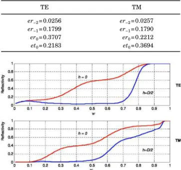
As a first example we consider a sinusoidal profile de-scribed by the function a共x兲=h/2 cos共2␲x/D兲. We begin by setting h = 0, and verify that we recover the results ob-tained from the classical CBCM in the case of planar structures as published in Ref. 10. The period is such that ␭ = 0.7D, the gap between the slits is w = D / 2, the inci-dence angle is ␪ = 26° while the surrounding medium is vacuum. The truncation order has been taken equal to 256 and ␶ has been set to 0.01i. In Table 1 we give our computed reflected and transmitted efficiencies for both cases of polarization with h = 0. These results match those of Ref. 10.

We now set the height of the grating to D / 2 (all the other parameters being unchanged) and observe the re-flectivity (sum of all the reflected efficiencies) of the struc-ture versus the parameter w. Figure 2 demonstrates the change in reflectivity when the planar strips are bent. The case of TE polarization is remarkable because of the quick variation in reflectivity that appears near w = 0.75D, which approximately corresponds to the wave-length. This could be explained by the formation of a cav-ity corresponding to the lower part of the cosine function. In the second example, and for the purpose of valida-tion, we compare our results to those obtained by an inte-gral approach.11The profile is trapezoidal as depicted in Fig. 3 and the metal is deposited along the lateral sides of the trapezium. As can be seen from Fig. 4, where the re-flected efficiencies are drawn as functions of the param-eter D / ␭, our results coincide exactly with those of Ref. 11. Furthermore, we verified that by setting the strips on

Table 1. Computed Diffraction Efficiencies for h = 0

TE TM

er−2= 0.0256 er−2= 0.0257

er−1= 0.1799 er−1= 0.1790

er₀= 0.3707 er₀= 0.2212 et0= 0.2183 et0= 0.3694

Fig. 2. (Color online) Reflectivity as a function of the width w of the strips.

one horizontal part of the trapezium we recover the re-sults computed by use of the classical planar CBCM.

As an application, we consider a metallic (silver) sinu-soidal grating that can support a surface plasmon. Let us imagine now an academic experience in which this struc-ture is partially covered by a strip grating and illumi-nated by a monochromatic plane wave under TM polar-ization. In this example, we neglect the dispersion and set ⑀sil= −17.6+ 0.67j. Figure 5 shows the evolution of the

cal-culated reflectivity versus the wavelength for various widths w of the strips. We notice that as the width of the strips is increased, the dip in reflection that is character-istic of the excitation of a surface plasmon is shifted to-ward the lower part of the spectrum and at the same time becomes more and more sharp. This behavior is due to the fact that the presence of the strips affects the dispersion relation of the original silver grating that is responsible for the shift of the plasmon resonance. The fineness of the dips can be easily understood if one keeps in mind that their width is directly related to the losses in the metal (silver). As the lossy metal is covered by the perfectly con-ducting strips that are lossless, the amount of losses is re-duced and thus the resonances are sharper. A more de-tailed study of this interesting phenomenon is in progress that introduces the real dispersion of silver in the model and computes the map of the fields around the strips.

8. CONCLUSION

A method has been presented that combines two of the most efficient known methods in the field of diffraction grating theories. We showed that this new approach is general in the sense that it allows the study of curved strip gratings of various shapes with a rather low compu-tational effort. Furthermore, numerical examples were given with tabulated values that can be useful for those who want to check their codes.

Finally, let us emphasize that the method can be easily adapted for the study of multilayered strip structures and can be extended, without great difficulty, to crossed curved gratings.

B. Guizal’s e-mail address is bguizal@univ-fcomte.fr.

REFERENCES

1. F. Montiel and M. Nevière, “Electromagnetic study of the diffraction of light by a mask used in photolithography,” Opt. Commun. 101, 151–156 (1993).

2. F. Montiel and M. Nevière, “Perfectly conducting gratings: a new approach using infinitely thin strips,” Opt. Commun.

144, 82–88 (1997).

3. B. Guizal and D. Felbacq, “Electromagnetic beam diffraction by a finite strip grating,” Opt. Commun. 165, 1–6 (1999).

4. B. Guizal and D. Flebacq, “Numerical computation of the scattering matrix of an electromagnetic resonator,” Phys. Rev. E 66, 026602 (2002).

5. J. Chandezon, M. T. Dupuis, G. Cornet, and D. Maystre, “Multicoated gratings: a differential formalism applicable in the entire optical region,” J. Opt. Soc. Am. 72, 839–846 (1982).

6. G. Granet, J. P. Plumey, and J. Chandezon, “Scattering by a periodically corrugated dielectric layer with non-identical faces,” Pure Appl. Opt. 4, 1–5 (1995).

7. G. Granet, “Analysis of diffraction by crossed gratings Fig. 3. (Color online) Schematic view of the trapezoidal grating

used in example 2. D =兺i=1,4ai with a2= a4= D / 3 and a1= a3

= D / 6 = h tan共␲/ 6兲. The angle of incidence is set to 0.1°.

Fig. 4. (Color online) Evolution of the different reflected effi-ciencies er_{共−1,0,1兲}versus D / ␭.

Fig. 5. (Color online) Reflectivity versus the wavelength for a metallic sinusoidal grating covered with strips of various widths. h = 0.05␮m, D = 0.6␮m,⑀_sil= −17.6+ 0.67j.

using a non-orthogonal coordinate system,” Pure Appl. Opt.

4, 777–793 (1995).

8. E. J. Post, Formal Structure of Electromagnetics (North Holland, 1962).

9. L. Li and J. Chandezon, “Improvement of the coordinate transformation method for surface-relief gratings with sharp edges,” J. Opt. Soc. Am. A 13, 2247–2255 (1996).

10. G. Granet and B. Guizal, “Analysis of strip gratings using a parametric modal method by Fourier expansions,” Opt. Commun. 255, 1–11 (2005).

11. R. C. Hall, R. Mittra, and K. M. Mitzner, “Scattering from finite thickness resistive strip gratings,” IEEE Trans. Antennas Propag. 36, 504–510 (1988).