HAL Id: hal-00758187
https://hal.inria.fr/hal-00758187
Submitted on 29 Nov 2012
HAL is a multi-disciplinary open access
archive for the deposit and dissemination of
sci-entific research documents, whether they are
pub-lished or not. The documents may come from
teaching and research institutions in France or
abroad, or from public or private research centers.
L’archive ouverte pluridisciplinaire HAL, est
destinée au dépôt et à la diffusion de documents
scientifiques de niveau recherche, publiés ou non,
émanant des établissements d’enseignement et de
recherche français ou étrangers, des laboratoires
publics ou privés.
A benchmark for cooperative coevolution
Alberto Tonda, Evelyne Lutton, Giovanni Squillero
To cite this version:
Alberto Tonda, Evelyne Lutton, Giovanni Squillero.
A benchmark for cooperative coevolution.
(will be inserted by the editor)
A Benchmark for Cooperative Coevolution
Alberto Tonda and Evelyne Lutton and Giovanni Squillerothe date of receipt and acceptance should be inserted later
Abstract Cooperative co-evolution algorithms (CCEA) are a thriving sub-field of evolutionary computation. This class of algorithms makes it possible to exploit more efficiently the artificial Darwinist scheme, as soon as an optimisation problem can be turned into a co-evolution of interdependent sub-parts of the searched solution. Test-ing the efficiency of new CCEA concepts, however, it is not straightforward: while there is a rich literature of benchmarks for more traditional evolutionary techniques, the same does not hold true for this relatively new paradigm. We present a bench-mark problem designed to study the behavior and performance of CCEAs, modeling a search for the optimal placement of a set of lamps inside a room. The relative complexity of the problem can be adjusted by operating on a single parameter. The fitness function is a trade-off between conflicting objectives, so the performance of an algorithm can be examined by making use of different metrics. We show how three different cooperative strategies, Parisian Evolution (PE), Group Evolution (GE) and Allopatric Group Evolution (AGE), can be applied to the problem. Using a Classical Evolution (CE) approach as comparison, we analyse the behavior of each algorithm in detail, with respect to the size of the problem capito.
Keywords : Cooperative co-evolution, Group Evolution, Parisian Evolution, Bench-mark Problem, Experimental Analysis.
Alberto Tonda
ISC-PIF, CNRS CREA, UMR 7656, 57-59 rue Lhomond, Paris France. E-mail:
[email protected] Evelyne Lutton
AVIZ Team, INRIA Saclay - Ile-de-France, Bat 650, Universit´e Paris-Sud, 91405 ORSAY Cedex, France. E-mail: [email protected]
Giovanni Squillero
Politecnico di Torino - Dip. Automatica e Informatica, C.so Duca degli Abruzzi 24 - 10129 Torino - Italy. E-mail: [email protected]
1 Introduction
Cooperative co-evolution algorithms (CCEAs) share common characteristics with standard artificial Darwinist methods, i.e. Evolutionary Algorithms (EAs), but with additional components that aim at implementing collective capabilities. For optimi-sation purpose, CCEAs are based on a specific formulation of the problem where various inter- or intra-population interaction mechanisms occur. Usually, these tech-niques are efficient as optimisers when the problem can be split into smaller interde-pendent subproblems. The computational effort is then distributed onto the evolution of smaller elements of similar or different nature, that aggregates to build a global solution.
Besides precursory research lines, focused on co-evolution as a complex phe-nomenon leading to stable or unstable equilibria (complex systems, multi-agent sys-tems) [3], first attempts to exploit a cooperative co-evolution paradigm for optimi-sation purposes have been made by Husbands and Mills [14], by De Jong [23] and by Ahluwalia and Bull [1]. These approaches were heterogeneous, in the sense that co-evolution is implemented between separated sub-populations.
A few years later, inspired by the Michigan approach (John Holland’s classifier systems [13]), a single-population co-evolution scheme, first called “Individual-GP” [9], then “Parisian Scheme”, was developed in France for complex optimisation tasks [10].
Cooperative co-evolution is increasingly becoming the basis of successful appli-cations [2, 8, 11, 22, 28], including learning [5] and scheduling problems [15]. These approaches can be shared into two main categories: heterogeneous co-evolution that happens between a fixed number of separate populations [7, 20, 21], and homoge-neous co-evolution, that occurs within a single population [17, 27, 29].
The design and fine tuning of such algorithms remain however difficult and strongly problem dependent. A critical question is the design of simple test problem for CCEAs, for benchmarking purpose. A first test-problem based on Royal Road Functions has been proposed in [19]. A second example is the NK-landscapes variant redesigned for CCEAs, known as NKC-landscapes [16]: however, Kauffman’s work was more focused on the study of the dynamics of coevolution than on evolution as an opti-mization process.
We propose another simple problem, the lamps problem. The main difference with previous benchmarks is the absence of apriori information on the optimal num-ber of individuals/partial solutions that should compose the global solution. As for many real-world problems, the number of individuals in the best group is unknown. Moreover, various instances of the problem, of increasing complexity can be gener-ated by acting on a single ratio parameter. For these reasons we feel that the proposed benchmark, while simple to implement and calibrate, can still pose a challenge to co-operative coevolution algorithms. We show below how three CCEAs can be designed and compared against a classical approach, with a special focus on their behaviour with respect to the size of the problem. Preliminary results on this topic have been presented in [26].
The paper is organised as follows: the Lamps problem is described in section 2, then the design of three cooperative co-evolution strategies, Parisian Evolution,
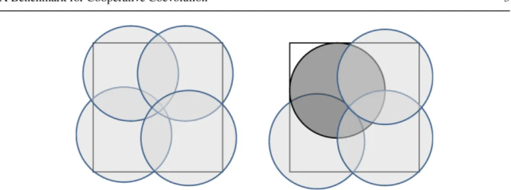
Fig. 1 Placement of a set of lamps. The aim is to enlighten all the square area. It is interesting to notice how a solution where some of the light of each lamp is wasted outside the area (left) overall performs better than a solution where the grayed lamp maximises its own performance (right).
Group Evolution, and Allopatric Group Evolution, is detailed in sections 3, 4 and 5 respectively. The experimental setup is described in section 6: four strategies are tested, a classical genetic programing approach, (CE for Classical Evolution), the Parisian Evolution (PE), the Group Evolution (GE) and the Allopatric Group Evo-lution (AGE). All methods are implemented using the µGP toolkit [24]. Results are presented and analysed in section 7, and conclusions and future work are given in section 8.
2 The Lamps problem
The optimisation problem chosen to test cooperative coevolution algorithms requires to find the best placement for a set of lamps, so that a target area is fully brightened with light. The minimal number of lamps needed is unknown, and heavily depends on the topology of the area. Lamps are all alike, modeled as circles, and each one may be evaluated separately with respect to the final goal. In the example, the optimal solu-tion requires 4 lamps (Figure 1, left): interestingly, when examined independently, all lamps in the solution waste a certain amount of light outside the target area. However, if one of the lamps is positioned to avoid this undesired effect, it becomes impossible to lighten the remaining area with the three lamps left (Figure 1, right). Since lamps are simply modeled as circles, the problem may also be seen as using the circles to completely cover the underlying area, as efficiently as possible.
This apparently simple benchmark exemplifies a common situation in real-world applications: many problems have an optimal solution composed of a set of homoge-neous elements, whose individual contribution to the main solution can be evaluated separately. Note that, in this context, homogeneous is used to label elements shar-ing the same base structure. Not only, but often the optimal solution is composed of not-optimal sub-solutions.
A similar toy problem has been sketched in [25]. Here the structure of the bench-mark is improved and parametrised, and a modified fitness function increases the complexity and the number of local optima on the fitness landscape.
2.1 Size of the problem
It is intuitive that the task of enlightening a room with a set of lamps can be more or less difficult, depending on the size of the room and the cone of light of each lamp. If small sources of light are used to brighten a large room, surely a greater number of lamps will be required, and the number of possible combinations will increase dramatically.
With these premises, the complexity of the problem can thus be expressed by the ratio between the surface to be enlightened and the maximum area enlightened by a single lamp:
problem size=area room
area lamp
as this ratio increases, finding an optimal solution for the problem will become harder. It is interesting to notice how variations in the shape of the room could also in-fluence the complexity of the task: rooms with an irregular architecture may require more intricate lamp placements. However, finding a dependency between the shape of the room and the difficulty of the problem is not trivial, and results might be less intuitive to analyze. Also, the cooperative coevolution algorithms do not search for or benefit from eventual symmetries in the problem. For all these reasons, the following experiments will feature square rooms only.
2.2 Fitness value
Comparing different methodologies on the same problem requires a common fitness function, to be able to numerically evaluate the efficiency of each approach.
Intuitively, the fitness of a candidate solution should be directly proportional to the area fully brightened by the lamps and inversely proportional to the number of lamps used, favoring solutions that cover more surface with light using the minimal number of lamps. The first term in the fitness value will thus be proportional to the ratio of the area enlightened by the lamps,
area enlightened total area
A further contribution is added, to help experts in evaluating the goodness of the grouping performed by the algorithms: the area brightened by more than one lamp is to be minimised, in order to have as little overlapping as possible. The second term will be then proportional to:
−area overlap
total area
It is interesting to note that minimising the overlap also implies an optimisation of the number of lamps used, since using a greater number would lead to more overlapping areas.
The final fitness function will then be:
f itness=area enlightened
total area −W ·
area overlap
total area =
=area enlightened−W · area overlap
total area
where W is a weight associated to the relative importance of the overlapping, set by the user.
Using this function with W = 1, fitness values will range between (0, 1), but it is intuitive that it is impossible to reach the maximum value: by problem construction, overlapping and enlightenment are inversely correlated, and even good solutions will feature overlapping areas and/or parts not brightened. This problem is actually multi-objective, the fitness function we propose corresponds to a compromise between the two objectives.
3 Parisian Evolution
Initially designed to address the inverse problem for Iterated Function System (IFS), a problem related to fractal image compression[10], this scheme has been successfully applied in various real world applications: in stereovision [6], in photogrammetry [12, 18], in medical imaging [27], for Bayesian Network Structure learning [4], in data retrieval[17].
Parisian Evolution (PE) is based on a two-level representation of the optimisa-tion problem, meaning that an individual in a Parisian populaoptimisa-tion represents only a part of the solution. An aggregation of multiple individuals must be built to com-plete a meaningful solution to the problem. This way, the co-evolution of the whole population (or of a major part of it) is favoured over the emergence of a single best individual, as in classical evolutionary schemes.
This scheme distributes the workload of solution evaluations at two levels. Light computations (e.g. existence conditions, partial or approximate fitness) can be done at the individual’s level (local fitness), while the complete calculation (i.e. global fitness) is performed at the population level. The global fitness is then distributed as a bonus to individuals who participate the global solution. A Parisian scheme has all the features of a classical EA (see figure 2) with the following additional components: – A grouping stage at each generation, that selects individuals that are allowed to
participate to the global solution.
– A redistribution step that rewards the individuals who participate to the global solution : their bonus is proportional to the global fitness.
– A sharing scheme, that avoids degenerate solutions where all individuals are iden-tical.
Efficient implementations of the Parisian scheme are often based on partial re-dundancies between local and global fitness, as well as clever exploitation of com-putational shortcuts. The motivation is to make a more efficient use of the evolution
Selection Crossover Mutation PARENTS Elitism OFFSPRING
Extraction of the solution Initialisation
Feedback to individuals Aggregate solutions
(global evaluation)
(local evaluation)
Fig. 2 A Parisian EA: a monopopulation cooperative-coevolution. Partial evaluation (local fitness) is ap-plied to each individual, while global evaluation is performed once a generation.
of the population, and reduce the computational cost. Successful applications of such a scheme usually rely on a lower cost evaluation of the partial solutions (i.e. the in-dividuals of the population), while computing the full evaluation only once at each generation or at specified intervals.
3.1 Implementation of the lamps problem
For the lamps problem, the PE has been implemented as follows. An individual rep-resents a lamp: its genome is its position, a pair of real values (x, y), plus a third element, e, that can assume values 0 or 1 (on/off switch). Lamps with e = 1 are “on” (expressed) and contribute to the global solution, while lamps with e = 0 do not.
Global fitness is computed as described in subsection 2.2. In generation 0 the global solution is computed simply considering the individuals with e = 1 among the µ initial ones. Then, at each step, λ individuals are generated. For each new individual with e = 1, its potential contribution to the global solution is computed. Before evaluation, a random choice (p = 0.5) is performed: new individuals are either considered in addition to or in replacement of the existing ones.
If individuals are considered for addition, the contribution to the global solution of each one is computed. Otherwise, the less performing among the old individu-als is removed, and only then the contribution to the global solution of each new individual is evaluated. If the addition or replacement of the new individuals leads to an improvement over the previous global fitness, the new individual selected is rewarded with a high local fitness value (local f itness = 2), together with all the old individuals still contributing to the global solution. New expressed individuals (e = 1) that are not selected for the global solution are assigned a low fitness value (local f itness = 0). Non-expressed individuals (e = 0) have an intermediate fitness value (local f itness = 1).
Sharing follows the simple formula
f itness sharing(Ik) =
local f itness(Ik)
with
sharing(I1, I2) =
(
1 − d(I1,I2)
2·lamp radius d(I1, I2) < 2 · lamp radius
0 d(I1, I2) ≥ 2 · lamp radius
Lamps that have a relatively low number of neighbours will be preferred for selection over lamps with a bigger number of neighbours. In this implementation, sharing is computed only for expressed lamps (e = 1) and used only when selecting the less performing individual to be removed from the population.
4 Group Evolution
Group Evolution (GE) is a novel generational cooperative coevolution concept pre-sented in [25]. The approach uses a population of partial solutions, and exploits non-fixed sets of individuals called groups. GE acts on individuals and groups, managing both in parallel. During the evolution, individuals are optimised as in a common EA, but concurrently groups are also evolved. The main peculiarity of GE is the absence of a priori information about the grouping of individuals.
At the beginning of the evolutionary process, an initial population of individuals is randomly created on the basis of a high-level description of a solution for the given problem. Groups at this stage are randomly determined, so that each individual can be included in any number of different groups, but all individuals are part of at least one group.
The number of groups µgroups, the minimum and maximum size of the groups are
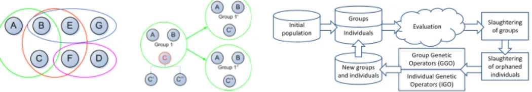
set by the user before the evolution starts. The number of individuals in the population is a direct consequence of the specified values for groups. Figure 3 (left) shows a sample population where minimum group size is 2, and maximum group size is 4.
Group Genetic Operators (GGO) Individual Genetic Operators (IGO) New groups and individuals Slaughtering of orphaned individuals Slaughtering of groups Evaluation Individuals Groups Initial population
Fig. 3 (Left) Individuals and Groups in a sample population of 8 individuals. While individual A is part of only one group, Individual B is part of 3 different groups. The effect of a Individual Genetic Operator, applied to individual C. Since individual C is part of Group 1, two groups are created and added to the population. (Right) Schema of Group Evolution algorithm. Groups are sets of individuals. At each step, new groups and individuals are produced. The slaughtering is performed at the level of groups, and in a second step individuals that are not included in any group are also removed.
4.1 Generation of new individuals and groups
GE exploits a generational approach: at each evolutionary step, a number of genetic operators is applied to the population. Genetic operators can act on both
individu-als and groups, and produce a corresponding offspring, in form of individuindividu-als and groups.
The offspring creation phase comprehends two different actions at each genera-tion step (see Figure 3):
1. Application of group genetic operators; 2. Application of individual genetic operators.
Each time a genetic operator is applied to the population, parents are chosen and offspring is generated. The children are added to the population, while the original parents are unmodified. Offspring is then evaluated, while it is not compulsory to reconsider the fitness value of the parents again. It is important to notice that the number of children produced at each evolutionary step is not fixed: each genetic op-erator can have any number of parents as input and produce in output any number of new individuals and groups. The number and type of genetic operators applied at each step can be set by the user.
4.1.1 Group genetic operators
Group Genetic Operators (GGOs) work on the set of groups. Each operator needs a certain number of groups as parents and produces a certain number of groups as offspring that will be added to the population. GGOs implemented in our approach are:
1. crossover: generates offspring by selecting two individuals, one from parent group A and one from parent group B. Those individuals are switched, creating two new groups;
2. add-mutation: generates offspring by selecting one or more individuals from the population and a group. Chosen individuals are added (if possible) to the parent group, creating a single new group;
3. removal-mutation: generates offspring by selecting a group and one or more individuals inside it. Individuals are removed from the parent group.
4. replacement-mutation: generates offspring by selecting a group and one or more individuals inside it. Individuals are removed from the parent group, and replaced by other individuals selected from the population.
Parent groups are chosen via tournament selection.
4.1.2 Individual genetic operators
Individual Genetic Operators (IGOs) operate on the population of individuals, very much like they are exploited in usual GA. The novelty of GE is that for each individ-ual produced as offspring, new groups are added to the group population. For each group the parent individual was part of, a copy is created, with the offspring taking the place of the parent.
This approach, however, could lead to an exponential increase in the number of groups, as the best individuals are selected by both GGOs and IGOs. To keep the
number of groups under a strict control, we choose to create a copy only of the highest-fitness groups the individual was part of.
IGOs select individuals by a tournament selection in two parts: first, a group is picked out through a tournament selection with moderate selective pressure; then an individual in the group is chosen with low selective pressure. The actual group and the highest-fitness groups the individual is part of are cloned once for each child individual created: in each clone group the parent individual is replaced with a child. An example is given in Figure 3 (right): an IGO, selects individual C as a parent. The chosen individual is part of only one group, Group 1. The IGO produces two children individuals: since the parent was part of a group, a new group is created for each new individual generated. The new groups (Group 1’ and Group 1”) are identical to Group 1, except that individual C is replaced with one of its children, C’ in Group 1’ and C” in Group 1” respectively.
The aim of this process is to select individuals from well-performing groups to create new groups with a slightly changed individual, in order to explore the a near area in the solution space.
4.2 Evaluation
During the evaluation phase, a fitness value is associated to each group: the fitness value is a number that measures the goodness of the candidate solutions with respect to the given problem. When a group is evaluated, a fitness value is also assigned to all the individuals composing it. Those values reflect the goodness of the solution represented by the single individual and have the purpose to help discriminate during tournament selection for both IGOs and GGOs.
An important strength of the approach resides in the evaluation step: if there is already a fitness value for an individual that is part of a new group, it is possible to take it into account instead of re-evaluating all the individuals in the group. This feature can be exceptionally practical when facing a problem where the evaluation of a single individual can last several minutes and the fitness of a group can be computed without examining simultaneously the performance of the individuals composing it. In that case, the time-wise cost of both IGOs and GGOs becomes very small.
4.3 Slaughtering
After each generation step, the group population is resized. The groups are ordered fitness-wise and the worst one is deleted until the desired population size is reached. Every individual keeps track of all the groups it belongs to in a set of references. Each time a group ceases to exist, all its individuals remove it from their set of references. At the end of the group slaughtering step, each individual that has an empty set of references, and is therefore not included in any group, is deleted as well.
4.4 Implementation of the lamps problem
For the lamps problem, GE has been implemented as follows. One individual rep-resents a lamp: its genome is its position, a pair of real values (x, y). The fitness of a single individual, which must be independent from all groups it is part of, is sim-ply the area of the room it enlightens. The group fitness is computed as described in subsection 2.2.
5 Allopatric Group Evolution
The third proposed cooperative coevolution algorithm stems from the Group Evolu-tion presented in the previous SecEvolu-tion. While the flow of the algorithm is the same, however, two major improvements distinguish the Allopatric Group Evolution from the previously described methodology: allopatric group slaughtering and heuristic group genetic operators.
5.1 Allopatric group slaughtering
Allopatric speciation (from the ancient Greek allos, other, and patra, fatherland) is a speciation that occurs when biological populations of the same species become iso-lated, usually due to geographical changes, such as major changes in the landscape.
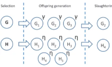
Taking inspiration from this natural phenomenon, the allopatric group slaughter-ing temporarily isolates from the main population all the offsprslaughter-ing of a group. Subse-quently, the offspring compete between themselves, and only the best resulting group is added back into the main population. A summary of the technique is presented in Figure 4.
Fig. 4 Allopatric slaughtering of groups. Group G and group H are chosen for reproduction in the same iteration. The operator applied to group G creates three children groups, with the allopatric tag γ, while the operator applied to group H creates five, with tag η. Among all the offspring that share the same allopatric tag, only the best group is added to the population: in the example, the fitness value of offspring H3might
be higher than the value of G2; nevertheless, G2is the best group among the offspring of G.
This mechanism is aimed at improving diversity, trying to avoid the invasion of the main group population by the offspring of a particularly promising group, an event that could drive the evolution deep into a local optima.
5.2 Heuristic group operators
The second important difference between AGE and GE, is the presence of heuris-tic group operators. The aim of the operators is to exploit expert knowledge of the problem that cannot be incorporated inside the group or individual fitness function. In the current implementation, two heuristic operators substitute removal-mutation and add-mutation presented in Subsection 4.1.1. When an individual is chosen to be removed from or added to a group, instead of a simple random selection, an external heuristic selector chooses the best candidate, according to a metric specified by the user.
Heuristic operators might prove beneficial to the evolution, especially when a run of the selector is not as computationally expensive as the evaluation of a group.
5.3 Implementation of the lamp problem
The setup is the same as in GE, with the only necessary addition of a heuristic to add or remove individuals from a group. For the lamp problem, we exploited the distance between individuals as an intuitive measurement of possible overlap. In particular, candidate individuals to be added to a group are evaluated on their distance from the nearest component of a group; while candidate individuals to be removed from a group are evaluate on the sum of the distances from the other components of the group.
6 Experimental setup
Before starting the experiments on the cooperative coevolution algorithms, a series of 10 runs for each problem size of a classical evolutionary algorithm is performed, to better understand the characteristics of the problem and to set parameters leading to a fair comparison. The genome of a single individual is a set of lamps, modeled
as an array of N pairs of real values ((x1, y1), (x2, y2), ..., (xN, yN)), where each (xi, yi)
describes the position of individual i in the room. The algorithm uses a classical (µ + λ ) evolutionary paradigm, with µ = 20 and λ = 10, probability of crossover 0.2 and probability of mutation 0.8. Each run lasts 100 generations.
By examining these first experimental results, it is possible to reach the following conclusions: good solutions for the problem use a number of lamps in the range (problem size, 3 · problem size); and, as expected, as the ratio grows, the fitness value of the best individual at the end of the evolution tends to be lower.
In order to perform a comparison with PE, GE and AGE as fair as possible, the stop condition for each algorithm will be set as the average number of single lamp evaluations performed by the classical evolutionary algorithm for each problem size. In this way, even if the algorithms involved have significantly different structures, the computational effort is commensurable. The number of evaluation ranges is 3, 500 for problem size = 3; 5, 000 for problem size = 5; 11, 000 for problem size = 10; 22, 000 for problem size = 20; and 120, 000 for problem size = 100.
6.1 PE setup
Due to the observation of the CE runs, µ = 3 · problem size, while λ = µ/2. The probability of mutation is 0.8 and the probability of crossover is 0.2.
6.2 GE and AGE setup
The number of groups in the population is fixed, µgroups= 20, as is the number of
genetic operators selected at each step λ = 10. The number of individuals in each group is set to vary in the range (problem size, 3 · problem size). The probability of mutation is 0.8, while the probability of crossover is 0.2, for both individuals and groups.
6.3 Implementation in µGP
The two CCEAs used in the experience have been implemented using µGP [24], an evolutionary toolkit developed by CAD group of Politecnico di Torino. Exploiting µ GP’s flexible structure, it is possible to replicate the behavior of very different EAs. In particular, to implement PE, it is sufficient to operate on the fitness evaluator, setting the environment to evaluate the whole population and the offspring at each step. Obtaining GE behavior is slightly more complex, and requires the addition of new classes to manage groups. CE is simply µGP standard operation mode.
The individual-level operators chosen for the experience are
singleParameter-AlterationMutationand onePointCrossover. The mutation operator acts
on one or both coordinates of a single individual, modifying them according to a gaus-sian distribution and producing a single child. The crossover operator, on the other
hand, starting from two individuals A = (xa, ya) and B = (xb, yb), creates two children
individuals AB = (xa, yb) and BA = (xb, ya). For further information, see [24].
7 Results and Analysis
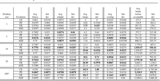
In a series of experiments, 100 runs of each evolutionary approach are executed, for a set of meaningful values of problem size. To exploit a further measurement of com-parison, the first occurrence of an acceptable solution also appears in the results: here an acceptable solution is defined as a global solution with at least 80% of the final fitness value obtained by the CE. Table 1 summarises the results for significant values of problem size. For each evolutionary algorithm are reported the results reached at the end of the evolution: average fitness value, average enlightenment percentage of the room, average number of lamps, and average number of lamps evaluated before finding an acceptable solution (along with the standard deviation for each value).
Results distributions are compared with a standard Student t-test, with no as-sumptions on the homogeneity of the standard deviations. Entries in bold in Table 1 are significantly better (p < 0.05) than others in the same column, for the same problem size.
Avg. lamps
Problem Avg. Std Avg. Std Avg. Std Avg. Std before Std
size Evolution fitness dev enlight. dev lamps dev overlap dev acceptable dev
3 CE 0.861 0.0149 0.8933 0.0212 4 0 0.0323 0.0168 313.2 126 PE 0.8355 0.064 0.8945 0.0439 4.02 0.3344 0.059 0.0502 316.9 262.2 GE 0.8764 0.0498 0.8963 0.0533 3.75 0.435 0.0198 0.0103 267.32 138.1 AGE 0.8507 0.0263 0.8998 0.0271 4.2 0.324 0.049 0.0266 349.65 179.21 5 CE 0.7802 0.023 0.8574 0.04 6.2 0.64 0.0772 0.0278 572.7 215.38 PE 0.7825 0.03 0.8803 0.0335 6.96 0.6936 0.0978 0.0395 511.35 373.85 GE 0.8136 0.0241 0.8537 0.0349 6.03 0.7372 0.0401 0.0166 741.36 221.86 AGE 0.79 0.0234 0.8875 0.0303 7.24 0.6624 0.0975 0.03189 608.32 255.75 10 CE 0.7487 0.0149 0.834 0.0235 11.3 0.62 0.0853 0.0216 1,779.8 407.4 PE 0.7791 0.0221 0.8847 0.0207 12.84 0.8184 0.1055 0.0274 1,018.47 546.16 GE 0.7532 0.0178 0.8132 0.0255 10.66 0.6336 0.0599 0.0215 1,836.87 412.08 AGE 0.75 0.017 0.866 0.0229 13.09 0.8352 0.1159 0.0251 1,715.85 637.91 20 CE 0.6804 0.0117 0.7749 0.0148 20.6 0.72 0.0946 0.0123 3,934.7 702.24 PE 0.7624 0.0147 0.8762 0.0168 23.57 1.053 0.1138 0.0177 2,759.28 965.45 GE 0.697 0.0127 0.7837 0.0147 20.49 0.5978 0.0867 0.0142 4,602.1 1,156.5 AGE 0.7086 0.0182 0.8523 0.0269 25.14 1.514 0.1437 0.0293 3,151.31 1,067.89 100* CE 0.558 0.0049 0.7334 0.0062 102.9 1.88 0.1755 0.0093 29,567.3 4,782.96 PE 0.6867 0.0073 0.8708 0.0078 117.2 3.2 0.1841 0.0134 5,318.9 332.72 GE 0.5647 0.0057 0.7309 0.0073 101.5 1.7 0.1662 0.0072 30,048 8,876.8 AGE 0.6095 0.021 0.792 0.0314 111.4 9.2 0.1824 0.04 12,094.4 3,686.28
Table 1 Average results for 100 runs, for each evolutionary approach. For problem size = 100, the distri-bution of AGE presents such a vast standard deviation that it is not distinguishable from the other three approaches (p > 0.05). Taking into account the remaining three distributions, GE is the best (p < 0.05). *Due to the times involved, data for problem size 100 is computed on 10 runs.
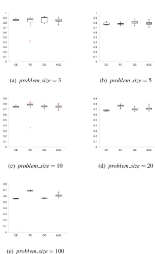
For each problem size, a box plot is provided in figure 5. It is noticeable how the performance of each evolutionary algorithm is very close for small values of problem size, while PE, GE and AGE gain the upper hand when the complexity increases.
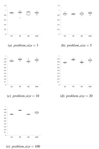
In particular, PE obtains the best performance from problem size = 10 onwards. The extra information inserted allows the approach to obtain high enlightenment per-centages even when the complexity of the task increases, as shown in Figure 6.
On the other hand, GE obtains enlightenment percentages close to CE, but on the average it uses a lower number of lamps, that leads to a lower overlap, as it is noticeable in Figure 8 and 7.
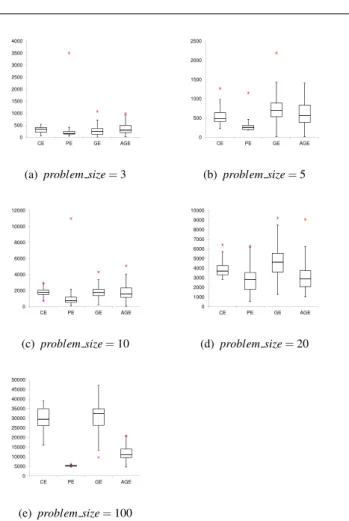
When dealing with the number of lamp evaluations needed before reaching what is defined an acceptable solution, PE is again in the lead, see Figure 9.
In Figure 10, a profile of the best run for problem size = 100 for each algorithm is reported. PE enjoys a rapid growth in the first stages of the evolution, thanks to the extra information it can make use of, while GE proves more efficient than CE in the last part of the evolution, where exploitation becomes more prevalent. AGE shows several steep improvements, in correspondence of a particularly successful activation of the heuristic group operators.
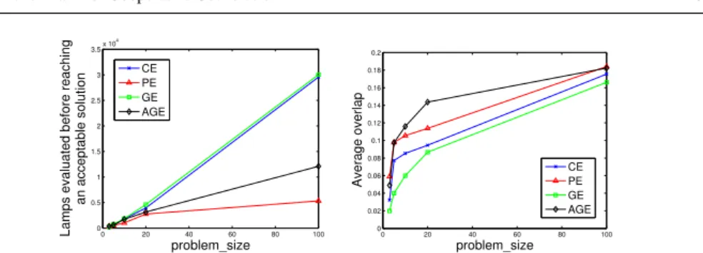
As it is noticeable in Figure 11 (left), while the number of lamps evaluated before reaching an acceptable solution grows more than linearly for CE and GE, AGE shows a less steep growth and PE outperforms all the other algorithms. On the other hand, GE presents the lowest overlap for all values of problem size, see Figure 11 (right).
8 Conclusion and future work
The lamps benchmark has the major advantage to provide a set of toy problems that are simple, and for which the complexity can be characterised with a single real value
0.4 0.5 0.6 0.7 0.8 0.9 1 0 0.1 0.2 0.3 0.4 CE PE GE AGE
(a) problem size = 3
0.4 0.5 0.6 0.7 0.8 0.9 1 0 0.1 0.2 0.3 0.4 CE PE GE AGE (b) problem size = 5 0.4 0.5 0.6 0.7 0.8 0.9 0 0.1 0.2 0.3 CE PE GE AGE (c) problem size = 10 0.4 0.5 0.6 0.7 0.8 0.9 0 0.1 0.2 0.3 CE PE GE AGE (d) problem size = 20 0.3 0.4 0.5 0.6 0.7 0.8 0 0.1 0.2 0.3 CE PE GE AGE
(e) problem size = 100
Fig. 5 Box plots of fitness values for each problem size.
(the surface ratio between room and lamp sizes). This formulation is very convenient to get some insight on the behaviour of algorithms with respect to the size of the problem.
The intuition that guided the development of Parisian Evolution, Group Evolu-tion and Allopatric Group EvoluEvolu-tion has been confronted to experimental analysis, to yield the following conclusions: Parisian Evolution is the most efficient approach in terms of computational expense, and scalability; Group Evolution yields better and more precise results, in a computational time that is similar to Classical Evolution; Allopatric Group Evolution shows a behavior that is intermediate between the two, obtaining some advantage over GE for higher complexities of the problem, but fail-ing to meet Parisian Evolution’s performance. In general, AGE solutions also present a considerable standard deviation, probably because the combination of heuristics and evolutionary operators drives the evolution in very different niches of the search space, depending on the single run.
0.6 0.8 1 1.2 0 0.2 0.4 CE PE GE AGE
(a) problem size = 3
0.6 0.8 1 1.2 0 0.2 0.4 CE PE GE AGE (b) problem size = 5 0.4 0.5 0.6 0.7 0.8 0.9 1 0 0.1 0.2 0.3 0.4 CE PE GE AGE (c) problem size = 10 0.4 0.5 0.6 0.7 0.8 0.9 1 0 0.1 0.2 0.3 0.4 CE PE GE AGE (d) problem size = 20 0.4 0.5 0.6 0.7 0.8 0.9 1 0 0.1 0.2 0.3 0.4 CE PE GE AGE
(e) problem size = 100
Fig. 6 Box plots of enlightenment percentage for each problem size.
These differences can be explained by the nature of a priori information that has been injected into the algorithms. Parisian Evolution relies on a deterministic algorithm for selecting the group of lamps that are used as the current global solution at each generation, while Group Evolution does not make any assumption on it and let evolution decide which lamps can be grouped to build various solutions. Allopatric Group Evolution is a first attempt to make use of expert knowledge while avoiding a strong algorithmic choice, by adding information at the level of its heuristic genetic operators: the chosen metrics, however, show a variable performance, dependent on the size of the problem.
In some sense Parisian Evolution is making a strong algorithmic choice for the grouping stage, that acts as a constraint on the evolution of the population of lamps. It has the major advantage to reduce the complexity of the problem by providing solutions from the evolution of simpler structures (lamps instead of groups of lamps for both Allopatric and standard Group Evolution, or for Classical Evolution). It may be considered as a “quick and dirty” approach.
3 4 5 6 7 0 1 2 CE PE GE AGE
(a) problem size = 3
4 5 6 7 8 9 10 0 1 2 3 4 CE PE GE AGE (b) problem size = 5 10 15 20 25 0 5 10 CE PE GE AGE (c) problem size = 10 15 20 25 30 35 0 5 10 CE PE GE AGE (d) problem size = 20 60 80 100 120 140 0 20 40 CE PE GE AGE
(e) problem size = 100
Fig. 7 Box plots of number of lamps used for each problem size.
Future work on this topic will investigate other possible compromises between heuristics and evolution: a promising option is an hybridisations between Parisian and Group Evolution, i.e. running a population of elements in the Parisian mode to rapidly get a good rough solution, and using the Group scheme to refine it. A more realistic modeling of the lamp’s light could also be used, taking into account the gradual fading from the source; this approach would shift the problem from enlightening the room to ensure that each point of it receives at least a certain amount of light.
9 Acknowledgments
Aknowledgements for the funding received from the European Community’s Sev-enth Framework Programme (FP7/2009-2013) under grant agreement DREAM n. 222654-2.
0.3 0.4 0.5 0.6 0 0.1 0.2 CE PE GE AGE
(a) problem size = 3
0.1 0.15 0.2 0.25 0 0.05 0.1 CE PE GE AGE (b) problem size = 5 0.3 0.4 0.5 0.6 0 0.1 0.2 CE PE GE AGE (c) problem size = 10 0.1 0.15 0.2 0.25 0 0.05 0.1 CE PE GE AGE (d) problem size = 20 0.15 0.2 0.25 0.3 0 0.05 0.1 CE PE GE AGE
(e) problem size = 100
Fig. 8 Box plots of overlap percentage for each problem size.
References
1. Ahluwalia M, Bull L (1998) Co-evolving functions in genetic programming: Dy-namic adf creation using glib. In: Evolutionary Programming, pp 809–818 2. Amaya JE, Cotta C, Fernndez AJ (2010) A memetic cooperative optimization
schema and its application to the tool switching problem. In: PPSN 2010, 11th International Conference on Parallel Problem Solving From Nature, September 11-15, Krakow, Poland, springer Verlag, Series: Lecture Notes in Computer Sci-ence, Vol. 6238 and 6239
3. Axelrod R (1984) The Evolution of Cooperation. Basic Books
4. Barri`ere O, Lutton E, Wuillemin PH (2009) Bayesian network structure learn-ing uslearn-ing cooperative coevolution. In: Genetic and Evolutionary Computation Conference (GECCO 2009)
5. Bongard J, Lipson H (2005) Active coevolutionary learning of deterministic fi-nite automata. Journal of Machine Learning Research 6:1651–1678
1500 2000 2500 3000 3500 4000 0 500 1000 1500 CE PE GE AGE
(a) problem size = 3
1000 1500 2000 2500 0 500 1000 CE PE GE AGE (b) problem size = 5 6000 8000 10000 12000 0 2000 4000 CE PE GE AGE (c) problem size = 10 4000 5000 6000 7000 8000 9000 10000 0 1000 2000 3000 4000 CE PE GE AGE (d) problem size = 20 20000 25000 30000 35000 40000 45000 50000 0 5000 10000 15000 20000 CE PE GE AGE
(e) problem size = 100
Fig. 9 Box plots of number of lamps evaluated before reaching an acceptable solution, for each problem size. 0 2 4 6 8 10 12 14 x 104 0.25 0.3 0.35 0.4 0.45 0.5 0.55 0.6 0.65 0.7 0.75
Number of lamps evaluated
Fitness value
Profile of the best run for problem_size = 100
CE PE GE AGE
Fig. 10 Profile of the best run for each evolutionary algorithm at problem size = 100.
6. Boumaza AM, Louchet J (2001) Dynamic flies: Using real-time parisian evolu-tion in robotics. In: Boers EJ, Cagnoni S, Gottlieb J, Hart E, Lanzi PL, Raidl G, Smith RE, Tijink H (eds) Applications of Evolutionary Computing. EvoWork-shops2001: EvoCOP, EvoFlight, EvoIASP, EvoLearn, and EvoSTIM. Proceed-ings, Springer-Verlag, Como, Italy, LNCS, vol 2037, pp 288–297
0 20 40 60 80 100 0 0.5 1 1.5 2 2.5 3 3.5x 10 4 problem_size
Lamps evaluated before reaching
an acceptable solution CE PE GE AGE 0 20 40 60 80 100 0 0.02 0.04 0.06 0.08 0.1 0.12 0.14 0.16 0.18 0.2 problem_size Average overlap CE PE GE AGE
Fig. 11 (Left) Average number of lamps evaluated before reaching an acceptable solution, for different values of problem size. (Right) Average overlap of the final solution, for different values of problem size.
7. Bucci A, Pollacj JB (2005) On identifying global optima in cooperative coevolu-tion. In: GECCO ’05: Proceedings of the 2005 conference on Genetic and evo-lutionary, Washington DC, USA
8. Chen W, Weise T, Yang Z, Tang K (2010) Large-scale global optimization using cooperative coevolution with variable interaction learning. In: PPSN 2010, 11th International Conference on Parallel Problem Solving From Nature, September 11-15, Krakow, Poland, springer Verlag, Series: Lecture Notes in Computer Sci-ence, Vol. 6238 and 6239
9. Collet P, Lutton E, Raynal F, Schoenauer M (1999) Individual gp: an alternative viewpoint for the resolution of complex problems. In: GECCO99, Genetic and Evolutionary Computation Conference, July 13 - 17, 1999, Orlando, Florida, USA.
10. Collet P, Lutton E, Raynal F, Schoenauer M (2000) Polar ifs + parisian genetic programming = efficient ifs inverse problem solving. Genetic Programming and Evolvable Machines Journal 1(4):339–361, october
11. De Jong ED, Stanley KO, Wiegand RP (2007) Introductory tutorial on coevolu-tion. In: GECCO ’07: Proceedings of the 2007 GECCO conference companion on Genetic and evolutionary computation, London, United Kingdom
12. Dunn E, Olague G, Lutton E (2005) Automated photogrammetric network design using the parisian approach. In: EvoIASP 2005, Lausanne, nominated for the best paper Award
13. Holland JH, Reitman JS (1978) Cognitive systems based on adaptive algorithms. In: Waterman DA, Hayes-Roth F (eds) Pattern directed inference systems, Aca-demic Press, pp 313–329
14. Husbands P, Mill F (1991) Simulated co-evolution as the mechanism for emer-gent planning and scheduling. In: ICGA, Proceedings of the 4th International Conference on Genetic Algorithms, San Diego, CA, USA, pp 264–270
15. Husbands P, Mill F (1991) Simulated co-evolution as the mechanism for emer-gent planning and scheduling. In: Belew R, Booker L (eds) Proceedings of the 4th International Conference on Genetic Algorithms, Morgan Kaufmann 16. Kauffman SA, Johnsen S (1991) Coevolution to the edge of chaos: Coupled
fit-ness landscapes, poised states, and coevolutionary avalanches. Journal of Theo-retical Biology 149(4):467 – 505
17. Landrin-Schweitzer Y, Collet P, Lutton E (2006) Introducing lateral thinking in search engines. GPEM, Genetic Programming an Evolvable Hardware Journal, W Banzhaf et al Eds 1(7):9–31
18. Lutton E, Olague G (2006) Parisian camera placement for vision metrology. Pat-tern Recognition Letters 27(11):1209–1219
19. Ochoa G, Lutton E, Burke EK (2007) Cooperative royal road functions. In: Evo-lution Artificielle, Tours, France, October 29-31
20. Panait L, Luke S, Harrison JF (2006) Archive-based cooperative coevolutionary algorithms. In: Proceedings of the 8th annual conference on Genetic and evolu-tionary computation, Seattle, Washington, USA
21. Popovici E, De Jong K (2006) The effects of interaction frequency on the op-timization performance of cooperative coevolution. In: Proceedings of the 8th annual conference on Genetic and evolutionary computation, Seattle, Washing-ton, USA
22. Potter MA, Couldrey C (2010) A cooperative coevolutionary approachto parti-tional clustering. In: PPSN 2010, 11th Internaparti-tional Conference on Parallel Prob-lem Solving From Nature, September 11-15, Krakow, Poland, springer Verlag, Series: Lecture Notes in Computer Science, Vol. 6238 and 6239
23. Potter MA, Jong KAD (1994) A cooperative coevolutionary approach to function optimization. In: PPSN, pp 249–257
24. Sanchez E, Schillaci M, Squillero G (2011) Evolutionary Optimization: the µGP toolkit, 1st edn. Springer
25. Sanchez E, Squillero G, Tonda A (2011) Group evolution: Emerging synergy through a coordinated effort. In: Proceedings of the 2011 IEEE Congress of Evo-lutionary Computation (CEC)
26. Tonda A, Lutton E, Squillero G (2012) Lamps: A test problem for cooperative coevolution. In: Pelta D, Krasnogor N, Dumitrescu D, Chira C, Lung R (eds) Nature Inspired Cooperative Strategies for Optimization (NICSO 2011), Studies in Computational Intelligence, vol 387, Springer Berlin / Heidelberg, pp 101–120 27. Vidal FP, Louchet J, Rocchisani JM, Lutton E (2010) New genetic operators in the fly algorithm: application to medical PET image reconstruction. In: Evolu-tionary Computation in Image Analysis and Signal Processing, EvoApplications 2010, Part I, LNCS 6024,C. Di Chio et al. (Eds.), Springer, 7th - 9th April, Istan-bul Technical University, IstanIstan-bul, Turkey
28. Wiegand RP, Potter MA (2006) Robustness in cooperative coevolution. In: Pro-ceedings of the 8th annual conference on Genetic and evolutionary computation, Seattle, Washington, USA
29. Wu S, Banzhaf W (2011) Rethinking multilevel selection in genetic program-ming. In: Proceedings of the 13th annual conference on Genetic and evolutionary computation, ACM, pp 1403–1410