1
Remerciements
Je souhaiterais ici chaleureusement remercier toutes les personnes qui ont contribué au bon déroulement de cette thèse de façon plus ou moins directe, par leur aide, leurs conseils ou leur soutien.
Merci tout d’abord à Jérôme Chave, mon directeur de thèse à Toulouse, pour m’avoir ouvert les portes de l’écologie, une discipline dont j’ignorais tout ou presque au début de ma thèse. Ayant été jusqu’alors principalement confronté à la recherche théorique, j’ai découvert un univers où les données, leur production, leur analyse et leur interprétation, sont le nerf de la guerre. Mon adaptation ne s’est pas faite en un jour, et je mesure aujourd’hui le chemin parcouru. Je te remercie Jérôme de tes efforts pour m’intégrer à la discipline en début de thèse, notamment en me permettant de partir deux fois faire du terrain aux Nouragues, une expérience inoubliable. Merci pour tes conseils toujours avisés et tes relectures attentives. Ton exigence, ton enthousiasme et ton énergie inépuisables, ton recul sur la discipline et ta large culture scientifique m’ont inspiré tout au long de ma thèse.
Merci à Hélène Morlon, ma directrice de thèse à Paris, de m’avoir accueilli pour ma dernière année de thèse. Outre que cette année supplémentaire m’a été précieuse pour terminer ma thèse dans de bonnes conditions, cette immersion dans la macro-évolution a été pour moi l’occasion de découvrir une autre façon d’aborder la recherche en écologie et évolution. Merci Hélène pour tes conseils, ton soutien et ta patience. Et merci de m’avoir fait profiter de cette atmosphère unique, où dynamisme, rigueur et efficacité riment si bien avec convivialité, bienveillance et décontraction. Nous n’avons pas eu l’occasion de travailler ensemble autant que je l’aurais souhaité au cours de cette thèse, et je me réjouis par conséquent de pouvoir continuer à le faire dans le futur.
I am very grateful to Christopher Quince and Corinne Vacher for taking the time to review this thesis. Thank you very much for your careful reading and your constructive criticism. I also thank Sébastien Brosse and Francesco Ficetola for agreeing to be part of the jury.
Merci à mes co-auteurs et collaborateurs, sur le travail desquels une grande partie de cette thèse est basée.
Merci en particulier à Lucie Zinger, dont le travail d’analyse et d’interprétation des données utilisées dans cette thèse a été crucial. Lucie, tu as été un précieux pont avec la biologie tout au long de cette thèse pour le physicien de formation que je suis, et je te suis infiniment reconnaissant pour tes nombreuses explications et conseils. Merci à Pierre Taberlet et Eric Coissac de m’avoir fait bénéficier de leur expertise state-of-the-art dans la production et l’analyse des données metabarcoding. Merci à Heidy Schimann pour son aide dans l’interprétation biologique des données, ainsi que pour son aide
2
préparation du terrain, sa contribution à la production des données, ainsi que pour sa remarquable efficacité pour surmonter les difficultés technique, logistique et administrative de tout ordre, le tout dans une bonne humeur inaltérable. Merci à Sophie Manzi et Eliane Louisanna pour leur aide sur le terrain et leur travail de wetlab. Merci à Vincent Schilling pour sa contribution aux analyses bioinformatiques, son aide sur le terrain, et pour son humour en tant que camarade de carbet aux Nouragues. Merci également à Saint Omer Cazal et Audrey Sagne pour leur aide sur le terrain à Paracou et Arbocel, et à Daniel Boutaud pour ses très utiles porte-piochons tout-terrain. Merci enfin à Elodie Courtois et Blaise Tymen de m’avoir fait découvrir la Guyane et les Nouragues en début de thèse, et pour ces moments partagés sur le terrain.
Je remercie en outre Antoine Fouquet et Jean-Pierre Vacher de m’avoir fait confiance pour l’analyse de leurs données. Merci également à Hélène Holota pour son efficacité, sa disponibilité et sa gentillesse, à Blaise Tymen pour son aide avec les données Lidar, et à Mélanie Roy, Antoine Fouquet, Gaël Grenouillet et Lounès Chikhi, entre autres, pour d’enrichissantes discussions et pour leurs conseils.
Je voudrais ensuite remercier un certain nombre de personnes qui, si elles n’ont pas directement contribué au contenu de cette thèse, ont éclairé mes journées de travail à Toulouse et Paris et ont fait le sel de ces quatre années de vie.
Merci à mes co-bureaux toulousains Jessica et Félix pour toutes ces longues discussions, et pour avoir supporté mon humour avec bienveillance en toute circonstance. Merci à mes quatre « camarades de promo » à EDB, Arthur, Paul, Isabelle et Jean-Pierre, avec qui cela a été un immense plaisir de partager ces trois années à Toulouse. Merci à Boris, Blaise, Mathieu, Olivia, Léa, Josselin, Aurèle, Luc, Nico, Camille, Céline, Marine, Lucie, Alice, Sébastien, Jade, Kévin, Jan, Fabian, Isabel … pour tous ces moments partagés, et à tous les membres d’EDB jeunes et moins jeunes pour l’ambiance remarquable du labo.
Merci à Simon et aux locataires successifs de l’inénarrable maison de la culture François Magendie, à Louise et ses plongées dans le monde du théâtre, à Etienne et Mathilde et leurs « écoles d’été » hippies, à Guillem, Claire, Hélène, Lucie, Lisa-Lou et aux autres, pour avoir brillamment peuplé ces années toulousaines. Merci à Jean-Pierre et Sébastien de m’avoir initié à l’herpéto. Merci à Alex pour son accueil à Montpellier et ces débats passionnés sur la science et l’écologie. Merci aux Américains : Marc et Léo et leur inspirant « Silicon Valley spirit », et Matthieu, fidèle birding buddy. Et merci à Simon et Florian pour leurs – trop rares – immersions dans l’informatique quantique et les réseaux d’énergie.
Un grand merci également à mes co-bureaux parisiens. Marc, Odile, Julien, Eric, Leandro, Olivier, votre accueil chaleureux dans et hors du labo a grandement facilité ma transition parisienne.
Merci enfin aux anciens, aux vieux de la vieille, Grenoblois d’ici et d’ailleurs : Thibault, Mathieu, Arantxa, David, Lucas, Aurore, Carl, Vio … Je vous compte parmi les amis, mais c’est déjà presque la famille.
Je remercie pour finir, last but not least, mes parents et mon frère, pour leur soutien sans faille et ô combien indispensable.
3 Introduction 5 I. What drives the assembly of ecological communities? 6 II. DNA-based biodiversity patterns 21 III. Statistical approaches 34 IV. Objectives and outline 53 Chapter 1 69 Causes of variation in soil beta diversity across domains of life in the tropical forests of French Guiana Chapter 2 113 Inferring neutral biodiversity parameters using environmental DNA data sets Chapter 3 163 Topic modelling reveals spatial structure in a DNA-based biodiversity survey Discussion 203 I. Synthesis 204 II. Perspectives 208 Appendix 221 Large-scale DNA barcoding of Amazonian anurans leads to a new definition of biogeographical subregions in the Guiana Shield and reveals a vast underestimation of diversity and local endemism
4
5
Introduction
Introduction 6
I. What drives the assembly of ecological
communities?
Science consists in finding patterns in a collection of isolated observations so as to gain understanding of the processes that generated them. Natural sciences began with attempts at classifying the diversity of the living organisms into categories (Aristotle, IVth cent. BC), and this classification has been developed and perfected over the centuries into the modern binomial nomenclature (Linnaeus, 1753). But classification efforts were not limited to the description of species. Associations of species, and in particular plant associations, were named using the same model, and were carefully described based on their taxonomic composition and the abiotic properties of their environment (Braun-Blanquet & Pavillard, 1922). Even though forest plant associations were observed shifting through time, this phenomenon was described as mirroring the life cycle of individual organisms, from ‘youth’ to ‘senescence’ (Clements, 1916). The underlying idea was that the organization of the living world obeyed static and deterministic rules, which were to be uncovered. This idea was encouraged by the discovery of the elegant laws that govern physics and chemistry.By contrast, early discoveries on evolution and biogeography (Darwin, 1859; Wallace, 1876) brought the idea that chance and history have played an overwhelming role in shaping the modern living world. Gleason (1926) and Tansley (1935) were the first to contend that the diversity of plant associations was not well described by discrete vegetation types, and that species associations were rather the transient outcome of random dispersal events, constrained by abiotic conditions and species interactions. Later, Hutchinson (1961), MacArthur (1972), Diamond (1975), Hubbell (1979), Ricklefs (1987), and Brown (1995), among others, have successively elaborated on this idea, laying the foundations of modern community ecology. The term ‘community’ refers to all the organisms coexisting in a given location and at a given time. It may also refer to a taxonomic subgroup of these organisms, such as a ‘plant community’.
7 The question of the relative role played by deterministic and stochastic processes in shaping ecological communities remains central to ecology. In this section, I first argue that addressing this question is key to our ability to preserve natural ecosystems and to predict their response to human perturbations. I then briefly review the mechanisms of community assembly that have been proposed. Motivations 1.
The increasing awareness of the threats posed to natural ecosystems by human activities has added a sense of urgency to the study of ecological processes. Indeed, the fate of the Earth’s biodiversity, and beyond it, of the ecosystems on which human societies rely for food, water, clean air, health, and raw materials, has become a major source of concern (Daily, 1997). As a consequence, theoretical advances in ecology can no longer be considered in isolation from their practical implications. In particular, many predictions relevant to policy-making strongly depend on assumptions regarding the mechanisms of community assembly. Thus, data-driven understanding of community assembly is critical to well-informed policy-making. Three examples are given below: the prediction of ecosystem stability and state shifts in response to human perturbations, the prediction of the impact of climate change, and the conservation of biodiversity.
Measuring ecosystem stability to perturbations is a subject of active research, as is the relationship between biodiversity and ecosystem stability (McCann, 2000; Tilman
et al., 2006; Loreau & de Mazancourt, 2013). In this context, natural ecosystems are
commonly represented as stable communities held together by species interactions, in part because this representation lends itself well to theoretical approaches (Arnoldi et
al., 2016). Drawing on this framework, it has been hypothesized that the response of
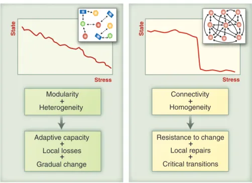
ecosystems to perturbations may bear a similarity with that of physical systems exhibiting critical phase transitions (cf. Fig. 1; Scheffer et al., 2012). Accordingly, ‘tipping points’, sudden and difficult-to-reverse shifts in a system’s state in response to
Introduction 8 perturbation, should be expected (Brook et al., 2013). Moreover, such state shifts could be possibly predicted in advance through the identification of early-warning signals (Carpenter et al., 2011; Scheffer et al., 2012). While this type of non-linear behaviour has been evidenced in lake ecosystems (Carpenter et al., 2011), it remains difficult to study empirically, and knowledge of community assembly processes is key to provide realistic assumptions for the theoretical prediction of possible tipping points.
Figure 1. The response of ecosystems to human-induced stress is commonly studied using a network representation of ecological communities, envisioned as stable entities held together by interactions. Depending on network connectivity and modularity, the response may be linear (left) or exhibit a tipping point (right). Data-driven knowledge of community assembly processes is much needed to inform such models. Adapted from Scheffer et al. (2012).
Climate change has become the foremost threat to many ecosystems, especially those that are less directly impacted by human activities. Species distribution modelling is an important tool to predict the effect of climate change on biodiversity (Miller, 2010). It consists in inferring the abiotic requirements of individual species from their observed geographic distribution, and predicting their future distribution based on predicted changes in abiotic conditions. The need to take into account processes other
Anticipating Critical Transitions
Marten Scheffer,1,2* Stephen R. Carpenter,3Timothy M. Lenton,4 Jordi Bascompte,5
William Brock,6Vasilis Dakos,1,5Johan van de Koppel,7,8Ingrid A. van de Leemput,1Simon A. Levin,9
Egbert H. van Nes,1Mercedes Pascual,10,11John Vandermeer10
Tipping points in complex systems may imply risks of unwanted collapse, but also opportunities for positive change. Our capacity to navigate such risks and opportunities can be boosted by combining emerging insights from two unconnected fields of research. One line of work is revealing fundamental architectural features that may cause ecological networks, financial markets, and other complex systems to have tipping points. Another field of research is uncovering generic empirical indicators of the proximity to such critical thresholds. Although sudden
shifts in complex systems will inevitably continue to surprise us, work at the crossroads of these emerging fields offers new approaches for anticipating critical transitions.
A
bout 12,000 years ago, the Earth sud-denly shifted from a long, harsh glacial episode into the benign and stable Hol-ocene climate that allowed human civilization to develop. On smaller and faster scales, ecosystems occasionally flip to contrasting states. Unlike grad-ual trends, such sharp shifts are largely unpre-dictable (1–3). Nonetheless, science is now carving into this realm of unpredictability in fundamental ways. Although the complexity of systems such as societies and ecological networks prohibits ac-curate mechanistic modeling, certain features turn out to be generic markers of the fragility that may typically precede a large class of abrupt changes. Two distinct approaches have led to these in-sights. On the one hand, analyses across networks and other systems with many components have revealed that particular aspects of their structure determine whether they are likely to have critical thresholds where they may change abruptly; on the other hand, recent findings suggest that cer-tain generic indicators may be used to detect if a system is close to such a “tipping point.” We high-light key findings but also challenges in theseemerging research areas and discuss how excit-ing opportunities arise from the combination of these so far disconnected fields of work.
The Architecture of Fragility
Sharp regime shifts that punctuate the usual fluc-tuations around trends in ecosystems or societies may often be simply the result of an unpredict-able external shock. However, another possibility is that such a shift represents a so-called critical transition (3, 4). The likelihood of such tran-sitions may gradually increase as a system ap-proaches a “tipping point” [i.e., a catastrophic bifurcation (5)], where a minor trigger can invoke a self-propagating shift to a contrasting state. One of the big questions in complex systems science is what causes some systems to have such tipping
points. The basic ingredient for a tipping point is a positive feedback that, once a critical point is passed, propels change toward an alternative state (6). Although this principle is well under-stood for simple isolated systems, it is more chal-lenging to fathom how heterogeneous structurally complex systems such as networks of species, habitats, or societal structures might respond to changing conditions and perturbations. A broad range of studies suggests that two major features are crucial for the overall response of such sys-tems (7): (i) the heterogeneity of the components and (ii) their connectivity (Fig. 1). How these properties affect the stability depends on the na-ture of the interactions in the network.
Domino effects. One broad class of networks includes those where units (or “nodes”) can flip between alternative stable states and where the probability of being in one state is promoted by having neighbors in that state. One may think, for instance, of networks of populations (extinct or not), or ecosystems (with alternative stable states), or banks (solvent or not). In such networks, het-erogeneity in the response of individual nodes and a low level of connectivity may cause the net-work as a whole to change gradually—rather than abruptly—in response to environmental change. This is because the relatively isolated and differ-ent nodes will each shift at another level of an en-vironmental driver (8). By contrast, homogeneity (nodes being more similar) and a highly connected network may provide resistance to change until a threshold for a systemic critical transition is reached where all nodes shift in synchrony (8, 9).
This situation implies a trade-off between lo-cal and systemic resilience. Strong connectivity
REVIEW
1Department of Environmental Sciences, Wageningen
Univer-sity, Post Office Box 47, NL-6700 AA Wageningen, Nether-lands.2South American Institute for Resilience and Sustainability
Studies (SARAS), Maldonado, Uruguay.3Center for Limnology,
University of Wisconsin, 680 North Park Street, Madison, WI 53706, USA. 4College of Life and Environmental Sciences,
University of Exeter, Hatherly Laboratories, Prince of Wales Road, Exeter EX4 4PS, UK.5Integrative Ecology Group, Estación
Biológica de Doñana, Consejo Superior de Investigaciones Científicas, E-41092 Sevilla, Spain.6Department of Economics,
University of Wisconsin, 1180 Observatory Drive, Madison, WI 53706, USA.7Spatial Ecology Department, Royal Netherlands
Institute for Sea Research (NIOZ), Post Office Box 140, 4400AC, Yerseke, Netherlands.8Community and Conservation Ecology
Group, Centre for Ecological and Evolutionary Studies (CEES), University of Groningen, Post Office Box 11103, 9700 CC Groningen, Netherlands.9Department of Ecology and
Evolu-tionary Biology, Princeton University, Princeton, NJ 08544–1003, USA.10University of Michigan and Howard Hughes Medical
Institute, 2045 Kraus Natural Science Building, 830 North Uni-versity, Ann Arbor, MI 48109–1048, USA.11Santa Fe Institute,
1399 Hyde Park Road, Santa Fe, NM 87501, USA.
*To whom correspondence should be addressed. E-mail: [email protected] Modularity Stress State State Stress Connectivity Heterogeneity
Adaptive capacity Resistance to change
Local losses Local repairs
Gradual change Critical transitions
+ +
Homogeneity
+ +
+ +
Fig. 1. The connectivity and homogeneity of the units affect the way in which distributed systems with local alternative states respond to changing conditions. Networks in which the components differ (are heterogeneous) and where incomplete connectivity causes modularity tend to have adaptive capacity in that they adjust gradually to change. By contrast, in highly connected networks, local losses tend to be “repaired” by subsidiary inputs from linked units until at a critical stress level the system collapses. The particular structure of connections also has important consequences for the robustness of networks, depending on the kind of interactions between the nodes of the network.
19 OCTOBER 2012 VOL 338 SCIENCE www.sciencemag.org
344
on July 20, 2017
http://science.sciencemag.org/
9 than abiotic requirements, such as species interactions, dispersal limitation, adaptation, and phenotypic plasticity, has long been acknowledged (Guisan & Thuiller, 2005), nevertheless most predictions are still obtained while ignoring these processes (Wisz et
al., 2013). Another approach to predicting the effect of climate change on ecosystems is
through the dynamical simulation of ecosystems, either by simulating each organism individually or using coarser models (Fisher et al., 2014). Building such models, especially at the level of individual organisms, requires a clear understanding of the processes relevant to community assembly and dynamics.
Lastly, knowledge of community assembly is necessary to guide conservation efforts. Assumptions on the mechanisms of community assembly play a key role in the debate on the optimal design of natural reserves (Cabeza & Moilanen, 2001) or on species sensitivity to extinction (Tilman et al., 1994). Such assumptions are also required to estimate the amount of biodiversity harboured in species-rich and poorly known ecosystems. A straightforward way to proceed is to assume that the relationship between the number of individuals and the number of species, observed for a sample of individuals, holds for the entire ecosystem. This reasoning implies that community assembly can be regarded as random at the scale of the ecosystem. It has been for instance applied to Amazonian trees, yielding an estimated total of 16,000 tree species extrapolated from about 5,000 observed species (ter Steege et al., 2013). Deterministic processes 2. The deterministic processes of community assembly can be decomposed into two major components: abiotic filtering and biotic interactions.
‘Abiotic filtering’ is a metaphor referring to the fact that species can only establish themselves in locations where abiotic conditions suit their needs: hence, any given location hosts only a subset of the species that would have the ability to reach it (Kraft et al., 2015). While this concept is very general, it has its roots in the study of plant community assembly (Noble & Slatyer, 1977). In this context, abiotic filters may
Introduction
10
include temperature, precipitation, soil nutrients, soil pH, soil grain size, soil water content, soil depth and bedrock.
Biotic interactions refer to any type of interaction between organisms, either between or within species, and can be broadly categorized into competition, predation, parasitism, commensalism and mutualism (Schemske et al., 2009). Biotic interactions may facilitate or hinder the establishment of a species in a community depending on the type of interaction, and as such their action on community assembly may be referred to as ‘biotic filtering’. Biotic and abiotic filtering are sometimes jointly referred to as ‘habitat filtering’ (Maire et al., 2012). Indirect biotic interactions across trophic levels may have complex and non-trivial outcomes. For instance, if we assume that a trophic network can be decomposed into discrete trophic levels, increasing abundances among the species belonging to a given trophic level (e.g., carnivores) lead to decreasing abundances in the trophic level immediately below (e.g., herbivores), and in turn to increasing abundances one level lower (primary producers), a process known as a ‘trophic cascade’ (Paine, 1980; Polis et al., 2000). Interspecific interaction may also take the form of a modification of surrounding abiotic conditions by organisms, for instance by so-called ‘ecosystem engineer’ species (Wright et al., 2002), or simply through shading in the case of plants, thus blurring the line between abiotic and biotic filtering.
Within a single trophic level, competition is considered to be the dominant type of biotic interactions (Chesson, 2000). The ‘competitive exclusion principle’ states that the coexistence of two species competing for the same resource is not stable (Gause, 1932; MacArthur, 1958; Hutchinson, 1961; Armstrong & McGehee, 1980). Indeed, if one of the species has an even slight competitive advantage, it will eventually outcompete the other. Thus, any set of coexisting species is expected to exhibit differences in the way they exploit their habitat. This has led to the concept of ‘niche’, which refers in its broader meaning to the relationship between a species and its habitat, including its resource use, its interactions with other species, and the way its occupies its habitat both spatially and temporally (cf. Fig. 2; Grinnell, 1917; Hutchinson, 1957; Chase & Leibold, 2003). A species’ niche may be represented as a hypervolume in the space of all available resources and possible habitat uses.
11 Figure 2. A classical example of niche partitioning: habitat preferences among closely related warbler species in the boreal forests of North America. (A) Cape May, (B) Blackburnian, (C) Bay-breasted, (D) Yellow-rumped, and (E) Black-throated Green warblers favour different tree layers and different tree heights when foraging for insects during the breeding season. Adapted from MacArthur (1958).
In spite of theoretical predictions, the coexistence of many similar species competing for a common resource in homogeneous environments is a common occurrence in nature. This is for instance the case in species-rich communities such as tropical forest trees and oceanic phytoplankton communities. This apparent paradox has been called the ‘paradox of the plankton’ (Hutchinson, 1961). Thus, additional
October, 1958 WARBLER POPULATION ECOLOGY W (3 feeding. For this reason, differences between the
species' feeding positions and behavior have been
observed in detail.
For the purpose of describing the birds' feeding zone, the number of seconds each observed bird spent in each of 16 zones was recorded. (In the summer of 1956 the seconds were counted by saying "thousand and one, thousand and two, . . ." all subsequent timing was done by stop watch. When the stop watch became available, an attempt was made to calibrate the counted seconds. It was found that each counted second was mately 1.25 true seconds.) The zones varied with height and position on branch as shown in Figure 2. The height zones were ten foot units measured from the top of the tree. Each branch could be divided into three zones, one of bare or covered base (B), a middle zone of old needles (M), and a terminal zone of new (less than 1.5 years old) needles or buds (T). Thus a ment in zone T3 was an observation between 20 and 30 feet from the top of the tree and in the terminal part of the branch. Since most of the trees were 50 to 60 feet tall, a rough idea of the height above the ground can also be obtained from
the measurements.
There are certain difficulties concerning these measurements. Since the forest was very dense, certain types of behavior rendered birds invisible. This resulted in all species being observed slightly disproportionately in the open zones of the trees. To combat this difficulty each bird was observed for as long as possible so that a brief excursion into an open but not often-frequented zone would be compensated for by the remaining part of the observation. I believe there is no serious error in this respect. Furthermore, the comparative aspect is independent of this error. A different difficulty arises from measurements of time spent in each zone. The error due to counting should not affect results which are comparative in nature. If a bird sits very still or sings, it might spend a large amount of time in one zone without actually requiring that zone for feeding. To alleviate this trouble, a record of activity, when not feeding, was kept. Because of these difficulties, non-parametric statistics have been used throughout the analysis of the study to avoid any a priori assumptions about distributions. One difficulty is of a ferent nature; because of the density of the tion and the activity of the warblers a large number of hours of watching result in disappointingly few seconds of worthwhile observations.
The results of these observations are illustrated in Figures 2-6 in which the species' feeding zones are indicated on diagrammatic spruce trees. While
4 9- fes 43. 8 13-2_-__ , -13.8 z ZO. 6-4_-ZI 3 8.4 . r '\ .3 I, . 4.0- / ~~V-5. 0 OBSERVAIO I OBEVAIN ~% %T ~ ~ ~ ~
FIG. 2. Cape May warbler feeding position. The zones of most concentrated activity are shaded until at least 50% of the activity is in the stippled zones.
the base zone is always proximal to the trunk of the tree, as shown, the T zone surrounds the M, and is exterior to it but not always distal. For
each species observed, the feeding zone is
trated. The left side of each illustration is the percentage of the number of seconds of
tions of the species in each zone. On the right hand side the percentage of the total number of times the species was observed in each zone is entered. The stippled area gives roughly the area in which the species is most likely to be found. More specifically, the zone with the highest centage is stippled, then the zone with the second highest percentage, and so on until at least fifty percent of the observations or time lie within the
stippled zone.
Early in the investigation it became apparent that there were differences between the species'
feeding habits other than those of feeding zones. Subjectively, the black-throated green appeared
omnervous," the bay-breasted slow and "deliberate." In an attempt to make these observations objective, the following measurements were taken on feeding
birds. Then a bird landed after a flight, a count
This content downloaded from 129.199.24.197 on Tue, 09 May 2017 16:57:19 UTC All use subject to http://about.jstor.org/terms
October, 1958 WARBLER POPULATION ECOLOGY 605
34.8 ,z4.7 1 ~ 10.5_\'l',1 7 ______. __SE-3b 2 ...Q / _ 13 0 2.7J A A-\- 6.4 11.0- io4 . 672.6' / 3/ J/ % OF TOTAL % OF TOTAL lqUMBER (1631) MUMBER (7 7) OF SECODS OF OF OB5PE:RVAT1O0E O B53EP:VATIONE 3 FIG. 5. Blackburnian warbler feeding position. The zones of most concentrated activity are shaded until at
least 50% of the activity is in the stippled zones. tion. To give a nonparametric test of the cance of these differences Table III is required.
Each motion was classified according to the rection in which the bird moved farthest. Thus, in 47 bay-breasted warbler observations of this type, the bird moved predominantly in a radial direction 32 times. Applying a X9 test to these, bay-breasted and blackburnian are not different but all others are significantly (P<.O1) different from one another and from bay-breasted and blackburnian. There is one further quantitative comparison
which can be made between species, providing
ditional evidence that during normal feeding
havior the species could become exposed to
ferent types of food. During those observations of 1957 in which the bird was never lost from sight, occurrence of long flights, hawking, or
hovering was recorded. A flight was called long
if it went between different trees and was greater
than an estimated 25 feet. Hawking is
tinguished from hovering by the fact that in
ing a moving prey individual is sought in the air, while in hovering a nearly stationary prey
L .59/ti ,t, 4. :} 1 9 50 7 / // /:0..:io: 7.0 \7 % OF TOTrAL OF TOT^AL. NqUM:BER L(416 6) 1;tUM-BM1:Z (Z 2R4S) OF SECONDS OF OF
O:B S3E1EV.ATI O OBS5:ERVAT I OqS
FIG. 6. Bay-breasted warbler feeding position. The zones of most concentrated activity are shaded until at
least 50,01 of the activity is in the stippled zones.
duall is sought amid the foliage. This
tion is summarized in Table IV.
Both Cape May and myrtle hawk and undertake long flights significantly more often than any of the other species. Black-throated green hovers
significantly more often than the others.
At this point it is possible to summarize
ences in the species' feeding behavior in the
ing season. Unfortunately, there are very few original descriptions in the literature for parison. The widely known writings of William Brewster (Griscom 1938), Ora Knight (1908), and S. C. Kendeigh (1947) include the best servations that have been published. Based upon the observations reported by, these authors, the other scattered published observations, and the
observations made during this study, the following
comparison of the species' feeding behavior seems
warranted.
Cape May W~arbler. The foregoing data show that this species feeds more consistently near the top of the tree than any species expect
burnian, from which it differs principally in type
This content downloaded from 129.199.24.197 on Tue, 09 May 2017 16:57:19 UTC All use subject to http://about.jstor.org/terms
604 ROBERT H. MACARTHUR Ecology, Vol. 39, No. 4
1 Al I t 9.8-I _______~ 3 1_ HMlA 7.s/ l 1.*.* 10. 6 3~~~~~** '<34 / l:,53.6 93.6\ ' \ / 5em. % OF TOTAi. 7 OF TOTAL NUMBER (477 7) NUMBER (z263) OF 5ECONDS OF OF OZ5ERVATION OB5ERVATIONS FIG. 3. Myrtle warbler feeding position. The zones of most concentrated activity are shaded until at least 50% of the activity is in the stippled zones.
of seconds was begun and continued until the bird was lost from sight. The total number of flights (visible uses of the wing) during this period was recorded so that the mean interval between uses of the wing could be computed.
The results for 1956 are shown in Table I. The results for 1957 are shown in Table II. Except for the Cape May fewer observations were taken than in 1956.
By means of the sign test (Wilson, 1952), treating each observation irrespective of the ber of flights as a single estimate of mean interval between flights, a test of the difference in activity can be performed. These data are summarized in
the following inequality, where < is interpreted
to mean "has smaller mean interval between flights. with 95% certainty."
1 5.72 s, 1 ' -Z4.9 18.9 _____________ .13 1.4 / ' /& /2.3 3.34./ .. % OF TOTAL % OF TOTAL NUMBPIL (2 611) mu MBEP. (1 64) OF 5ECOMID5 OF OF OBS:EPrVAT1:O}.I OB.SE.VATI O 5
FIG. 4. Black-throated green warbler feeding position. The zones of most concentrated activity are shaded until
at least 50% of the activity is in the stippled zones.
their time searching in the foliage for food, some appear to crawl along branches and others to hop across branches. To measure this the following procedure was adopted. All motions of a bird
from place to place in a tree were resolved into
components in three independent directions. The
natural directions to use were vertical, radial, and tangential. When an observation was made in
which all the motion was visible, the number of feet the bird moved in each of the three tions was noted. A surpringing degree of versity was discovered in this way as is shown in Figure 7. Here, making use of the fact that the sum of the three perpendicular distances from an interior point to the sides of an equilateral triangle is independent of the position of the point, the proportion of motion in each direction is corded within a triangle. Thus the Cape May
Black-throated green 95 Blackburnian 99 f Cape May t K< Myrtle f < |Bay-breastedf
The differences in feeding behavior of the warblers can be studied in another way. For,
while all the species spend a substantial part of
moves predominantly in a vertical direction, throated green and myrtle in a tangential direction, bay-breasted and blackburnian in a radial
direc-This content downloaded from 129.199.24.197 on Tue, 09 May 2017 16:57:19 UTC All use subject to http://about.jstor.org/terms
A
B
C
Introduction
12
mechanisms need to be considered to account for species coexistence in such communities (Tilman, 1982; Chesson, 2000). Even though a vast number of potential mechanisms of species coexistence has been proposed (Palmer, 1994), they can be roughly divided into ‘equalizing’ mechanisms, that reduce competitive differences between species, and ‘stabilizing’ mechanisms, that balance the effect of interspecific competition (Chesson, 2000).
Intraspecific competition represents one stabilizing mechanism. It has indeed been found empirically that competition among conspecific individuals is often at least as intense as among different species (Connell, 1983). Predation and parasitism are another important cause of negative intraspecific interactions among prey or host species. Indeed, the fact that predators and parasites tend to specialize on one or a few species induces a ‘negative density-dependence’, i.e. favours lower population densities. This effect, known as the Janzen-Connell effect, was first proposed for tropical forest trees (Connell, 1970; Janzen, 1970). Lastly, spatial and temporal fluctuations in environmental conditions are also a stabilizing mechanism favouring species coexistence (Chase & Leibold, 2003; see section I.4 below).
Competition, predation and parasitism act also as equalizing mechanisms. Indeed, interspecific competition eliminates less competitive species from the community, while predation and parasitism effectively offsets the competitive advantage of the most successful species (Chesson, 2000). The importance of equalizing mechanisms and intraspecific competition in species-rich communities has prompted some ecologists to propose that competitive differences between organisms could be altogether neglected in such systems (Hubbell, 2001), as discussed in the following.
Stochastic processes 3.
However complex and fascinating the interplay of species’ niches is, community assembly cannot be fully understood without considering the influence of geography and history on community composition (MacArthur, 1972; Ricklefs, 1987). Firstly, the
13 capacity to disperse is finite in all species: offspring are more likely to be found near parent individuals. Thus, community composition in a given location is dependent on the pool of species that are within dispersal distance of that location, and on random dispersal events. The limited dispersal of individuals generates spatial clusters in the distribution of a species (Houchmandzadeh, 2009), and thus causes spatial variations in community composition even in the absence of other mechanisms. Secondly, if there are no competitive differences between two competing species, the fact than one is locally common and the other rare is due to chance alone. The relative abundances of the two species are expected to fluctuate randomly over time, until one eventually goes extinct. Thus, over a sufficiently long period of time, competitive exclusion is expected to take place even in the absence of competitive differences. The larger the number of competing species in a given location, the lower the average population of each species is, and the faster the community will lose species to random demographic fluctuations. This process has been called demographic or ecological drift, by analogy to the process of genetic drift in population genetics (Etienne & Alonso, 2007).
The ‘neutrality’ assumption is defined as the absence of any competitive differences among individuals, irrespective of the species they belong to (Watterson, 1974; Caswell, 1976). Since dispersal limitation and demographic drift take place independently of any competitive differences between organisms, they are often referred to as ‘neutral’ processes, even though they are also present in non-neutral systems. Under a dynamics governed by dispersal limitation and demographic drift, ecological communities never reach equilibrium: their composition indefinitely shifts over time. Nevertheless, if the total number of individuals, the species richness, and the dispersal capacity of individuals remain constant over time, community structure reaches a stationary state that can be described statistically as a function of these parameters.
MacArthur & Wilson (1967) were the first to build dispersal limitation and demographic drift into a model, which they used as a foundation for a ‘theory of island biogeography’ aimed at explaining species richness on islands. They reasoned that the number of species found on a coastal island results from an equilibrium between
Introduction
14
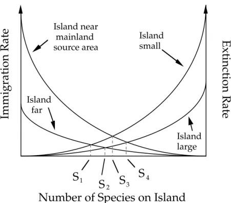
immigration of new species from the mainland and species extinction on the island through demographic drift, even though they did not explicitly interpret their theory as neutral. The two processes are stochastic and their relative frequency determines the number of species found on the island at any given time (cf. Fig. 3). They further assumed that the immigration rate depends on the distance to the mainland, and that the extinction rate depends on the island’s area, thus enabling empirical comparison of their theory to observations (Simberloff & Wilson, 1969).
Figure 3. MacArthur & Wilson (1967) were the first to combine dispersal limitation and demographic drift into a simple model, that aims at explaining the number of species found on islands. They assumed that the number of species results from a dynamic equilibrium between stochastic immigration and extinction, which are dependent on distance to the mainland and on island size, respectively. Adapted from Hubbell (2001).
The theory of island biogeography was later expanded to better account for empirical observations (Brown & Kodric-Brown, 1977). It was also proposed that it might apply more generally to any patch of isolated habitat (Brown, 1978). In parallel, Watterson (1974) and Caswell (1976) used the mathematical tools of population
M a c A R T H U R A N D W I L S O N’ S R A D I C A L T H E O R Y
Fig. 1.3. Various enhancements to the basic equilibrium hypothe-sis of MacArthur and Wilson do not change the dispersal assembly assumption underlying the model. Downwardly bowing immigration and extincton curves were added to characterize the effects of compe-tition on these rates, but all species, whether early or late colonizers, good or bad competitors, experience the same changes in rates. Sim-ilarly, the effects of island distance from the mainland and island size on immigration and extinction rates, respectively, operate equally on all species.
and Wilson fully appreciated the implications of this rad-ical assumption. A majority of their 1967 monograph was devoted to discussing such topics as species ences in colonization strategies, causes of species differ-ences in extinction rates, temporal patterning in the order in which species would successfully establish, and so on—all differences forbidden by their model! Although MacArthur and Wilson (1967) wrote about traditional ecological pro-cesses such as competition, the actual parameters of their model were immigration and extinction rates, distance from
15 genetics to model neutral communities at the level of individual organisms instead of the level of species, thus providing a more mechanistic description of the processes, but without including dispersal limitation. Hubbell (1979, 1997, 2001) eventually combined both ideas into an influential neutral model, which he used as a basis to propose a ‘unified neutral theory of biodiversity and biogeography’. His theory not only states the importance of demographic drift and dispersal limitation for community assembly, but also proposes that they may be the dominating mechanisms in some species-rich communities, especially tropical forest trees and coral reefs. Indeed, strong interspecific competition and predation could act as equalizing mechanisms between species in these communities, as mentioned earlier, and combine with strong intraspecific competition to make all individuals of all species effectively equivalent (Scheffer & van Nes, 2006). Another hypothesis is that in highly diversified communities, complex interspecific interactions could average out at the scale of the community, leading to an ‘emergent neutrality’ (Holt, 2006).
In Hubbell’s model, the mainland’s species reservoir, called the ‘metacommunity’, undergoes a demographic drift where random extinctions are offset by random speciation events. The island, or ‘local community’, also undergoes a demographic drift, but random extinctions are offset by the dispersal, or immigration, of individuals from the source metacommunity. Since the model is neutral, all individuals are considered to have the same dispersal capacity, irrespective of the species they belong to. The scope of the theory is not limited to isolated habitat patches: the local community may represent any spatially delineated ecological community, while the metacommunity represents the regional pool of species constituted by the aggregation of all local communities. The model is controlled by two parameters, the frequency of speciation events in the metacommunity, which determines the regional species richness, and the frequency of immigration into the local community. The immigration flux into the local community modulates its connectivity with the metacommunity: the stronger the immigration flux, the more species-rich and the more similar to the metacommunity the local community is. Hubbell’s model and subsequent related neutral models (Etienne & Alonso, 2007) are amenable to several quantitative
Introduction 16 predictions, and thus to statistical testing (this is discussed in more details in sections II.1 and III.4).
Two distinct neutrality assumptions can be distinguished in Hubbell’s neutral theory: one regarding the metacommunity dynamics, over an evolutionary timescale, and one regarding the local community dynamics, over the timescale of an individual’s lifetime. Predictions regarding local community structure, namely the relationship between area and species richness, the decay of taxonomic similarity with distance, and the distribution of relative species abundances (see section II.1), integrate both assumptions. They are in good qualitative agreement with empirical data (Hubbell, 2001), nevertheless most datasets exhibit quantitative departure from neutrality (McGill et al., 2006). The assumption of a neutral diversification dynamics in the metacommunity can be tested separately, and has been shown to be unrealistic. Indeed, the mean species age predicted by Hubbell’s model are not consistent with empirical measurements (Ricklefs, 2003, 2006), and the shape of the predicted phylogenetic trees does not match that of empirically reconstructed trees (Davies et al., 2011). Hence, recent approaches have instead focused on testing separately the assumption of local neutral assembly through immigration, with contrasting results depending on the system (Sloan et al., 2006; Jabot et al., 2008; Ofiteru et al., 2010; Harris et al., 2015).
Even though comparison of empirical patterns to model predictions suggests that real ecological communities are rarely neutral, Hubbell’s neutral theory retains important merits (Alonso et al., 2006). Indeed, it has been pointed out that all the processes of community ecology are underpinned by only four fundamental processes: natural selection, demographic drift, speciation, and dispersal (Vellend, 2010). Yet, the majority of ecological literature focuses on only one of them, natural selection, which underpins all niche differences between species and thus all deterministic ecological processes. In contrast, Hubbell’s neutral theory focuses on the three remaining fundamental processes, which are inherently stochastic, and places them in a quantitative framework. In practice, neutral models are essential tools for two main uses (Rosindell et al., 2012). Firstly, they may serve as a ‘null model’ against which empirical patterns can be contrasted, so as to identify cases where neutral processes are
17 sufficient to explain the data and cases where they are not. Secondly, they may serve as a parsimonious approximation to real systems, and as a foundation for incorporating relevant non-neutral mechanisms, such as niche differences (Chisholm & Pacala, 2010), environmental stochasticity (Kalyuzhny et al., 2015), negative density-dependence (Du et al., 2011), or a more realistic speciation dynamics (Rosindell et al., 2010). Spatial and temporal scales 4.
Community assembly involves a range of temporal and spatial scales spanning many orders of magnitude - from the evolutionary timescale to the behaviour of individual organisms, and from the global scale to the scale of microorganisms (Chave, 2013). The continental scale is the realm of biogeography, where species distribution reflects the geological and evolutionary history of continents (Cox et al., 2016), as well the latitudinal gradient of diversity (Hillebrand, 2004). At the opposite end, most studies on species interactions focus on a limited number of individuals. Community ecology is concerned with the intermediate scales (Lawton, 1999): namely, within a biogeographic unit (Morrone, 2015), but encompassing a number of individuals large enough for statistical patterns to emerge. The scale at which statistical patterns start emerging depends on the type of organisms considered, and will differ by many orders of magnitude between plants and bacteria.
Niche and neutral processes might alternately dominate at different spatial and temporal scales. Firstly, locally observed species interactions do not preclude random species assembly over larger spatial and temporal scales. Indeed, the majority of interspecific interactions are opportunistic and vary across space and time (Holt, 1996; Poisot et al., 2014), despite much-studied instances of specialized interspecific interactions such as plant-pollinator mutualisms (Rønsted et al., 2005). Secondly, species dynamically adapt their niche to the local competitive context, either through plasticity or through natural selection. For instance, closely related species with mostly disjoint geographical distributions are known to display greater phenotypic differences
Introduction
18
(such as a difference in size) wherever they co-occur, a process known as ‘character displacement’ (Brown & Wilson, 1956). Natural selection has been found to have measureable effects on phenotype over timescales as short as a few generations when species are confronted with a sudden change in their biotic or abiotic environment, thus questioning the legitimacy of the traditional separation between the timescales of evolutionary and community assembly processes (Ghalambor et al., 2015).
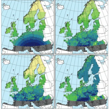
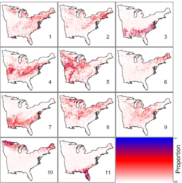
Figure 4. Community assembly processes depend on the spatial and temporal scales considered: current geographical patterns of tree diversity in Europe might reflect on-going dispersal from ice age tree refugia, which started 14,000 years ago. Top right, bottom left and bottom right: geographical distribution of tree diversity (increasing from yellow to blue) for all 60 European tree species, the 45 temperate species and the 15 boreal species, respectively. Top left: accessibility through dispersal from ice age tree refugia (black dots). Adapted from Svenning & Skov (2007).
Another key aspect of community assembly is how fast community composition responds to abiotic change, relative to the pace of the abiotic change itself. Indeed, if abiotic change is fast enough relative to community response, the community may never reach equilibrium, thus leading to an apparently random dynamics. This
present time, i.e. extrinsic ecogeographical factors. Notably, it is easy to imagine that the cold-hardy Quercus robur had more and more northerly located refugia than Q. cerris and for this reason could achieve an earlier and faster postglacial spread. The first tree species to spread would have met much less competition from other tree species than late-spreading species, which would have had to spread through well-established late-successional forest communities. Sven-ning & Skov (2004) did in fact find a relatively strong positive correlation between range filling and cold hardiness in European trees.
C A N C U R R E N T P A T T E R N S O F T R E E D I V E R S I T Y B E P R E D I C T E D F R O M A S I M P L E M E A S U R E O F
A C C E S S I B I L I T Y F R O M G L A C I A L R E F U G I A ?
While it is evident that climate and to a lesser extent other environmental factors such as soil do constrain Europe-wide tree species diversity and distribution patterns (Walter & Breckle 1986; Pigott 1991; Sykes et al. 1996; Svenning &
Skov 2005), we will now consider the extent to which these patterns could entirely be caused by dispersal.
If diversity patterns were entirely driven by limited dispersal out of the glacial refugia, we expect that the areas that are most accessible from the refugia, i.e. located closest to the greatest number of refugia, would harbour the greatest number of species. Figure 2 shows the pattern of accessi-bility across Central and Northern Europe as well as the observed pattern of tree species richness. The accessibility (ACC) of each grid cell in the receiving area (Central and Northern Europe) was computed as the inverse of the summed distances to all grid cells in the source area. Hence, the more distant a receiving grid cell on average is located from any one source cell the lower its accessibility. The source area was set to be Southern Europe at 43–46! N, as postglacial expansions into Central and Northern Europe primarily took place from or via this region (e.g. Petit et al. 2002; Magri et al. 2006). Albeit some of the most cold-tolerant tree species had LGM refugia somewhat further north, especially in eastern Europe (Willis & van Andel
Figure 2 Top-left: The accessibility of each 50· 50 m grid cell in Central and Northern Europe to postglacial immigration from the ice age tree refugia, computed as the inverse of the summed distances to all grid cell in the source area (Southern Europe at 43–46! N). Top-right: The current native species richness of tree species (60 species in total, 2–31 species per cell) in Europe. Right: Bottom-left: The current native species richness of temperate tree species (45 species in total, 0–22 species per cell). Bottom-right: The current native species richness of boreal tree species (15 species in total, 0–10 species per cell). Colour coding corresponds to 10 equal frequency categories, with yellow over green to blue representing low to high accessibility and few to many species, respectively.
456 J.-C. Svenning and F. Skov Idea and Perspective
19 phenomenon may be more pervasive than it seems: for instance, it has been shown that the dispersal of tree species in Europe following the end of the last ice age is still an on-going process (cf. Fig. 4; Svenning & Skov, 2007). In contrast, organisms with short generation time and high dispersal ability are able to track environmental changes more efficiently. Additionally, if several local communities are connected by a permanent and strong enough dispersal flux, they may never reach the optimal composition that would be expected based on local abiotic conditions (Gravel et al., 2006). A local community will also be more prone to demographic stochasticity if it hosts a smaller population size (Fisher & Mehta, 2014). These observations have led to the development in the last decade of ‘metacommunity theory’, a family of mathematical models aiming at reconciling neutral and niche processes by explicitly accounting for spatial and temporal dynamics (Leibold et al., 2004). However, unlike simpler neutral models, these models do not provide predictions that are easily amenable to statistical comparison with empirical data.
Lastly, most of the existing knowledge on community assembly comes from the study of plants and vertebrates, and the extension of community ecology to microorganisms is comparatively very recent (Curtis & Sloan, 2005; Martiny et al., 2006; see section II.2). While the fundamental processes of community assembly apply to all living organisms, they operate over very different scales for microorganisms, and their relative importance is likely to differ (Hanson et al., 2012). It has long been considered that microorganisms had effectively infinite dispersal capacity, and that abiotic filtering was the dominant process of community assembly (Baas Becking, 1934). Microbial communities have indeed been found to be very sensitive to local abiotic conditions and dominated by specialist taxa (Ramirez et al., 2014; Mariadassou
et al., 2015). Nevertheless, this view has now been nuanced, and dispersal limitation has
been shown to play a role as well (Ofiteru et al., 2010; Martiny et al., 2011; Roguet et al., 2015). While microorganisms tend to be more cosmopolitan than larger organisms, biogeographic patterns do exist (Hanson et al., 2012; Livermore & Jones, 2015). Microorganisms have also been found able of complex interactions beyond competition (Cordero et al., 2012).
Introduction 20
21
II. DNA-based biodiversity patterns
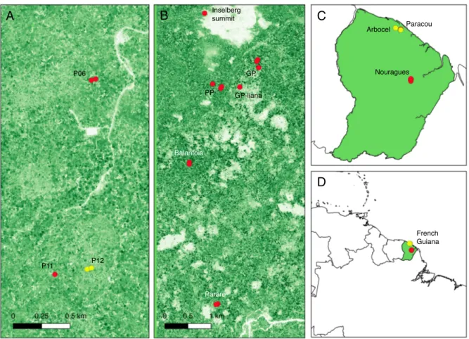
Most of ecological knowledge comes from studies performed at the level of individual species, and from this perspective, the singularity of each species and sometimes of each individual is striking. Thus, ecologists have long wondered whether general laws were hiding behind the collection of idiosyncrasies (Lawton, 1999). Integrative data on species richness, abundance and spatial occurrence have been gathered with the hope that they would yield insight into the general mechanisms of community assembly (Brown, 1995). The underlying idea is that, as in statistical physics, informative statistical properties might emerge from the observation of a large enough number of individuals and species irrespective of the details of species identities.In this section, I first introduce two types of integrative patterns that have been widely studied in community ecology: the distribution of species abundances, and spatial patterns. I then discuss why the emergence of automated data collection is opening new horizons for the study of these patterns. Lastly, I briefly present the ecosystem that this thesis more specifically focuses on, the tropical forests of French Guiana. Integrative biodiversity patterns 1. a. Species relative abundances
The distribution of species abundances in a random sample of individuals takes two forms in the ecological literature: the ‘rank-abundance distribution’ (RAD), or ‘Whittaker’s plot’, consists of the abundances ni of all S species in the sample ranked by
Introduction
22
plot’, is the distribution of the number Φ! of species having abundance n for all the possible n values in 𝑛!, … , 𝑛! (cf. Fig. 5; Preston, 1948; Whittaker, 1965). To
accommodate the limited amount of data, the SAD is usually binned into abundance categories. This binning step leads to a loss of information, thus the RAD is more informative than the SAD. Nevertheless, the SAD has often been the preferred distribution because it is easier to handle mathematically and to derive from theoretical models. This is linked to the fact that it can be interpreted upon normalization as the probability distribution for the abundance of a randomly chosen species in the sample. Because of the wide range of abundances typically observed in empirical data, abundances are often log-transformed in SAD and RAD – in SAD, this amounts to binning species into abundance classes of exponentially increasing width from the lowest abundance class (one individual) to the highest, following the example of Preston (1948).
It was noticed early on that the distribution of species abundances tended to be similar in species-rich communities. Indeed, within a single trophic level, there are usually a few common species and a long tail of rare species – simply put, ‘most species are rare’ (cf. Fig. 5). This spurred attempts at finding a general explanation for this pattern. Fisher et al. (1943) and Preston (1948) were the first to propose statistical distributions to fit the distribution of species abundances.
Fisher assumed that the sampled species abundances followed a negative-binomial distribution without the zero-abundance class, and derived a SAD of the form 𝔼 Φ! = 𝛼𝑥! 𝑛, where α is a constant parameter, 𝑥 is a function of α and of sample size
N (with 0 < 𝑥 < 1), and 𝔼 Φ! is the statistically expected value of Φ! (cf. section III.3.b;
Chave, 2004). Since !!!!𝔼 Φ! = −𝛼 ln(1 − 𝑥), this distribution is called the
‘log-series’. A remarkable property of this model is that the expected number of species 𝔼 𝑆 in the sample is given as a function of the number of sampled individuals N by 𝔼 𝑆 = 𝛼 ln(1 + 𝑁 𝛼). Hence, the parameter 𝛼 is sufficient to predict the observed species richness as a function of the sampling effort. It can thus be used as a sampling-independent measure of the community’s diversity. The value of 𝛼 can be easily
23 visualized in the RAD representation, since the log-transformed abundances are expected to decrease linearly with slope −1 𝛼 as a function of species rank (cf. Fig. 5).
Preston (1948) argued in contrast that a log-normal SAD best fitted empirical data, i.e. 𝔼 Φ! ∝ 𝑒! !" !!! !!! with 𝜇 and 𝜎 constant parameters. A notable difference
between the two SADs is that the log-normal distribution exhibits a mode (i.e., the abundance class with the most species is not the lowest abundance class), while Fisher’s log-series does not. Preston explained the fact that both situations could be encountered in empirical data by the effect of sampling: a community in which the ‘true’ SAD (i.e., for
M E T A C O M M U N I T Y D Y N A M I C S
Fig. 5.7. Preston-type plot of relative species abundance for tree species >10 cm dbh in the 50 ha BCI plot, compared with expecta-tions from the lognormal, and from the zero-sum multinomial of the unified neutral theory, for θ = 50 and m = 0"10. The error bars are ±1 standard deviation.
Fig. 5.8. Preston-type plot of relative species abundance for tree species >10 cm dbh in the 50 ha Pasoh plot, compared with expecta-tions from the lognormal, and from the zero-sum multinomial of the unified neutral theory, for θ = 180 and m = 0"15. The error bars are ±1 standard deviation.
135
M E T A C O M M U N I T Y D Y N A M I C S
Fig. 5.9. Fitted and observed dominance-diversity distributions for trees >10 cm dbh in the 50 ha plot on Barro Colorado Island, Panama. The best fit θ had a value of 50. Note the departure of the metacom-munity distribution for very rare species, but that the observed distri-bution is fit well once dispersal limitation (m = 0"10) is taken into account. The error bars are ±1 standard deviation.
each figure. The metacommunity logseries distribution is the diagonal line extending downward beyond the empirical curves to the lower right. The metacommunity distribution was calculated for a fitted θ value of 50 in the case of the BCI forest, and for a fitted θ value of 180 in the Pasoh for-est. Then the parameters for dispersal limitation and local community size were included to predict the local commu-nity dominance-diversity curves in each forest plot. Local community size was 20,541 trees > 10 cm dbh in the BCI plot, but it was 28% higher (26,331) in the Pasoh plot. The previously estimated values of m of 0.10 and 0.15 for BCI and Pasoh, respectively, were used. The precision of the predicted local dominance-diversity curves in each plot is readily apparent from figures 5.9 and 5.10. The expected distributions fit even the abundances of the rarest species
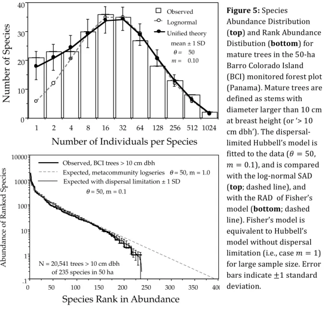
137 Figure 5: Species Abundance Distribution (top) and Rank Abundance Distibution (bottom) for mature trees in the 50-ha Barro Colorado Island (BCI) monitored forest plot (Panama). Mature trees are defined as stems with diameter larger than 10 cm at breast height (or ‘> 10 cm dbh’). The dispersal-limited Hubbell’s model is fitted to the data (𝜃 = 50, 𝑚 = 0.1), and is compared with the log-normal SAD (top; dashed line), and with the RAD of Fisher’s model (bottom; dashed line). Fisher’s model is equivalent to Hubbell’s model without dispersal limitation (i.e., case 𝑚 = 1) for large sample size. Error bars indicate ±1 standard deviation.
Introduction 24 an infinite number of individuals) is log-normal can lose its mode if under-sampled, and be mistaken for a log-series. It has since then been acknowledged that the effect of sampling is indeed paramount in our ability to distinguish between differently-shaped SAD by curve-fitting (Sloan et al., 2007). In the RAD representation with log-transformed abundances, a log-normal SAD takes the form of an S-shaped curve, the common species being commoner and the rare species rarer than in Fisher’s log-series.
Later models have focused on finding a mechanistic justification for the proposed distributions. MacArthur (1957) proposed that species relative abundances resulted from the random partitioning of the niche space between the different species of the community. A number of more sophisticated niche partitioning models’ were subsequently proposed (Tokeshi, 1996; McGill et al., 2007). However, Hubbell’s neutral model is the mechanistic model that has been the most successful at fitting empirical SADs (Hubbell, 2001; cf. section I.3 and III.4). Indeed, the metacommunity SAD converges toward Fisher’s log-series for a large enough sample size and is characterized by a ‘fundamental biodiversity number’ θ that converges toward Fisher’s 𝛼 (Chave, 2004). In the absence of dispersal limitation, the local community is a random sample from the regional metacommunity, and hence also exhibits a log-series-like SAD. In the presence of dispersal limitation however, the depletion of rare species and the increase in abundance of locally common species lead to a log-normal-like SAD (cf. Fig. 5). Thus, Hubbell’s neutral model can approximate both the log-series and the log-normal SADs, while providing a mechanistic justification for them and fully accounting for sampling effects. Nevertheless, it has been shown that many types of non-neutral processes could yield SADs similar to neutral ones (Chave et al., 2002; Pueyo et al., 2007; Chisholm & Pacala, 2010). It has also been argued that the log-normal distribution fits empirical SADs at least as well as Hubbell’s local community SAD (McGill, 2003). The log-normal is still the most popular choice when it comes to choosing a realistically-shaped SAD for modelling purposes irrespective of the underlying mechanisms (Connolly et al., 2017). A log-normal SAD is not in itself very informative on the mechanisms of community assembly. Indeed, the log-normal distribution is the limiting probability distribution for
25 any product of sufficiently many random variables, as a consequence of the central limit theorem (cf. section III.2 and III.3.a), thus a log-normal SAD could arise as the result of any type of multiplicative process. More generally, it has been suggested that the range of empirically observed SADs could simply result from the iterative spatial aggregation of smaller-scale SADs, a phenomenon described as a ‘spatial analogy of central limit theorem’ (Sizling et al., 2009). As a consequence, it has been called for, on the one hand, more statistically powerful tests than simple curve-fitting (Chave et al., 2006; Al Hammal et al., 2015), and on the other hand, testing multiple predicted patterns simultaneously instead of solely the SAD (McGill et al., 2007).
b. Spatial patterns
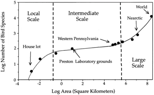
Spatial patterns form a second family of integrative patterns in ecology. The relationship between the sampled area and the number of sampled species is the oldest such pattern to have been studied (Watson, 1859). This curve was first regarded as a mean to assess whether a community had been adequately sampled, i.e. to ensure that only a marginal number of new species would appear in the sample if the sampled area were to be increased. It was soon realized that the species-area relationship (SAR) might also contain valuable information regarding spatial community structure. Indeed, at the regional scale, the number of species S was found to consistently follow a power law 𝑆 ∝ 𝐴! as a function of area A, where the exponent z takes values between 0.15 and
0.40 (Arrhenius, 1921; Williamson, 1988). This ‘law’ has later been observed to break down at the extremes, either for areas that are below approximately 1 km2 (for plants or vertebrates), or conversely for areas that exceed the boundaries of a single biogeographic unit (cf. Fig. 6; Preston, 1960; Shmida & Wilson, 1985). The resulting curve exhibits an ‘S’ shape on a log-log scale, with a linear domain in the central part corresponding to the power-law behaviour described above, and steeper slopes at both ends.