Wavelet transform: A tool for the interpretation of upper mantle converted phases at high frequency

HAL Id: hal-01767215

https://hal.archives-ouvertes.fr/hal-01767215

Submitted on 16 Apr 2018

HAL is a multi-disciplinary open access

archive for the deposit and dissemination of

sci-entific research documents, whether they are

pub-lished or not. The documents may come from

teaching and research institutions in France or

abroad, or from public or private research centers.

L’archive ouverte pluridisciplinaire HAL, est

destinée au dépôt et à la diffusion de documents

scientifiques de niveau recherche, publiés ou non,

émanant des établissements d’enseignement et de

recherche français ou étrangers, des laboratoires

publics ou privés.

Wavelet transform: A tool for the interpretation of

upper mantle converted phases at high frequency

Julie Castillo, Antoine Mocquet, Ginette Saracco

To cite this version:

Julie Castillo, Antoine Mocquet, Ginette Saracco. Wavelet transform: A tool for the

interpreta-tion of upper mantle converted phases at high frequency. Geophysical Research Letters, American

Geophysical Union, 2001, 28 (22), pp.4327-4330. �10.1029/2001GL013214�. �hal-01767215�

GEOPHYSICAL RESEARCH LETTERS, VOL. 28, NO. 22, PAGES 4327-4330, NOVEMBER 15, 2001

Wavelet transform ß A tool for the interpretation

of upper mantle converted phases at high frequency

Julie Castillo, Antoine Mocquet,

Laboratoire de Plan•tologie et G•odynamique, Nantes University, France.

Ginette Satacco 1

Laboratoire de G•osciences, Rennes University, France.

Abstract. P to S converted receiver functions recorded at

VBB FDSN California stations are studied in the frequency range of 0.1 to i Hz. Microseismic noise is maximum in this frequency range, but signal processing by the wavelet

transform enables us: (1) to enhance seismic phases asso-

ciated with seismic velocity gradients and discontinuities at

the base of the upper mantle, (2) to extract accurate ar- rival times, and (3) to obtain an accurate insight into the

frequency content. In the case of California, one seismic

discontinuity and two zones of high gradients in the depth

range of 625 to 720km are recurrently observed for two dif-

ferent data sets.

Introduction

Many studies have focused on the interface between the upper and the lower mantle of the convective Earth. The diversity of seismic phases and frequency ranges used for the interpretation has lead to the construction of different mod- els. The most commonly used model consists of a less than

5-km thick discontinuity

(e.g. Paulssen

[1985]) which is sit-

models, hereafter abbreviated as SSEM (e.g. ak135, [Ken-

nett et al., 1995]). Mineral physics

indicates

that the depth

endothermic transformation of ringwoodite (•-phase) into

perovskite (Pv) and magnesiowustite

(Mw) (e.g. Ito and

Takahashi

[1989]). Studies also predict the presence

of high

formation of non-olivine minerals (i.e. garnet and ilmenite)

[Vacher et al., 1998]. These results

support the opinion that

contrast associated with the transformation of non-olivine

components is predicted to be 6 times smaller than the one associated with the transformation of olivine phases, ob-

servations

by Niu and Kawakatsu [1996] under Japan and

China, and Simmons and Gurrola [2000] under California,

Now at Laboratoire Cerege, Aix-Marseille, France.

Copyright 2001 by the American Geophysical Union. Paper number 2001GL013214.

0094-8276/01/2001GL013214505.00

by seismological means. Since the amplitude of a converted phase depends on the ratio between the width of the in- terface and the wavelength, the frequency content of dis- persed waveforms provides information on the smoothness of seismic discontinuities. High seismic gradients related to non-olivine transformations are 10 to 50km thick; thus, P to

S converted

phases (Pds) should be studied at frequencies

move this noise (see [Chevrot et al., 1999] for a review), but

they exhibit a radial resolution worse than 30km. In this paper, we apply the wavelet transform to high frequency

(0.1-1Hz) deconvolved Pds Very Broad Band (VBB) wave-

forms. This data processing technique, which has been used

in various

geophysical

fields (e.g., [Paulssen,

1985; Kumar et

al., 1997; Moreau et al., 1999; Valero, 2000]), makes it possi-

ble for us: (1) to detect accurately

the arrival time of seismic

phases

converted

at sharp (less than 10km thick) disconti-

nuities (2) to highlight waveforms generated through high

seismic gradients and derive their frequency content, and

consequently (3) to improve the radial resolution of seismic

models close to the 660km depth range. The efficiency of the method is discussed using VBB data recorded at 3 FDSN

California stations.

Data processing

We convolve the discrete complex Morlet wavelet (e.g.

Morlet et al., [1982]) with the studied signal, in the fre-

complementary

information: high values (rr > 1) provide a

ues favor the accurate detection of arrival times. An initial

data set of 138 three-component seismograms generated be- tween 1991 and 1996 in the Tonga subduction zone - in the magnitude range of 5.5 to 7, and depth ranges of 0-70km and 400-680km - has been constructed with epicentral distances contained between 65 and 85deg. for the 3 stations under

study (figure la). Only events displaying a signal to noise

(S/N) ratio greater than 10 for the P-wave arrival on the

by azimuthal anisotropy [Montagner, 1998] are reduced by

4328 CASTILLO ET AL.- RECEIVER FUNCTION ANALYSIS WITH WAVELET TRANSFORM go be

•

-0.09

•

-0.11

•-0.13

•-0.15

•

-0.17

time before P-wave arrival (sec)

Figure 1. (a) Stations (triangles) and events used in this study. Black circles: deep events (hypocenter depth greater than 450km); white circles: shallow events (hypocenter depth smaller than 70km). (b) Stacked receiver functions as a function of slow-

ness. Slowness values are relative to the one of the direct P-wave.

nent traces. Two subsets are constructed in order to detect

possible artifacts induced by heterogeneities in the source region, and to test the redundancy of the interpretation in

terms of mantle structure. The subsets consist of 34 shal-

low events

(focal depth h shallower

than 70km), and 18 deep

events

(h _> 400km), respectively.

The stacked

receiver

func-

tions are obtained using Vinnik's [1977] method for a refer-

ence distance of 75deg. The time window of the deconvolv- ing P-wave is tested in the range 10 to 40s. The slowness

values of the normal move-out corrections are tested in the

range

(-0.09,-0.17) s.deg

-• (figure

lb). Figure

3 is focused

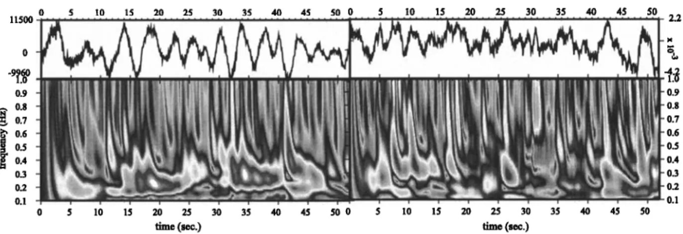
on P to S conversions at 660km depth. Between 53 and 75sec, the maximum error on arrival times is lower than +0.3sec. The energy level of the post-stack noise sampled before the P-wave arrival is illustrated in figure 2. In the frequency range 0.1-1.0Hz, the noise energy level is domi-

nated by the coherent microseismic noise at 0.25Hz (figure

2a). Deconvolution

and stacking

serve to increase

the S/N

frequency range (figure 2b). The S/N ratio is close to 2.5 for

the stack of the 52 SV-components, while it is lower than 0.5 for individual traces. This effect is important for further signal interpretation, since 0.2-0.4Hz is the frequency range in which waves generated on upper mantle seismic gradients are expected to reach maximum energy.

Results

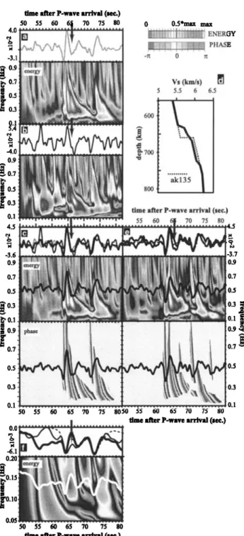
The stacked deconvolved Pds traces are shown in figures 3a and 3b, respectively for deep and shallow events. Sev- eral packets stand out of the time frequency energy dia- gram. The features common to both stacks are described first. The energy maximum arrives with a time lag of +3s with respect to the P660s arrival time predicted by ak135.

Two additional maxima are observed between 0.3 and 0.5Hz.

The arrival times of the latter are around 66s, and 73s, re- spectively. Among the three successive arrivals, only the second one displays a significant dispersion over a 4s wide time window, indicating a 20km thick structure. The first and third phases are sharp and non-dispersive. This sug- gests that they were generated on discontinuities. On the

shallow events stack (figure 3a) these arrivals dominate the

(figure 3b), a fourth high energy arrival is observed around

57s. It is slightly dispersed over a 3s wide window, and its frequency content is maximal around 0.3 Hz, similar to

the arrival around 65s. If we consider that the remainder

of the seismogram corresponds to noise, the energy ratio of the four arrivals with respect to the maximal noise level is equal to 1.6 at 0.3Hz, 1.6 at 0.55Hz, 2 at 0.33Hz, and 1.2 0 5 10 15 11500 0

'1•.•

o

0.9

•

•ø'5

i

•.•••

...

'•"'"'

.'-"..•:'•• • ;...•_.

• ...

•0•1•.•

.•....

:•••.•:....••,•••,---'--•.

---•z-':--••

0.2

m ...

"':':•::•'

---74'•'":-••;'•-•

'•

o.1

Figure 2. Effect of deconvolution on random and coherent noise. Energy diagrams of stack of seismograms recorded on the 52 invidual SV components before P-wave arrival (a) before and (b) after deconvolution. The corresponding energy scale bar is displayed

CASTILLO ET AL- RECEIVER FUNCTION ANALYSIS WITH WAVELET TRANSFORM 4329

time after P-wave arrival (sec.)

50 55 60 6• 70 75 80 40 ... -3.11 • /

... -

...

:':

energy

L._{:;?

•J•

[ :'""'=:::'::'•:::":';:;'

•0.7

0.7

•&:ii:½•--.:½-.:.:,-..,;;i•ii•[: •:i;:.'l:-"""•½.,.&:,,, PHASE

-:n 0 6O0

•700

v, 0•,)

•

time after P-wave arrival (sec.)

55 60 70 75 80 ,4.5 -37 0.9 0.7 0.5

o.3

0.9

•

•0.15

time after P-wave arrival (sec.)

50 55 60 65 70 75 80

time after P-wave arrival (sec.)

0.3

O. 1

Figure 3. Wavelet transform of Californian Pds VBB records.

Arrows point at the P660s phase predicted by ak135. For sake of clarity, phases are displayed only if the energy is greater than one third of the maximum energy. Amplitudes are normalized

with respect to the amplitude of the P-wave. (a) 34 shallow events stack; (b) 18 deep events stack; (c) total stack (heavy solid curve). (d) Shear wave velocity profile accounting the best for the observations. (e) thin curves correspond to synthetic seis- mograms without (dashed curve) and with (solid curve) noise, the heavy solid curve corresponds to the total stack of figure (c); the

phase and energy diagrams correspond to the synthetic seismo-

gram. (f) total stack (heavy solid line) and noisy synthetic seis- mogram (thin line) filtered with a 0.167 lowpass; the phase and

energy diagrams belong to the total stack. A colored version of

this figure is available on the website: http://www.sciences.univ- nantes.fr/geol/UMR6112/Persnl/JCastillo/castillo.html

at 0.6Hz. These values confirm that the deep events stack

is noisier than the shallow events one. Interference between

noise and converted waveforms could be responsible for the differences in energy ratios between the different phases ob- served on each stack The low energy ratios of the deep

events stack make it difficult to discriminate between two

interpretations: either the 57s, and the 66s arrivals cor- respond to converted phases on mantle interfaces, or the energy diagram is dominated by noise. Similarities in both

stacks (figures 3a and 3b) lead one to believe that the 66s

the best fit between the observations and WKBJ seismo-

grams [Chapman,

1978] in the frequency

interval 0.1-1Hz is

2b with a S[N ratio of 2, and filtered in the frequency range

0.1-1Hz. Several stacks have been produced by delaying the noise track with respect to the bare synthetic seismogram. Though we have chosen the combination that fits the best with the observations, the interference between converted phases and noise results in slightly shifting their frequency

content. This effect contributes to the error on the values of

interfaces' depths and thickness by the order of 4- lkm.

Discussion

Dispersed waveforms generated on seismic gradients be- come dominant at long period, and they may hide the pres- ence of sharp discontinuities, especially if both structures are in close proximity to one another. In fact, geodynamical interpretation based on low frequency signals, and on the assumption of a single discontinuity at the base of the up- per mantle can be biased by the inadequacy between signal- wavelength and investigated structure thickness. A 0.167Hz

low-passed

version

of the total stack and its synthetics

(fig-

ure 3f) shows that the three phases previously identified at

higher frequencies

(figure 3c) are more difficult--to

discrimi

....

4330

CASTILLO ET AL.: RECEIVER FUNCTION ANALYSIS

WITH WAVELET TRANSFORM

pled interfaces. A combined use of standard deconvolution

techniques

and the wavelet

transform

allows

the seismic

sig-

nal to stand out from noise, and individualize arrival times of sharp phases generated on seismic discontinuities from

dispersed

waveforms

created

by gradients. The high fre-

quency

(0.1-1Hz)

results

obtained

in the present

study

yield

the relative depth and thickness of these structures with a better accuracy than lowpassed waveforms. Under Cali-

fornia, we find a seismic

structure

which is more complex

than usually

observed

by studies

based

on long-period

data

(e.g. Shearer

and Flanagan

[1999]. Our results

are con-

sistent with the larger scale observations of Simmons and

Gurrola [2000] in the same region, i.e. the three interfaces

located

at 625, 650, and 720km depth, respectively.

Our

model can be viewed as a lateral average

of their detailed

three dimensional

map of the transition zone beneath Cal-

ifornia. The main difference between both studies lies in

the visibility of the 625km discontinuity,

which is enhanced

in our model while it is not present everywhere

on a re-

gional scale. We suspect the link between seismic interfaces

and mineralogical

transformations,

as predicted

in the lab-

oratory, is not straightforward. For example, we obtain a

thickness

of about 20km for the 650km interface,

while ex-

perimental

studies

[Ito and Takahashi.,

1989] predict that

the transformation

of ringwoodite

occurs

over a region

less

than 5km thick. The 625km discontinuity

may also be a

good

candidate

for this reaction

since

Irifune et al. [1998]

have reported

that it could take place at mantle pressures

valid at a depth of 600km. On the other hand the 720km

deep structure

can be attributed more confidently

to the

transformation

of ilmenite into perovskite,

if one considers

the depth range in which this transformation

is likely to

occur (e.g. Vacher

et al. [1998]). The method

which has

been applied here proves itself to be a useful method for

further observations

in different

geodynamical

contexts

and

comparison with laboratory results.

Acknowledgments.

This work

was financed

by French

MRT, and by IT program of INSU. We acknowledge the IRIS team for providing the data and Scherbaurn and Johnson for the PITSA toolkit. Figures have been designed with the GMT toolkit of Wessel and Smith, [1991]. Constructive comments by Pierre

Vacher,

Scott

Turner

and an anonymous

reviewer

have

been

help-

ful to improve a first version of this paper. References

Chapman, C.H., A new method for computing synthetic seismo- grams, Geophys. J. R. astr. Soc., 54, 481-518, 1978.

Chevrot, S., Vinnik, L., and J.-P. Montagner, Global patterns of upper mantle from Ps converted waves, J. Geophys. Res., 104, 20203-20219, 1999.

Irifune, T. N. Nishiyama,

K. Kuroda, T. Inoue, M. Isshiki,

W.

Utsumi,

K. Funakoshi,

S. Urakawa,

T. Uchida,

T. Katsura,

and O. Ohtaka, The postspinel phase boundary in Mg2SiO4

determined

by in-situ X-ray diffraction,

Science,

279, 1698-

1700, 1998.

Ito, E., and E.Takahashi.,

Postspinel

transformations

in the sys-

tem Mg2SiO4-Fe2SiO4 and some geophysical implications, J.

Geophys. Res., 94, 10,637-610,646, 1989.

Kennett, B.L.N., E.R. Engdahl, and R. Buland, Constraints on seismic velocities in the Earth from traveltimes, Geophy. J.

Int., 122, 108-124, 1995.

Kumar, P., and E. Foufoula-Georgiou,

Wavelet

analysis

of geo-

physical applications, Rev. Geophys., 35, 385-412, 1997. Montagner J.-P., Where can Seismic Anisotropy be detected in

the Earth's Mantle? In Boundary

Layers...,

Pageoph.,

151,

223-256, 1998.

Moreau,

F., D. Gibert, M. Holschneider,

and G Saracco,

Identifi-

cation of sources of potential fields with the continuous wavelet

transform:

i- Basic

theory,

J. Geophys.

Res., 104, 5003-5013,

1999.

Morlet J., G. Arens,

E. Fourgeau,

and D. Girard,

Wave

propaga-

tion and sampling theory, Parts i an 2, Geophysics 47, 203-236,

1982.

Niu, F., and H. Kawakatsu, Complex structure of the mantle

discontinuities at the tip of the subducting slab beneath the Northeast China: a preliminary investigation of broadband

receiver functions, J. Phys. Earth, 44, 701-711, 1996. Paulssen, H., Upper mantle converted waves beneath the NARS

array, Geophys. Res. Lett., 12, 709-712, 1985.

Shearer,

P.M., and M.P. Flanagan,

Seismic

velocity

and density

jumps across the 410- and 660-kilometer discontinuities, Sci- ence, 285, 1545-1548, 1999.

Simmons, N.A., and H. Gurrola, Multiple seismic discontinuities near the base of the transition zone in the Earth's mantle,

Nature, 405, 559-562, 2000.

Vacher, P., A. Mocquet, and C. Sotin, Computation of seismic

profiles from mineral physics : the importance of the non-

olivine components for explaining the 660 km depth disconti- nuity, Phys. Earth Planet. Inter., 106, 275-298, 1998.

Valdro,

H.-P., Endoscopie

sismique,

PhD thesis,

256 pp., Institut

de Physique du Globe at Paris France, 2000.

Vinnik, L.P., Detection of waves converted from P to SV in the

mantle, Phys. Earth Planet. Inter., 15, 39-45, 1977.

J. Castillo and A. Mocquet,

Laboratoire

de Plandtologie

et

niques,

2, rue de la Houssiniere,

44300

Nantes,

FRANCE (e-mail:

G. Saracco,

Laboratoire

de G•osciences

Rennes,

UPR 4661,

Campus

de Beaulieu,

263 av. du Gdn•ral

Leclerc,

35042

Rennes,

FRANCE

(Received

March

22, 2001; revised

August

04, 2001;