Effect of Slice Thickness on Texture-Based Classification of Liver Dynamic CT Scans

HAL Id: hal-01496055

https://hal.inria.fr/hal-01496055

Submitted on 27 Mar 2017

HAL is a multi-disciplinary open access

archive for the deposit and dissemination of

sci-entific research documents, whether they are

pub-lished or not. The documents may come from

teaching and research institutions in France or

abroad, or from public or private research centers.

L’archive ouverte pluridisciplinaire HAL, est

destinée au dépôt et à la diffusion de documents

scientifiques de niveau recherche, publiés ou non,

émanant des établissements d’enseignement et de

recherche français ou étrangers, des laboratoires

publics ou privés.

Distributed under a Creative Commons Attribution| 4.0 International License

Effect of Slice Thickness on Texture-Based Classification

of Liver Dynamic CT Scans

Dorota Duda, Marek Kretowski, Johanne Bezy-Wendling

To cite this version:

Dorota Duda, Marek Kretowski, Johanne Bezy-Wendling. Effect of Slice Thickness on Texture-Based

Classification of Liver Dynamic CT Scans. 12th International Conference on Information Systems and

Industrial Management (CISIM), Sep 2013, Krakow, Poland. pp.96-107,

�10.1007/978-3-642-40925-7_10�. �hal-01496055�

Classification of Liver Dynamic CT Scans

1

Faculty of Computer Science, Bialystok University of Technology Wiejska 45a, 15-351 Bia lystok, Poland

2

INSERM, U1099, Rennes, F-35000, France

3_{University of Rennes 1, LTSI, Rennes, F-35000, France}

e-mail:{d.duda,m.kretowski}@pb.edu.pl

Abstract. This paper assesses the impact of slice thickness on texture

parameters. Experiments are performed on liver dynamic CT scans, with two slice thicknesses. Three acquisition moments are considered: without contrast, in arterial and in portal phase. In total, 155 texture parame-ters, extracted with 9 methods, are tested. Classification of normal and cirrhotic liver is performed using a boosting algorithm. Experiments re-veal that slice thickness does not considerably influence the stability of the parameters. They also enable to assess the rate of parameter de-pendency on slice thickness. Finally, they show that applying different slice thicknesses for training and testing the CAD system requires slice thickness-independent parameters.

Keywords: texture analysis, classification, dynamic CT, liver, slice thickness,

stability of the parameters, tissue characterization, CAD.

1

Introduction

Various medical imaging techniques are available for acquiring a diagnostic in-formation, e.g., Computed Tomography (CT), Positron Emission Tomography (PET), ultrasound, Medical Resonance Imaging (MRI), Single Photon Emission Computed Tomography (SPECT). With their rapid development, the image quality has been significantly improved. The images acquired over the years are characterized by increasing spatial and grey level resolution, and decreasing slice thickness. The number of images obtained within a single examination increases. The appropriate interpretation of an image information is thus a very complex task, but decisive for a correct diagnosis and treatment proposal.

Due to the fact, that the men are not able to identify such huge amount of in-formation stored in the images, the (semi)automatic Computer Aided Diagnosis (CAD) systems become of a rapidly growing interest. Combining different image analysis techniques (like texture analysis [1] or segmentation) and classification algorithms, they appear to be a very promising diagnostic tool.

In most of the CAD systems based on imaging data two main stages of work can be distinguished. The first one, called training, is a preparation of the system

for the recognition of several classes of tissue, representing different pathologies. The second stage is the applicationof the system for the (semi)automatic recog-nition of new cases, not yet diagnosed. Due to the constant changes of image ac-quisition protocols, the question arises whether the protocols for new recognized images can be different from those that were used during the system training. The question seems all the more important given the fact that there is still no universal consensus on image acquisition protocols, so the images obtained from different machines could be of different properties and qualities.

The aim of our study is to examine the effect of slice thickness on texture parameters characterizing hepatic tissue on dynamic (contrast-enhanced) CT images. Our choice was dictated by the fact that the image database that we have been creating for about 10 years includes images of several slice thicknesses: from the oldest ones, of 10 mm, to the most recent ones, of 1.3 mm. So far, we have not found any research concerning the impact of slice thickness on texture-based classification of liver CT images with different contrast product concentrations. In this study, we first assess the influence of slice thickness on parameter stability. Secondly, we study the possibility of tissue differentiation, with the most known parameters and different combinations of slice thicknesses used for system training and testing. Then, the parameter dependency on slice thickness is evaluated. Finally, the classification of two types of liver tissue, characterized by parameters which are least dependent on slice thickness is performed.

The next section includes a short description of related works. In Sect. 3 the system for classification of multiphasic textures is presented. Then, the methods for assessing the effect of slice thickness on the system performance are proposed. An experimental validation is described in Sect. 4. Conclusions and future work are presented in the last section.

2

Related Work

The effect of image acquisition protocols on CAD system performances has al-ready been investigated in several studies.

In [2] the influence of slice thickness on CT-based texture parameters for cancellous calf bone was studied. Four different slice thicknesses were considered. The work [3] analyzed the sensitivity of texture features of five different cate-gories to variations in the number of acquisitions, repetition time, echo time, and sampling bandwidth at different spatial resolutions of T2-weighted MR images. In [4] the effect of acquisition parameters, such as tube currents and voltages (10 different combinations), on texture was assessed on CT images of a cylindric phantom filled with water. Eight different texture parameters were analyzed.

The effect of slice thickness on brain MRI texture classification was studied in [5]. In the work, thick slices were simulated on the basis of thin ones.

The first three of the cited studies showed that changes in all analyzed acqui-sition parameters could influence the texture parameter values, and thus – the texture discrimination. Only in the last work, the two considered tissue classes were separable even if slice thicknesses differed between training and testing sets.

3

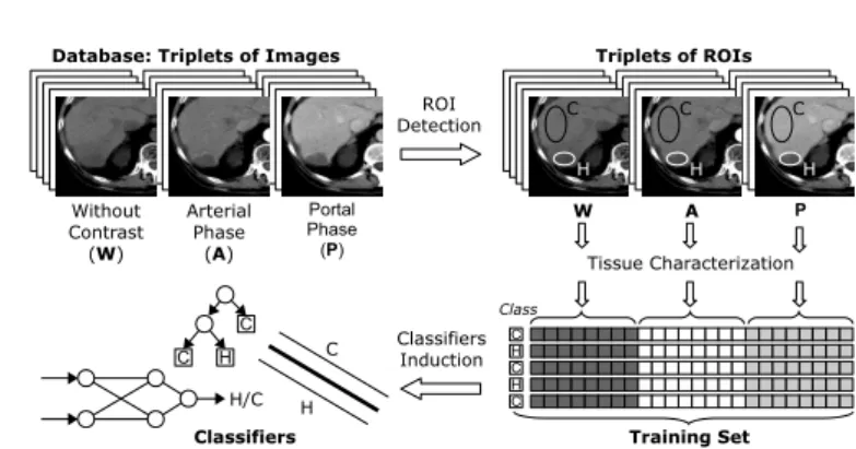
Texture-Based Classification of Hepatic Tissues

The system we develop for texture-based classification of multiphasic liver CT scans also works according to previously described two-stage model. Since typical CT exams of abdominal organs often consider three acquisition moments, which are related to the contrast product propagation in hepatic vessels, we proposed to analyze triplets of images [6], [7]. The first of the three simultaneously analyzed images corresponds to acquisition without a contrast. The second and the third are taken after its injection, at arterial and portal phases of contrast propagation. The main steps of system training are shown in Fig. 1. First, a database of image triplets (preprocessed, if needed) is created. Then a Region of Interest (ROI) is drawn at the same position on each of the three corresponding images. Each ROI is characterized by the same vector of texture parameters. Three parameter vectors are thus created, each of them characterizes a texture at different acquisition moment. In the next step, parameters from those three vectors are concatenated, in order to make one ”complex” parameter vector, describing a triplet of textures. The label representing a pathology is associated with each complex vector. At this moment, a set of labeled complex vectors could be subjected to a feature selection. Finally, it is used for the construction of the classifiers. Then the second stage of the system work can take place.

In order to recognize a new observation (see Fig. 2), a triplet of images is necessary. The three simultaneously analyzed images (in no contrast, arterial and portal phase) are subjected to the same preprocessing as it was in the training stage. Then three ROIs are drawn – one ROI on each of the three images. The triplet of ROIs is characterized in the same way as in the training stage. Finally, a complex vector of concatenated parameters (corresponding simultaneously to three acquisition moments) is classified. The tissue class that is attributed to this vector, is one of the classes considered in the training stage.

During the system design, many aspects must be investigated to ensure the best possible tissue recognition. One of them is the choice of the most relevant texture parameters. Such a choice must consider the variability of image acquisi-tion settings that could result in different image properties, like those depending on slice thickness. Some ideas for adapting the system for working with images of different slice thicknesses are presented in the next part of our study.

3.2 Parameter Stability

The estimation of parameter stability could help to decide if the parameter is re-liable for proper tissue characterization. Parameters sensitive to small changes in ROI size, or small ROI displacements, should be excluded from further analyses. We adopt the approach considered in [8] in order to assess how the parameter changes over the different ROI locations or sizes. As a measure of its changeabil-ity, the classical coefficient of variation (CV, the ratio of the standard deviation to the mean) is used. Stable parameters are characterized by low CV values, and

Fig. 1. System for texture-based classification of liver tissues: Training

Fig. 2. System for texture-based classification of liver tissues: Aiding a diagnosis

the more unstable is the parameter, the greater is its CV. In our work, the CV of each texture parameter will be calculated for different slice thicknesses.

We propose to apply the following approaches: Displace and Size Changing. In the Displace approach, the initial ROI dimensions are first slightly decreased, then the reduced ROI is displaced in order to take all the possible positions inside its initial boundaries. On the basis of each new ROI location, the value of a parameter is calculated. With the Size Changing approach, the initial ROI size is successively reduced, pixel by pixel, by moving each time one of the subsequent ROI vertices. For each of thus obtained ROIs a parameter value is calculated. In both cases, a set of several parameter values, obtained for different ROI locations (Displace) or sizes (Size Changing ) serves to calculate a CV.

3.3 Effect of Slice Thickness on Classification Accuracy

In order to evaluate the effect of slice thickness on the classification accuracy, we propose to perform several experiments, each time considering a different combination of slice thicknesses for training of classifier and for its test. If the image of a particular slice thickness is included in a training set, its counterpart (of the same slice position in a patient’s body) of another slice thickness should not be included in the test set.

3.4 Effect of Slice Thickness on Parameter Values

To access the parameter dependency of the slice thickness, we propose a similar approach that we apply for the assessment of the parameter stability. For a given parameter, its dependency on slice thickness will be measured by a ”variation” between several parameter values measured by the classical coefficient of varia-tion. These values will be obtained for the same ROI position on images of the same acquisition moment, but characterized by different slice thicknesses.

In order to validate the usefulness of the slice thickness-independent param-eters, the experiments on images with different slice thicknesses (different for a training and for a testing stage) will be performed.

4

Experiments

4.1 Database Description

The images, from 29 patients, were gathered at the Department of Radiology of the Pontchaillou University Hospital in Rennes, France. They were acquired with LightSpeed16 device (GE Medical Systems). For each patient, three scan series were performed: without contrast, at arterial and at portal phase. The contrast material, of 100 ml, was injected at 4 ml/s, in an arm vein. The arterial phase acquisitions started about 20 seconds after the contrast product injection, the portal phase acquisitions started from 30 to 40 seconds later. For each of the three scan series, two ”versions”, corresponding to slice thicknesses of 5 mm and of 1.3 mm, were available. Each thick-slice image had its equivalent in thin-slice one, with the same slice position in the patient’s body. All images had the size of 512×512 pixels. They were recorded in DICOM format, with 4096 gray levels. Since only the range of 248 gray levels sufficed for describing the pixels in the considered ROIs, the images were converted to a 8-bit BMP format.

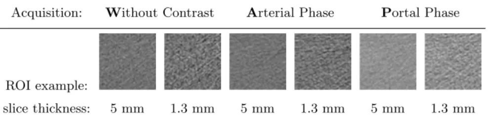
The 303 pairs of images (of a thick slice and of a corresponding thin slice) were taken into account for each of the three acquisition moments. Two classes of liver tissue were represented: cirrhotic and healthy liver (171 and 132 pairs of image triplets, respectively). A square ROI of 60×60 pixels was drawn at the same location on each of the 2·3=6 considered simultaneously images. An example of six corresponding ROIs is given in Table 1.

4.2 Texture Parameters Chosen for Evaluation

In total, 155 texture parameters, extracted with 9 methods, were tested (see Table 2). They are based on: First Order Statistics (FO), Gradients (GB), Co-Occurrence Matrices (COM) [9], Run Length Matrices (RLM) [10], Gray Level Difference Matrices (GLDM) [11], Laws Texture Energy (LTE) [12], Fractals (FB) [13], Texture Feature Numbers (TFN) [14], and Autocorrelation (AC) [15]. When applying the COM, GLDM, and RLM methods, the number of gray levels was reduced from 256, used initially, to 64. The CO Matrices and the GLD Matrices were constructed separately for 4 standard directions (0◦, 45◦, 90◦,

Table 1. Six ROIs at the same slice position

Acquisition: Without Contrast Arterial Phase Portal Phase

ROI example:

slice thickness: 5 mm 1.3 mm 5 mm 1.3 mm 5 mm 1.3 mm

135◦) and for 5 different distances between the pixel pairs, going from 1 to 5. From each of 20 thus obtained matrices, the same parameters were calculated, 11 parameters by the COM method and 5 parameters by GLDM. The RL Matrices were also constructed for 4 standard directions, each of them served to calculate 8 parameters. For the three aforementioned methods, an averaging of the same parameter corresponding to 4 different directions was done. As the result, the following parameter sets were obtained: COM55 (11·5 parameters), GLDM25 (5·5 parameters), and RLM8. The sets COM11 and GLDM5 are the result of averaging of 20 parameter values, calculated for 4 directions and for 5 distances. The normalized autocorrelation coefficients (AC) and the two TFN param-eters (among 7) were calculated separately for 5 different pixel distances, from 1 to 5. They were included, respectively, in the sets AC5, and TFN15 (with 5 other distance-independent TFN parameters). In the set TFN7, the values of 2 parameters calculated separately for the 5 distances were averaged.

The LTE method provided two parameter sets: LTE14 and LTE5. The first one, composed of 14 parameters, was obtained by the application of 24 filtering masks of size 5×5: 4 symmetric, and 10 pairs of asymmetric ones, each pair consisted of a mask and its transposition. The second set was composed of 5 parameters, corresponding to the application of 3×3 masks, 2 symmetric and 3 pairs of asymmetric ones. The sum of elements of each convolution matrix was zero. For each pair of asymmetric masks, the resulting images were added. Images obtained by the application of symmetric masks were multiplied by two. Finally, the entropies of thus obtained images served as the texture parameters. The FB method is based on the fractional Brownian motion model [16] and considers 4 pixel distances (1, 2, 3, 4). It provides a set of two parameters: FB2.

4.3 Effect of Slice Thickness on Parameter Stability

In this experiment, two approaches were applied for the CV calculation: Displace and Size Changing. The coefficient of variation was calculated on the basis of 9 parameter values. In the Displace approach, the ROI was reduced to a 58×58 square in order to take the 9 possible positions inside its initial boundaries. With the Size Changing one, the reduced ROI sizes were going from 60×60 to 52×52. The experiment was performed separately for 12 texture sets, corresponding to all combinations of: 2 slice thicknesses, 2 tissue classes, 3 acquisition moments.

Table 2. Texture parameters chosen for evaluation. In bold – parameters which later

turned out to be stable for both slice thicknesses Set Parameter Names

AC5 (d )Autocorr, where d = 1, 2, 3, 4, 5

COM55

(d )InvDiffMom, (d )SumAvg, (d )SumEntr, (d )DiffEntr, (d )Entr, (d )AngSecMom, (d )SumVar, (d )DiffVar, (d )DiffAvg,

(d )Contrast, (d )Corr, where d = 1, 2, 3, 4, 5

COM11 InvDiffMom, SumAvg, SumEntr, DiffEntr, Entr, AngSecMom,

SumVar, DiffVar, DiffAvg, Contrast, Corr FB2 FractalDim, FractalArea

FO4 Avg, Var, Skewness, Kurtosis

GB4 GradAvg, GradVar, GradSkewness, GradKurtosis

GLDM25 (d )DAvg, (d )DEntr, (d )DAngSecMom, (d )DInvDiffMom,

(d )DContrast, where d = 1, 2, 3, 4, 5

GLDM5 DAvg, DEntr, DAngSecMom, DInvDiffMom, DContrast

LTE14 E5L5, S5L5, W5L5, R5L5, S5E5, W5E5, R5E5, W5S5, R5S5, R5W5, E5E5, S5S5, W5W5, R5R5

LTE5 E3L3, S3L3, S3E3, E3E3, S3S3

RLM8 ShortEmp, LongEmp, Fraction, HighGLREmp, RLEntr,

GLNonUni, RLNonUni, LowGLREmp

TFN15 MeanConv, (d )CodeEntr, Coarse, Hom, CodeVar, ResSim,

(d )CodeSim, where d = 1, 2, 3, 4, 5

TFN7 MeanConv, CodeEntr, Coarse, Hom, CodeVar, ResSim, CodeSim

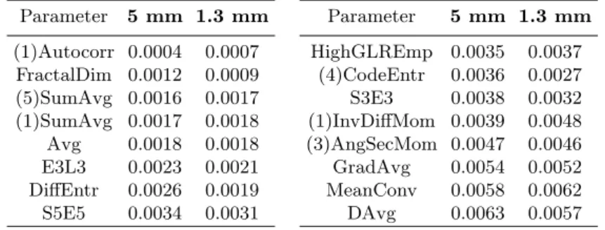
Table 3. Maximum parameter CV value (among 12 values, corresponding to: 2

ap-proaches, 2 classes and 3 acquisition moments), obtained for 2 different slice thicknesses Parameter 5 mm 1.3 mm Parameter 5 mm 1.3 mm (1)Autocorr 0.0004 0.0007 HighGLREmp 0.0035 0.0037 FractalDim 0.0012 0.0009 (4)CodeEntr 0.0036 0.0027 (5)SumAvg 0.0016 0.0017 S3E3 0.0038 0.0032 (1)SumAvg 0.0017 0.0018 (1)InvDiffMom 0.0039 0.0048 Avg 0.0018 0.0018 (3)AngSecMom 0.0047 0.0046 E3L3 0.0023 0.0021 GradAvg 0.0054 0.0052 DiffEntr 0.0026 0.0019 MeanConv 0.0058 0.0062 S5E5 0.0034 0.0031 DAvg 0.0063 0.0057

For each parameter, the CV values obtained from the same texture set were av-eraged. We observed that regardless of the approach, the three corresponding averaged CV values, obtained for three acquisition moments, did not differ

sig-nificantly. Nor did they differ between 2 tissue classes. The Displace approach almost always produced slightly higher CVs than the Size Changing approach.

Table 3 shows the averaged CV values obtained for the two different slice thicknesses. Each value is the maximum one of the 2·2·3=12 values, obtained for each combination of the approaches, classes and acquisition moments. Since the presentation of all the results occupies too much space, we present the results for 16 selected parameters. However, the CVs calculated on all 155 parameters yield the same conclusions as those obtained from the presented subset.

We can conclude, that the parameter stability, expressed by its coefficient of variation, is not considerably influenced by the slice thickness. Regardless of the extraction method, the CVs corresponding to thick and thin slices were similar. None of the thicknesses had proven to ensure better parameter stabilities.

For further experiments we decided to use the most stable parameters, for which the coefficient of variation does not exceed 0.01. The sets of parame-ters satisfying this condition were nearly identical for the two slice thicknesses. Only 4 parameters turned out relatively stable with only one of the thicknesses: CodeVar (rejected for thin slices, with CV=0.0102), Contrast, DiffVar, and Hom (rejected for thick slices, with CV equal to 0.0144, 0.0195, and 0.1721, respec-tively). In total, 93 parameters were accepted for both slice thicknesses (see bolded parameters in Table 2), and the 62 parameters were rejected.

4.4 Effect of Slice Thickness on Classification Accuracy

In this step, we considered the following combinations of slice thicknesses for training and for testing of the classifier:

– ”T/T”: training and testing performed on only thick slices (of 5 mm), – ”t/t”: training and testing performed on only thin slices (of 1.3 mm), – ”T/t”: training on only thick slices, testing on only thin slices, – ”t/T”: training on only thin slices, testing on only thick slices, – ”mix”: both thick and thin slices in a training and a testing set.

For each combination, the whole set of 303 pairs of image triplets (thick and thin version) was randomly divided into two subsets: a training set (202 pairs) and a testing set (101 pairs). For each subset, the original proportion between tissue classes was preserved. The experiment was repeated 10 times.

Table 4 presents the classification results obtained for the 5 combinations of slice thicknesses used for training and testing. Only the most efficient stable parameter sets are taken into account. Classification was performed with the Weka software [17], using Ensemble of Classifiers with adaptive boosting voting scheme [18] (AdaBoostM1 ) and a C4.5 tree [19] as the underlying algorithm.

We can observe that using the same slice thickness, both for training and for testing the classifier, results in a quite high classification accuracy. The best results are more frequent for thick slice thicknesses (”T/T” possibility). In this case, the maximal classification accuracy (86.73%) is obtained for the parameter sets COM55and RLM8. Just below the best results are those obtained when only

Table 4. Classification accuracy obtained by Ensemble of Classifiers for 5 combinations

of slice thicknesses, used for training and testing. Each line corresponds to a different set of texture parameters. Only stable parameters are considered

Set T/T t/t T/t t/T mix COM55 86.73±2.48 84.75±2.73 63.07±2.24 56.64±5.52 78.72±4.81 COM11 84.16±3.33 82.97±3.29 64.16±2.08 53.77±5.57 77.13±4.26 GLDM25 67.03±2.47 69.81±6.40 56.84±1.76 48.02±2.61 57.93±1.94 GLDM4 63.47±3.51 61.09±4.55 56.94±0.70 49.21±6.32 56.84±0.96 LTE14 78.02±3.45 78.62±2.65 58.42±2.95 44.75±8.87 69.81±3.62 LTE5 74.46±3.67 74.46±4.89 59.71±7.61 49.50±4.48 63.27±5.25 RLM8 86.73±4.43 85.15±1.81 63.96±3.65 58.82±6.65 78.62±3.65

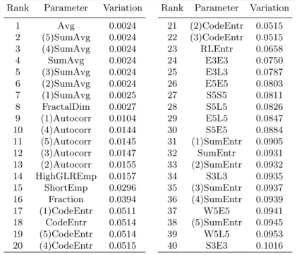
Table 5. Ranking of parameters by their dependency on the slice thickness

Rank Parameter Variation Rank Parameter Variation 1 Avg 0.0024 21 (2)CodeEntr 0.0515 2 (5)SumAvg 0.0024 22 (3)CodeEntr 0.0515 3 (4)SumAvg 0.0024 23 RLEntr 0.0658 4 SumAvg 0.0024 24 E3E3 0.0750 5 (3)SumAvg 0.0024 25 E3L3 0.0787 6 (2)SumAvg 0.0024 26 E5E5 0.0803 7 (1)SumAvg 0.0025 27 S5S5 0.0811 8 FractalDim 0.0027 28 S5L5 0.0826 9 (1)Autocorr 0.0104 29 E5L5 0.0847 10 (4)Autocorr 0.0144 30 S5E5 0.0884 11 (5)Autocorr 0.0145 31 (1)SumEntr 0.0905 12 (3)Autocorr 0.0147 32 SumEntr 0.0931 13 (2)Autocorr 0.0155 33 (2)SumEntr 0.0932 14 HighGLREmp 0.0157 34 S3L3 0.0935 15 ShortEmp 0.0296 35 (3)SumEntr 0.0937 16 Fraction 0.0394 36 (4)SumEntr 0.0939 17 (1)CodeEntr 0.0511 37 W5E5 0.0941 18 CodeEntr 0.0514 38 (5)SumEntr 0.0945 19 (5)CodeEntr 0.0514 39 W5L5 0.0953 20 (4)CodeEntr 0.0515 40 S3E3 0.1016

thin slices are considered (”t/t”): 85.15% with the RLM8 set. Slightly inferior results are observed when both slice thicknesses are considered for training and for testing (”mix”). The best of them is 78.72%, with the set COM55.

Unsatisfactory results are obtained when the slice thicknesses used for train-ing and testtrain-ing are different. Most of them do not exceed 60%. The best results for ”T/t” and ”t/T” combinations are: 64.16% and 58.82%, respectively.

We can conclude that, one should be careful using the system to aid the diag-nosis, basing on images of a slice thickness different from those used for training.

However, we suppose that, in this case, the use of the texture parameters inde-pendent of the slice thickness could improve the system performance. The search for such parameters will be the subject of our next experiment.

4.5 Effect of Slice Thickness on Parameter Values

In this experiment, we considered only those parameters that have been found to be stable for both slice thicknesses: 5 mm and 1.3 mm (see bolded parameters in Table 2). The parameter dependency from the slice thickness was expressed by the coefficient of variation of its two values, obtained from two corresponding ROIs (drawn on the images of a 5 mm and of a 1.3 mm slice thickness).

In total, 303 pairs of images were considered for each of 3 acquisition mo-ments. For each parameter, the 3·303 values of the coefficient of variation were averaged. The ranking of parameters, according to the average coefficient of variation, was performed. Parameters with the lowest average coefficient are considered as least dependent on slice thickness. Table 5 presents the ranking of the first 40 parameters which are least dependent on the slice thickness.

Since we do not know how many parameters are acceptable and sufficient for the best possible tissue recognition, when different slice thicknesses are consid-ered, we will test several sets of the first parameters from the ranking.

4.6 Classification of Textures Characterized by Parameters the Least Dependent on Slice Thickness

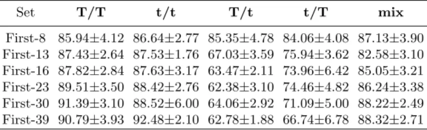
In our final experiment, 7 parameter sets were tested: First-8, First-13, First-16, First-23, First-30, and First-39. They were composed, respectively, of the first 8, 13, 16, 23, 30, and 39 parameters from the ranking presented in Table 5. Table 6 presents the classification accuracy obtained for those 7 sets by Ensemble of Classifiers (with the same settings as in the previous classification experiment). We can conclude that the classification accuracy, obtained for the 5 consid-ered combinations of slice thicknesses are similar only when the First-8 parameter set is used. This set provides the classification accuracy ranging from 84.06%,

Table 6. Classification accuracy obtained by Ensemble of Classifiers for 5 combinations

of slice thicknesses, used for training and testing. Each line corresponds to a different set of stable texture parameters, the least dependent of the slice thickness

Set T/T t/t T/t t/T mix First-8 85.94±4.12 86.64±2.77 85.35±4.78 84.06±4.08 87.13±3.90 First-13 87.43±2.64 87.53±1.76 67.03±3.59 75.94±3.62 82.58±3.10 First-16 87.82±2.84 87.63±3.17 63.47±2.11 73.96±6.42 85.05±3.21 First-23 89.51±3.50 88.42±2.76 62.38±3.10 74.46±4.82 86.24±3.38 First-30 91.39±3.10 88.52±6.00 64.06±2.92 71.09±5.00 88.22±2.49 First-39 90.79±3.93 92.48±2.10 62.78±1.88 66.74±6.78 88.32±2.71

for the ”t/T” combination, to 87.13%, for the ”mix” one. We can also notice that the application of the First-8 set guaranties the best classification results for the combinations, for which the slice thickness used for testing is different from that used for training (85.35% for ”T/t” and 84.06% for ”t/T”). For the first of these combinations, the best result is now 21.39% better than the best one obtained in the previous classification experiment, which did not consider the slice thickness-independent parameters (see Tab. 4). For the second one – the best classification accuracy augmented of 25.24%. Nevertheless, this accu-racy still remain of about 6%-8% worse than the best results obtained now for the one-thickness cases (”T/T”, ”t/t”).

In general, for the combinations ”T/t” and ”t/T”, the more numerous is the set of parameters, the worse is the classification accuracy. Contrarily, for the one-thickness cases, the classification is generally better for more numerous sets. With the ”mix” combination, the application of the First-8 set leads to ob-taining quite good classification accuracy, but not the best. In this case, increas-ing the number of parameters first results in lowerincreas-ing the classification accuracy (82.58% for the First-13 parameter set), then leads to its successive increase. Finally, the best classification result, for ”mix” case (88.32%) is obtained by the most numerous parameter set, First-39, and is 9.60% better than the best accuracy observed, for ”mix” case, in the previous classification experiment.

5

Conclusions and Future Work

The experiments allowed us to: (i ) analyze the influence of the slice thickness on parameter stability, (ii ) assess the parameter dependency on slice thickness, (iii ) find parameters which are the least dependent on slice thickness, (iv ) evaluate the classification accuracy obtained by parameters which are less and more de-pendent on slice thickness, when different slice thicknesses were simultaneously considered. Several conclusions can be formulated to sum up our study.

First, the parameter stability does not considerably depend on slice thickness. The sets of parameters recognized as stable were nearly identical for the two slice thicknesses. Second, one should be particularly careful when applying a CAD system, when recognized images are of the slice thickness different from the one used for the system training. With quite popular parameters, obtained by the COM or RLM methods, a satisfactory tissue recognition is not possible. In this case, it would be safer to use the slice thickness-independent parameters.

In the future, we plane to perform the experiments with more slice thick-nesses. Due to the fact that acquiring the series of images of many different slice thicknesses is practically impossible within a single patient study, we plane to use a phantom. It will enable to assess not only the effect of the slice thickness in the texture-based classification, but also the effect of several other parameters, like image resolution, or the time elapsed from the contrast product injection.

Acknowledgments We thank Dr D. Olivie for his precious help. This work was

References

1. Haralick, R.M.: Statistical and structural approaches to texture. Proc. of the IEEE 67(5), 786–804 (1979)

2. Guggenbuhl, P., Chappard, D., Garreau, M., Bansard, J.Y., Chales, G., Rolland, Y.: Reproducibility of CT-based bone texture parameters of cancellous calf bone samples: Influence of slice thickness. Eur. J. Radiol. 67(3), 514–520 (2008) 3. Mayerhoefer, M.E., Szomolanyi, P., Jirak, D., Materka, A., Trattnig, S.: Effects of

MRI acquisition parameter variations and protocol heterogeneity on the results of texture analysis and pattern discrimination: an application-oriented study. Med. Phys. 36(4), 1236–43 (2009)

4. Miles, K.A., Ganeshan, B., Griffiths, M.R., Young, R.C., Chatwin, C.R.: Colorectal cancer: texture analysis of portal phase hepatic CT images as a potential marker of survival. Radiology 250(2), 444–452 (2009)

5. Savio, S.J., Harrison, L.C., Luukkaala, T., Heinonen, T., Dastidar, P., Soimakallio, S., Eskola, H.J.: Effect of slice thickness on brain magnetic resonance image texture analysis. Biomed Eng Online 9:60 (2010)

6. Duda, D., Kretowski, M., Bezy-Wendling, J.: Texture-based classification of hepatic primary tumors in multiphase CT. In: Barillot C., Haynor D.R., Hell P. (eds.) MIC-CAI 2004, Part II. LNCS, vol. 3217, pp. 1050–1051. Springer, Heidelberg (2004) 7. Duda, D., Kretowski, M., Bezy-Wendling, J.: Texture characterization for

Hep-atic Tumor Recognition in Multiphase CT. Biocybern. Biomed. Eng. 26(4), 15–24 (2006)

8. Lefebvre, F., Meunier, M., Thibault, F., Laugier, P., Berger, G.: Computerized ultrasound B-scan characterization of breast nodules. Ultrasound Med. Biol. 26(9), 1421–1428 (2000)

9. Haralick, R.M., Shanmugam., K., Dinstein, I.: Textural features for image classifi-cation. IEEE Trans. Syst., Man Cybern. 3(6), 610–621 (1973)

10. Galloway, M.M.: Texture analysis using gray level run lengths. Comp. Graph. and Im. Proc. 4(2), 172–179 (1975)

11. Weszka, J.S., Dyer, C.R., Rosenfeld, A.: A comparative study of texture measures for terrain classification. IEEE Trans. Syst., Man Cybern. 6(4), 269–285 (1976) 12. Laws, K.I.: Textured image segmentation. PhD thesis, University of Southern

Cal-ifornia (1980)

13. Chen, C., Daponte, J.S., Fox, M.D.: Fractal feature analysis and classification in medical imaging. IEEE Trans. Med. Imag. 8(2), 133–142 (1989)

14. Horng, M.H., Sun, Y.N., Lin, X.Z.: Texture feature coding method for classification of liver sonography. In: Buxton B., Cipolla R. (eds.) Computer Vision – ECCV’96, Part I. LNCS, vol. 1064, pp. 209–218. Springer, Heidelberg (1996)

15. Gonzalez, R.C., Woods, R.E.: Digital Image Processing, 2nd edition, Reading, MA: Addison-Wesley (2002)

16. Chen, E.L., Chung, P.C., Chen, C.L., Tsai, H.M., Chang, C.I.: An automatic diag-nostic system for CT liver image classification. IEEE Trans. Biomed. Eng. 45(6), 783–794 (1998)

17. Hall, M., Frank, E., Holmes, G., Pfahringer, B., Reutemann, P., Witten, I.H.: The WEKA data mining software: an update. SIGKDD Explorations 11(1), 10–18 (2009)

18. Freund, Y., Shapire, R.: A decision-theoretic generalization of online learning and an application to boosting. J. Comput. Syst. Sci. 55(1), 119–139 (1997)

19. Quinlan, J.: C4.5: Programs for Machine Learning. Morgan Kaufmann, San Fran-cisco (1993)