Chaotic advection, mixing, and property exchange in three-dimensional ocean eddies and gyres

Chaotic advection, mixing, and property exchange

in three-dimensional ocean eddies and gyres

by

Genevieve Elizabeth Brett

Submitted to the Joint Program in Applied Ocean Science & Engineering in partial fulfillment of the requirements for the degree of

Doctor of Philosophy at the

MASSACHUSETTS INSTITUTE OF TECHNOLOGY and the

WOODS HOLE OCEANOGRAPHIC INSTITUTION June 2018

@2018 Genevieve Brett. All rights reserved.

The author hereby grants to MIT and WHOI permission to reproduce and to distribute publicly paper and electronic copies of this thesis document in whole or in part in any

medium now known or hereafter created.

Signature redacted

Author...

Joint ProgF m in Physical Oceanography Massachusetts Institute of Technology & Woods Hole Oceanographic Institution

May 11, 2018 Certified by... Certified by...

Signature redacted

n udte

Signature redacted~

JUN 92018

LIBRARIES

~"

Signature redacted

Larry Pratt Committee for Physical Oceanography Woods Hole Oceanographic Institution

-AMM

Chaotic advection, mixing, and property exchange

in three-dimensional ocean eddies and gyres

by

Genevieve Elizabeth Brett

Submitted to the Joint Program in Physical Oceanography Massachusetts Institute of Technology

& Woods Hole Oceanographic Institution on May 11, 2018, in partial fulfillment of the

requirements for the degree of Doctor of Philosophy

Abstract

This work investigates how a Lagrangian perspective applies to models of two oceanographic flows: an overturning submesoscale eddy and the Western Alboran Gyre. In the first case, I focus on the importance of diffusion as compared to chaotic advection for tracers in this system. Three methods are used to quantify the relative contributions: scaling arguments including a Lagrangian Batchelor scale, statistical analysis of ensembles of trajectories, and Nakamura effective diffusivity from numerical simulations of dye release. Through these complementary methods, I find that chaotic advection dominates over turbulent diffusion in the widest chaotic regions, which always occur near the center and outer rim of the cylinder and sometimes occur in interior regions for Ekman numbers near 0.01. In thin chaotic regions, diffusion is at least as important as chaotic advection. From this analysis, it is clear that identified Lagrangian coherent structures will be barriers to transport for long times if they are much larger than the Batchelor scale. The second case is a model of the Western Alboran Gyre with realistic forcing and bathymetry. I examine its transport properties from both an Eulerian and Lagrangian perspective. I find that advection is most often the dominant term in Eulerian budgets for volume, salt, and heat in the gyre, with diffusion and surface fluxes playing a smaller role. In the vorticity budget, advection is as large as the effects of wind and viscous diffusion, but not dominant. For the Lagrangian analysis, I construct a moving gyre boundary from segments of the stable and unstable manifolds emanating from two persistent hyperbolic trajectories on the coast at the eastern and western extent of the gyre. These manifolds are computed on several isopycnals and stacked vertically to construct a three-dimensional Lagrangian gyre boundary. The regions these manifolds cover is the stirring region, where there is a path for water to reach the gyre. On timescales of days to weeks, water from the Atlantic Jet and the northern coast can enter the outer parts of the gyre, but there is a core region in the interior that is separate. Using a gate, I calculate the continuous advective transport across the Lagrangian boundary in three dimensions for the first time. A Lagrangian volume budget is calculated, and challenges in its closure are described. Lagrangian and Eulerian advective transports are found to be of similar magnitudes.

Thesis Supervisor: Larry Pratt Title: Senior Scientist

Woods Hole Oceanographic Institution

Thesis Supervisor: Irina Rypina Title: Associate Scientist

Woods Hole Oceanographic Institution

Biography

Genevieve Brett, called Jay by her friends and colleagues, was raised in Connecticut. She attended Hopkins School in New Haven before studying for her B.A. in Mathematics and Physics at Skidmore College in Saratoga Springs, NY. Her first major research was done with Jim Gunton and his group at Lehigh University in the summer of 2011. She was then introduced to physical oceanography by Greg Gerbi, who joined the Skidmore physics faculty in 2011. Encouraged by Gerbi, she was a Winter Fellow at WHOI in 2012, working with Young-Oh Kwon, Magdalena Andres, and then-student Derya Akkaynak. During that fellowship, she became interested in Larry Pratt's work, which led to her joining the MIT-WHOI Joint Program later that year. After graduation, Jay will begin a postdoctoral position with Kelvin Richards of the University of Hawai'i Manoa.

Acknowledgments

Funding for this work was provided by Woods Hole Oceanographic Institution and the Office of Naval Research. The ONR support was through the MURI on Dynamical Systems Theory and Lagrangian Data Assimilation in 4D and the CALYPSO project.

I would like to thank the scientists, admins, and peers who made the Joint Program a welcoming place for me. Everyone who has asked me about my work and listened to me talk through an issue with it has contributed- thank you. Of course, I would not have gotten to this point without my advisors, who were with me at every turn, or my committee, who shared their insights. Thanks to Greg Gerbi, Magdalena Andres, and Young-Oh Kwon for my introduction to oceanography and my excellent experience as a Winter Fellow at WHOI. I also thank Mike Neubert and the math ecology group for reminding me that math is fun. My family, both biological and chosen, and especially my partner, has supported me throughout my studies. I will be forever thankful to you all, and I hope I am supporting you well in turn.

Contents

1 Introduction 25

2 Competition between Chaotic Advection and Diffusion:

Stirring and Mixing in a 3D Eddy Model 35

2.1 Introduction ... ... 36

2.2 K inem atic M odel . . . .. . . . . 38

2.2.1 Steady Symmetry-Breaking Perturbation . . . . 40

2.2.2 Comparison to Dynamic Model . . . . 42

2.3 Observing Chaotic Advection: Can it overcom e diffusion? . . . . 45

2.3.1 Scaling Derivations . . . . 47

2.3.2 Scaling R esults . . . . 53

2.3.3 Spreading of Trajectory Ensembles . . . . 55

2.3.4 Tracer Release Simulations . . . . 62

2.4 D iscussion . . . . 72

2.5 C onclusion . . . . 74

2.6 R eferences . . . . 77

3 The Western Alboran Gyre: an Eulerian Analysis of its Properties and their Budgets 81 3.1 Introduction and Background . . . . 83

3.2 M odel D escription . . . . 85

3.2.2 Model Validation ... 87

3.2.3 Model Output Description . . . . 88

3.3 R esults . . . . 96

3.3.1 Salt and Heat . . . 102

3.3.2 Dynamics of the WAG: Vorticity . . . 113

3.4 Discussion and Conclusions . . . 120

3.5 R eferences . . . 122

4 Chaotic Advection in the Alboran Sea, I: Lagrangian Geometrical Analysis of the Western Alboran Gyre 125 4.1 Introduction and Background . . . 127

4.2 M ethods . . . 129

4.2.1 M odel . . . 129

4.2.2 Velocity Field Analysis . . . 130

4.3 R esults . . . 134

4.3.1 WAG core and stirring regions . . . 134

4.3.2 Advective Transport by Lobes . . . 135

4.4 Discussion and Conclusions . . . 139

4.5 R eferences . . . 143

5 Chaotic Advection in the Alboran Sea, II: Lagrangian Analysis of Property Budgets of the Western Alboran Gyre 145 5.1 Introduction . . . 147

5.2 M ethods . . . 147

5.3 R esults . . . 151

5.3.1 Gate Transport . . . 151

5.3.2 Budgets using the gate method . . . 152

5.4 D iscussion . . . 166

5.5 R eferences . . . 168

A Rotating Cylinder Appendix A.1 Bifurcation Analysis ... A.2 Gaussian Tracer in Linear Strain A.3 Nakamura Effective Diffusivity

A.3.1 Derivation . . . . A.3.2 Long-time Limit . . . . .

B Eulerian Analysis Appendix

B.1 MITgcm Output Comparison to Climatology B.1.1 5m depth . . . . B.1.2 100m depth . . . .

B.1.3 400m depth . . . .

B.1.4 1000m depth . . . . B.2 MITgcm Eulerian Budget Methods . . . . B.2.1 Overview . . . . B.2.2 Diagnostics . . . . B.2.3 Budget Terms . . . . B.3 Western Alboran Gyre Budget Examples . B.3.1 Overview . . . . B.3.2 Full WAG salt budget . . . . B.3.3 Momentum Budgets . . . .

C Biological-Physical Interactions in the Alboran Sea C.1 Phytoplankton in the Alboran Sea: Physical Interactions

C.1.1 Introduction and Background . . . . C .1.2 Physics . . . . C .1.3 Biology . . . . C.1.4 Proposed Work . . . . C.1.5 Goal and Questions . . . . C .1.6 Approach . . . . and Functional 177 177 180 183 183 187 189 189 189 198 206 214 214 214 214 225 231 231 231 233 239 239 240 240 241 243 243 244 Types

C.2 Phytoplankton in the Alboran Sea: Persistent Productivity? . . . . C.2.1 Motivation . . . . C.2.2 Background . . . . C.2.3 Relevant Papers . . . . C.2.4 Proposed Work . . . . C.3 References . . . . Bibliography

Sources and Advection Explain . . . . . . . . . . . . . . . . . . . . . . . . Can Nutrients 246 247 247 249 251 255 259

List of Figures

1-1 Sketch of fixed points possible in two-dimensional incompressible fluid flow. Green curves are sample trajectories; black arrows are sample velocities. Left, elliptic point marked by the blue star. Right, hyperbolic point is located at the intersection of its stable manifold (blue) and unstable manifold (red). . . . . 27

I

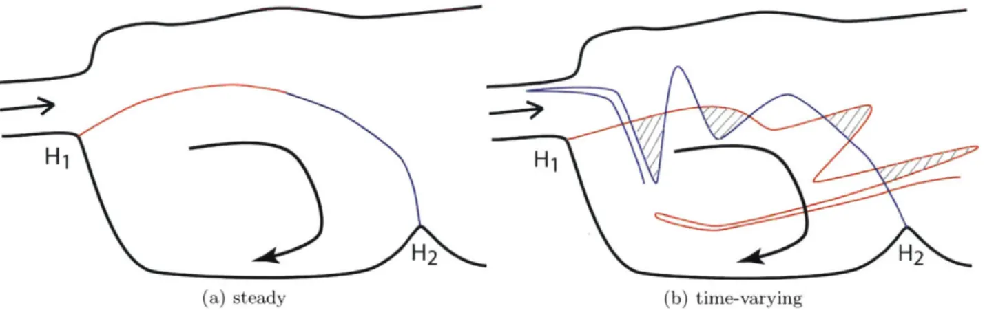
(unsta-ble) and blue (sta(unsta-ble) curves. HI and H2 are hyperbolic fixed points or trajectories. Left, steady flow, with water trapped in the recirculation for all time. The manifolds of the two hyperbolic stagnation points are a single heteroclinic streamline. Right, a periodic velocity perturbation is added to the flow. Shaded lobes map to each other in time and transport water out of the recirculation. Unshaded lobes transport water into the recirculation. . . . . 29

I

2-1 Background overturning streamfunction for a = 1 and horizontal perturbation stream-function for y = 2, xo = -0.5. Left to right: overturning E = 0.125, E = 0.02,

E = 0.0005, horizontal perturbation. Note the vertical structure in the overturning streamfunction becoming similar to Taylor columns as E gets smaller. Note that the center of rotation in the perturbation streamfunction is not at the origin. . . . . 41

2-2 Structures in the kinematic model and dynamical simulation for Ekman numbers of 0.25 and 0.125, continued on next page. . . . . 45

2-2 Structures in the kinematic model and dynamical simulation for Ekman numbers of (a) 0.25 and 0.125, (b) 0.02 and 0.0005. Tops: Poincar6 maps from Pratt et al. 2013, using the dynamic simulation. Bottoms: in black, Poincar6 maps from the current kinematic model with E = 0.01 and xO either -0.5 (left) or -0.9 (right); in color, maximum FTLEs calculated for the kinematic model with integration time 400. For

E = 0.125, red oval approximately separates the resonant and regular layers (inside) from the chaotic sea region (outside), with the blue line segment showing the width of the chaotic sea. The blue diamond shows the width of an island, which is also the width of the resonant layer. . . . . 46

2-3 An initial sphere in a linear strain field evolving into an ellipsoid during a time of 1. Ellipsoid axes marked by bars, with figure axes ticks showing their initial values of 1 and their individual endpoint values. Color shows z values at t = 0, demonstrating the contraction in the z direction. Velocity field u = 1.5 + x, v = 0.5y, w = -1.5z. . 50

2-4 Layer widths in blue, Lagrangian Batchelor scale 6 in the same region in yellow. Left half, chaotic resonant region between islands; right half, the chaotic sea region. The diffusivities at the Batchelor scale in m2

/s

2-5 Diffusive crossing times for islands compared to chaotic advection timescale for ad-jacent chaotic resonant layer. Uses Okubo's estimate of diffusivity for the island

w idth . . . . 56

2-6 Grey lines are individual trajectories in 0 starting from a sphere of radius 0.002 at

(r, z) = (0.1, 0.5) with E = 0.125. Solid black curves are the mean; black dash-dot lines are +1 standard deviations from the mean. . . . . 58

2-7 Range in 4 for ensembles of trajectories started from a sphere of radius 0.002. Steady perturbation (c E {0.01, 0.081), stochastic perturbations (n E {10-5, 10-6 10-7}), or both (K = 10-7, E = 0.01), are added to the background flow. Left: Initial sphere in the chaotic sea region, away from fixed points, at (r, z) = (0.1, 0.5). Right: Initial sphere centered on (r, z) = (0.4, 0.5), a resonant region. . . . . 61

2-8 Top, tracer variance,

x

;

neff

E

bottom, xO = -0.02, k = 10-4. The xo = 0, k = 10-6 case is not shown, but is qualitatively similar to the xO = 0 k = 10-4 case. Top: Dye, t = 39. Row 2: Keff, t = 39. Row 3: Dye, t = 299. Bottom: neff, t = 299. . . . . 69 2-10 E = 0.125 for three steady perturbation levels: left, xo = 0; middle, xo = -0.02;

right, xo = -0.16. Top: Dye, t = 39. Row 2: /'eff, t = 39. Row 3: Dye, t = 299. Bottom : ef _{f, t = 299. . . . . 70} 2-11 E = 0.02 Poincar6 sections in the (a)x - z and (b)y - z planes in black. Polygons

show the island (blue) and resonant (red) regions used for analysis (c) and (d), mean Keff over time in these regions under both applied background diffusivities. The no-chaos match case is the same area as the island in the unperturbed flow. . . . . . 71

3-1 (a) Domain of the simulation. Color is bathymetric depth, black curves are coast. Black lines on land indicate approximate borders between Portugal and Spain (north-ern) and Morocco and Algeria (south(north-ern). (b) Model grid, with every 10th gridline in blue over the area of each cell in reds (m2

), and the coast indicated in black. (c) Depth grid spacing in meters, top 40 interfaces, interfaces 1, 10, 20, 30, and 40 labeled. 86 3-2 Monthly mean SSH (saturated colors at 0.2m red and -0.2m blue), comparison

between MITgcm output and AVISO data. November 2007 through June 2008. . . . 89 3-3 Monthly mean SSH (saturated colors at 0.2m red and -0.2m blue), comparison

between MITgcm output and AVISO data. July through December 2008 . . . . 90 3-4 Daily SSH correlation (y - axis position and color) between output and observations

3-5 (Top) Mean SSH (m) over the 148-day well-correlated period, comparison between MITgcm output (left) and AVISO data (right). (Bottom) Standard deviation of daily SSH (M2) over the same period. . . . . 92 3-6 (a) Outflow (Sv) from all depths along a meridional section going through

Sam-martino et al.'s mooring location compared to SamSam-martino et al.'s subinertial outflow measurement. (b) Interface depth (meters below surface). Measured is Sammartino et al.'s zero-crossing from mooring data. Model interface is defined by the bottom of the deepest cell where the mean across-section flow is toward the Alboran. In both, the black vertical line indicates the end of the 148-day period analyzed further. . . . 93 3-7 Mean surface salinity of the 148-day analysis period in greens with the chosen WAG

boundary in red. Blue dashed lines indicate the location of sections shown in the next figures. . . . . 94 3-8 Two north-south sections, facing west, of the 148-day mean zonal velocity field with

mean potential density contours overlaid. Left, in the Strait of Gibraltar. Right, in the W estern Alboran Gyre. . . . . 94 3-9 Two north-south sections, facing west, of the 148-day mean potential density field,

blues, with mean salinity contours overlaid. Left, in the Strait of Gibraltar. Right, through the Western Alboran Gyre . . . . . 95 3-10 Two north-south sections, facing west, of the 148-day mean salinity field, reds, with

mean potential temperature contours overlaid. Left, in the Strait of Gibraltar. Right, through the Western Alboran Gyre . . . . . 95 3-11 Total Euler WAG volume budget, m3/s. These are the net volume transports through

the sides (dark blue), bottom (dark green), and top (red), and the volume transport form of the change in storage due to changing SSH (light blue). . . . . 97 3-12 Magnitudes of the Euler WAG volume budget, m3/s. These are the gross volume

transports, the sum of the absolute value of the volume transport through each cell edge at the boundaries of the Eulerian WAG. . . . 100 3-13 Mean vertically-integrated advective volume transports for the Euler WAG. Colors

show transport through the bottom, arrows show transport through the sides. Top left arrows show scale, 5. 105m3/s. White patches indicate seamounts. . . . 100

3-14 Euler WAG net vertical volume transport is primarily the Oo = 27.5 isopycnal moving across the fixed bottom boundary, which is its mean depth. The vertical volume transport and the derivative of the volume above the isopycnal in the WAG are shown. These correlate with r = 0.7447 and p < 0.0001 . . . 101 3-15 Top, total Euler WAG heat budget, J/s. Bottom, mean vertically-integrated

advec-tive potential temperature transports for the Euler WAG. Colors show flux through the bottom, arrows show flux through the sides. Top left arrows show scale, 5 -1010 Cm3/s. Seamounts do not appear as empty space as they did for the mean

vol-ume transports because the transport across the bottom-most wet cell is used rather than the o- surface. . . . 104 3-16 Top, Euler WAG heat budget, J/s, with the transports of heat by the volume

ports of the mean gyre temperature, 16.99'C, removed. Bottom, time-mean trans-ports of heat, J/s, with the transtrans-ports of heat by the volume transtrans-ports of the mean gyre temperature removed. Terms are, left to right, advection through the sides, advection through the bottom, vertical diffusion, surface forcing, -dH/dt, and the sum of the term s. . . . 105 3-17 Top, Euler WAG heat budget, J/s, advection combined, with the transports of heat

by the volume transports of the mean gyre temperature, 16.990C, removed. Bottom, same budget, with advection and -dH/dt combined to show smaller terms. . . . 106 3-18 Potential temperature at 25m on simulation days 220, 240, 245, 250, 255, and 260.

Day 220 is typical of the case where the AJ is attached to the African coast. The remaining days show how the AJ carries Atlantic water that forms a recirculation of nearly W A G size. . . . 107 3-19 Potential temperature at 75m on simulation days 220, 240, 245, 250, 255, and 260.

Day 220 is typical of the case where the AJ is attached to the African coast. The remaining days show how the AJ carries Atlantic water that forms a recirculation of nearly W A G size. . . . 108 3-20 Euler salinity minimum region volume-integrated salt budget, g/s. Top, all terms;

bottom, advection terms combined. In the legends, 'h' indicates horizontal, 'z' indi-cates vertical, and 'adv' is for advection. . . . 110

3-21 Euler salinity minimum region volume-integrated salt budget, g/s, time means. Left to right, terms are the total of the advection terms, the vertical diffusion, the negative changes in salt content, and the sum of these terms. . . . 111 3-22 Salinity at 50m on simulation days 220, 240, 245, 250, 255, and 260. Day 220 is

typical of the case where the AJ is attached to the African coast. The remaining days show how the AJ carries Atlantic water that forms a recirculation of nearly W A G size. . . . 112

3-23 Mean surface relative vorticity normalized by planetary vorticity,

f,

3-24 Vorticity budget for the Eulerian WAG, volume-integrated terms, m 3/S2. Pressure

and model time-stepping terms not shown, on the order of 10- 5m 3/S 2. Coriolis term not shown, less than

1m

3-25 Time means of the volume-integrated vorticity budget terms, m3/s 2, 148-day period

in blue bars, red stars for each month's means. . . . 116 3-26 Euler WAG area-integrated vorticity budget in horizontal layers, mean of all terms

vs. layer center depth, m2_/S 2_{. Top, full 148-day mean; left, first 74-day mean; right,}

last 74-day mean. Dissipation is the combination of drag and horizontal diffusion. . . 117 3-27 Euler WAG area-integrated vorticity budget in horizontal layers, mean of all terms vs.

layer center depth, m2/S2 . Left, full 148-day mean; right, 148-day mean magnitudes.

The decay in the diffusion term has a scale of about 37m. . . . 118 3-28 Mean velocity at 170m (a) and 250m (b) over the 5 months analyzed. Note the

westward current along the southern coast that connects to the outflow through the Strait of G ibraltar. . . . 118

4-1 Surface stable manifold integrated over 14 days from two different initial positions. Note that in the interior of the Alboran Sea, these two calculations match. . . . 132

4-2 Definition Figure : Unstable (red) and stable (blue) manifolds . Hyperbolic points HI, H2. Left, steady. Water is trapped in the gyre for all time. Right, periodic. Shaded lobes map to each other in time and transport water out of WAG. Unshaded lobes transport water into WAG. . . . 132

4-3 Manifolds on the surface and 5 isopycnals using the 148-day mean flow. Integration time 14 days, resolution 2km. Red, unstable manifold; blue, stable manifold; thin black contours, isopycnal mean depth; thick black, coast. . . . 133 4-4 Probability of a manifold crossing each location on a given day, color. Daily horizontal

velocities 8-day integration, 2km resolution. For (b)-(e), black contours are mean isopycnal depth and velocities are horizontal at the daily depth of the isopycnal. Contrasting color is the zero probability curve of the probability field. . . . 136 4-5 _{Probability of a manifold crossing each location on a given day. Surface velocity,}

8-day integration, 2km resolution. (a)Unstable manifold. (b)Stable manifold. . . . . 137 4-6 The center region of the WAG. Zero contour of the manifold probability field from the

surface and 4 isopycnals (og = 26.75 skipped for readability). Left, 8 day manifolds. Right, 14 day m anifolds. . . . 137

4-7 Lagrangian WAG edge (green dashed curve) using gate to connect the unstable (red) and stable (blue) manifolds. A lobe is visible near (-3, 36). Note the complicated folding of the m anifolds. . . . 139

4-8 Evolution of one lobe in 2D and 3D. (a) Points inside the lobe are shown on simulation days 13, 15, 17, and 19 at the surface, with the manifolds from day 15 also shown. (b) Points show the edges of the lobe on days 15, 17, and 19 at the surface and on isopycnals oo = 26.5, ao = 27 which are sections of the stable and unstable manifolds on those surfaces. Bottom topography is shown with purple deeper regions; green curves on the topography are the projection of the

o

or the top grid cell (5m). Lobes were used to estimate fluxes into the WAG, assuming a 2 day tim escale. . . . 141

5-1 Definition Figure : Unstable (red) and stable (blue) manifolds . Hyperbolic points H1, H2. Left, steady. Water is trapped in the gyre for all time. Right, periodic. Shaded lobes map to each other in time and transport water out of WAG. Unshaded lobes transport water into WAG. Orange gate connecting the manifolds allows a well-defined gyre boundary. . . . 148

5-2 WAG Lagrangian boundary on the surface in blue. Red dashed curves are the pre-vious day's offshore boundary advected forward one day. Axes are longitude and latitude. ... ... 149

5-3 WAG Lagrangian gate for simulation day 19. The gate locations at the surface and on

5

5-4 Advective transports through the gate at each layer and total for volume (a, top), salt (b, bottom); more on next page. . . . 153

5-4 Advective transports through the gate at each layer and total for volume (previous page), salt (previous page), heat (c, top), and vorticity (d, bottom). . . . 154

5-5 Advective transport through the gate compared with that done by the volume trans-port at a representative salinity, temperature, or vorticity. . . . 155

5-6 WAG edge at co = 26.5 (blue) and og = 27.5 (green) on day 38 of the simulation for illustration. Advection through the gate is represented by red arrows. Volume transport implied by the diffusive movement of o = 27.5 will occur over its whole area. That from diffusive movement of the

ao

5-7 WAG volume budget for the region defined by the uo = 27 manifolds and ending at

o0 = 27.5. Red stars indicate days with known problems of ill-defined boundaries,

fast time dependence, or large errors in dV/dt from manifold surgery. Transports in

5-8 Lagrangian budget error examples. Left top, uo manifolds for simulation day 62 with 14 day integration do not reach the gate location of 4.4'W. Right, surface manifolsa and boundary on simulation day 20. Note the complicated and self-intersecting edge in the southwest. Bottom, co manifolds for simulation days 61 and 62, over which the gate moves farther than its width. . . . 160 5-9 Example of terms in an hourly Lagrangian volume budget over simulation days 20 and

21. Left, volume transport comparison between daily and hourly. Right, comparison of the hourly gate transport and changes in Lagrangian volume. . . . 161 5-10 WAG volume budget for the full analyzed section, surface to UO = 27.5. Red stars

indicate days with known problems of ill-defined boundaries, fast time dependence, or large errors in dV/dt from manifold surgery. Transports in m3/s for the 148 days

analyzed . . . . 163 5-11 WAG volume budget for the time periods without known large errors, surface to

ao

/s.

heat, and vorticity. . . . 165 5-13 Comparison of transport through the sides of the WAG from the Lagrangian and

Eulerian analyses. Transport of volume, salt, heat, and vorticity are shown. . . . 167

A-1 Height of rz-fixed points in the vertical plane at r = 0.5a. Black indicates elliptic points, blue hyperbolic, gray the neutrally stable points at the top and bottom. New fixed point pairs separate symmetrically from z = 0.5 as E decreases. At each bifurcation, the central fixed point changes stability. . . . 179 A-2 Trajectories in the vertical plane for E = 0.00125, a = 1. There are 9 rz-fixed points

along r = 0.5, marked with red stars. Note the closed curves between the outermost hyperbolic points which surround the interior 5 rz-fixed points; these limit the effects of those points to the local area. . . . 180

B-i Potential temperature budget with daily-averaged fields for two months. Fluxes are totals for the Eulerian Western Alboran Gyre. Red dashed line is the error. . . . 230

B-2 Top, total Euler WAG salt budget, g/s. Bottom, mean vertically-integrated advective salinity fluxes for the Euler WAG. Colors show flux through the bottom, arrows show flux through the sides. Top left arrows show scale, 5. 1010[c]m3/s, where [c] is salinity

units. Seamounts do not appear as empty space as they did for the mean volume fluxes because the flux across the bottom-most wet cell is used rather than the UO surface. . . . 232

B-3 Top, total Euler WAG salt budget with volume transport of water with mean WAG salinity, 36.61, removed. Bottom, time-mean transports of salt, g/s, with the trans-ports of salt by the volume transtrans-ports of the mean gyre salinity, 36.61, removed. . . 234

B-4 Euler WAG salt budget, advection combined, g/s, with the transports of salt by the volume transports of the mean gyre salinity, 36.61, removed. . . . 235

B-5 Euler WAG salt budget, smaller terms, g/s, with the transports of salt by the volume transports of the mean gyre salinity, 36.61, removed. Negative peaks in the surface

term are rain. . . . 235

B-6 Euler WAG volume-integrated momentum budget, all terms, m4/s2. Top, zonal; bottom , m eridional. . . . 237

B-7 Euler WAG volume-integrated momentum budget, m4/s2, secondary terms (largest

terms, Coriolis and pressure gradient force, are combined into the 'ageostrophic' term). Left, zonal; right, meridional . . . 238

B-8 Euler WAG volume-integrated momentum budget in horizontal layers, mean of all terms vs. layer center depth, m4/s2. Left, zonal; right, meridional . . . 238

C-1 (a)Schematic of the Alboran. This is one of several quasi-equilibrium states commonly observed. CCG is the Central Cyclonic Gyre. (b) An example MITgcm daily mean surface velocity plotted over bathymetry. Note the WAG at about 4W. . . . 241

C-2 PHYSAT-Med applied to MODIS data (2002 to 2013): monthly climatology of dom-inant PFT. Top row: Jan, Feb, Mar. Each pixel is marked as one of: 0 unidentified, 1 nanoeukaryote, 2 prochlorococcus, 3 synechococcus, 4 diatom, 5 phaeocystis, 6 coccolithophorid. The Alboran is dominated by nanoeukaryotes and synechococcus, with diatoms in Nov-Feb. (Adapted from Navarro et al. 2014.) . . . 243 C-3 Mean SSH in the Alboran Sea for 2008 from the MITgcm (left) and AVISO (right). 244

C-4 Variability of the contribution of three size fractions of plankton to the total chl-a. Stations (A,B,C) were visited every 3 days (4 times total) during a cruise in May 1998. The location is in the northern portion of the WAG. (From Arin et al. 2002) 246 C-5 Mean primary production across the Mediterranean. Generally productivity

de-creases from West to East and from coastal areas to deeper water. (Coll et al. 2010)... ... 247 C-6 Climatology of December chl from 9 km gridded monthly SeaWiFS in color. Magenta

curves are isobaths. (Oguz et al. 2014) . . . 248 C-7 Climatological diffuse attenuation coefficient (1/m) from MODIS 9km for 490nm.

No appreciable difference is found using MODIS 4km. (MODIS data and Giovanni visualization by GES DISC, Acker and Leptoukh 2007) . . . 252 C-8 Climatological surface nitrate concentration (mmol/m3) from MEDAR. (a) Full

cli-m atology (b) W inter only. . . . 253 C-9 Typical behavior of the NP model with time. Parameters as given as initial values

in Table C.1, with initial N = 1, P = 0.01, 0.1. . . . 254 C-10 Sample points from trajectories from surface MITgcm velocities. All initial points

(black shading) are in the Strait of Gibraltar, east of the Camarinal Sill; daily releases for 45 days. Blue points are positions 6 days after release, red points are positions 10 days after release. . . . 254 C-11 Sample P field from one-month set of daily releases of trajectories throughout Alboran.255

List of Tables

3.1 Time-mean volume transports across the Euler WAG boundaries, m3/s, positive into

the gyre, rounded to three significant digits. . . . . 98

B.1 Table of diagnostic names and what they contain, plus grid measures needed for budgets and background stratifications. . . . 222 B.2 Table of diagnostic names and what they contain. This set of diagnostics can close

the salinity and temperature budgets. . . . 223 B.3 Table of diagnostic names and what they contain. This set of diagnostics can close

the horizontal momentum and vertical vorticity budgets. . . . 224

Chapter 1

Introduction

Oceanographic models and theories are traditionally Eulerian, examining the ocean from a fixed reference point. The Eulerian viewpoint is also very useful for creating maps of water properties from observations, such as is done for the World Ocean Climate Experiment and Global Ocean Ship-based Hydrographic Investigation Program repeat sections. This view is also convenient for theories of the steady circulation in a basin, such as the traditional Stommel and Munk gyres. However, when considering the evolution of the properties of a parcel of water, a Lagrangian view is more natural. A Lagrangian view is in the frame of the fluid, such that the coordinates are functions of time. Lagrangian measurements of tracers and of the tracks of drifters and floats have improved our knowledge of, for example, the North Atlantic Deep Western Boundary Current (DWBC). The paths followed by water parcels, as measured by floats and drifters, are generally more convoluted than the spatially and time-averaged Eulerian maps of ocean currents would suggest. For example, the path of the DWBC was considered fairly direct, southward along the continental slope, before tracer and float studies demonstrated that there are recirculations eastward into the interior (see Fine 1995 for a review). The possible effects of these recirculations can be demonstrated in laboratory flows (Deese et al. 2002), where stretching and folding of a tracer can cause enhanced mixing, an idea I will return to. Pathways from the boundary current to the interior are also important for the meridional overturning circulation, as these paths demonstrate that newly formed deep waters can spread to the interior of the basin fairly quickly (Bower and Hunt 2000).

The analysis of trajectories from drifters and floats represents a particular case of kinematic analysis of the ocean. Kinematic analysis of geophysically-relevant flows have been improved over

the past few decades by the introduction of methods based in dynamical systems theory. I will discuss some of the basic terminology and analyses used for dynamical systems as background. Then I will provide an overview of the types of objects identified in oceanographic applications, before introducing the questions addressed in my research. This background is not a comprehensive review, but rather intended to provide a qualitative understanding of the state of the field so that the impact of the following research is clear.

A dynamical system analysis applies to differential equations or systems thereof. In a determin-istic system where the behavior is known over infinite time, the structure of many trajectories, or paths in time, through the phase space can be identified through invariant surfaces: surfaces that trajectories are trapped on. The simplest case of an invariant surface is a fixed point: a location in the system which, when used as the initial condition, produces a trajectory'that does not change with time. In a fluid system, a fixed point is a stagnation point. The qualities of a fixed point depend on the trajectory of nearby initial conditions. Such nearby trajectories may approach the fixed point, move around it at a (nearly) fixed distance, or move farther away. If all points nearby behave in the same manner, the fixed point may be classified as stable, neutrally stable, or unstable, respectively.

In the case of a two-dimensional incompressible fluid flow, a fixed point can be classified as elliptic or hyperbolic (sketches in figure 1-1). Elliptic points are neutrally stable; a physical example is a stagnation point in the center of a steady vortex, where trajectories remain at a similar distance from the center over all time. Flows around a hyperbolic point follow hyperbolic trajectories, approaching and then accelerating away from the point. For hyperbolic points, stable and unstable manifolds are curves along which all points asymptotically approach the fixed point in forward or backward time, respectively. Other trajectories approach the region of the fixed point in the direction of the stable manifold and leave the region in the direction of the unstable manifold. With increased numbers of dimensions, the possible geometries of fixed points increase, although the stability can be defined in the same fashion.

Dynamical systems may also have features of interest that are of higher dimensions than points. These include the manifolds associated with hyperbolic fixed points, which organize the nearby trajectories' hyperbolic shape. Another example is closed trajectories, which indicate repeating oscillations of the system and may themselves be stable or unstable. Trajectories may also be

(a) elliptic (b) hyperbolic

Figure 1-1: Sketch of fixed points possible in two-dimensional incompressible fluid flow. Green curves are sample trajectories; black arrows are sample velocities. Left, elliptic point marked by the blue star. Right, hyperbolic point is located at the intersection of its stable manifold (blue) and unstable manifold (red).

confined to sub-sections of the space, such as along spheres or planes in a 3-dimensional system. It is a general rule that trajectories may not intersect, so if there is a closed curve, for example, in a two-dimensional system, then all trajectories starting inside (outside) that curve must remain inside (outside) for all time. This is true for any material curve in a fluid as well, provided there is not droplet formation. The goal of the dynamical systems-based methods developed for application to geophysical fluids is to identify material contours that are maximal in some sense compared to their surroundings and provide insight into the structure of the flow, generally using information about the flow over a finite time. I will describe two types of contours that are of interest: least-stretching closed contours and most-stretching open contours, each used to identify a different aspect of ocean features.

Least-stretching closed material contours are usually within a set of closed material contours surrounding a vortex or eddy. The minimal stretching of the material indicates that it does not undergo filamentation and can therefore be considered to bind the water inside such that it is not stirred with its surroundings over time. Eddies with such bounding contours are called coherent, and there are quite a few methods that may find these contours (see Hadjighasem et al. 2017 for a review). Separating these coherent eddies from others is a case where Lagrangian analysis has improved our understanding of ocean processes.

Eddies appear ubiquitous in altimetry as anomalous sea-surface heights (and anomalous vortic-ities) that retain this signature over time. Some persistent recirculations are locally very important for the flow; examples include the Great Whirl and the Western Alboran Gyre. Other eddies move in space, often at rates similar to Rossby waves, such as rings that separate from the Gulf Stream and Kuroshio. The extent to which these various eddies are coherent is uncertain. The transport of water by the moving eddies is important for understanding how these observed eddies may con-tribute to global meridional heat transport, for instance. A large study tracking sea-surface height anomalies by Dong et al. (2014) suggested that these eddies might contribute 20% of the global meridional heat transport. However, a study using transfer operators by Froyland and coauthors (2012) showed that anomaly eddies do not consistently transport water, instead exchanging water with their surroundings. The exchanging eddies are then somewhat wavelike anomalies, a clear signal but not a consistent transport process. A study by Abernathey and Haller (2018) used a La-grangian method to identify coherent eddies, which do carry water with them. These are generally smaller and shorter-lived than eddies tracked with Eulerian measures, contributing 1% or less to the meridional heat transport of the ocean, which is much smaller than the earlier estimate. The updated idea from this series of studies is that mesoscale eddy motions, including long-lived moving sea-surface height anomalies, are mostly stirring the water, not coherently transporting eddies with disparate properties. However, this has not yet been examined for the more persistent recirculations.

Most stretching (open) material contours identify strong stirring regions in a fluid flow. These can be the manifolds of hyperbolic trajectories, a generalization of hyperbolic fixed points and their manifolds. I use a coastally-trapped recirculation as an example, first with steady flow and then with a time-periodic perturbation (see figure 1-2 for a sketch). In the steady case, there are two stagnation points on the coast. The outer limit of the recirculation is a streamline connecting these points. These stagnation points are hyperbolic, with convergent and divergent flow nearby. For

H1, there is convergent flow along the coast towards the stagnation point and divergence in the

offshore direction, while the opposite is true for H2. With a small perturbation to a time-dependent

flow, these stagnation points no longer exist, but are each replaced by a hyperbolic trajectory in the same neighborhood. Then each trajectory has one offshore manifold, but these no longer match each other. The unstable manifold of H1 and the stable manifold of H2 cross repeatedly, trapping water

H1

H

Figure 1-2: Sketch of a coastally-trapped recirculation. Manifolds are represented by red (unstable) and blue (stable) curves. HI and H2 are hyperbolic fixed points or trajectories. Left, steady flow, with water trapped in the recirculation for all time. The manifolds of the two hyperbolic stagnation points are a single heteroclinic streamline. Right, a periodic velocity perturbation is added to the flow. Shaded lobes map to each other in time and transport water out of the recirculation. Unshaded lobes transport water into the recirculation.

exterior flow; in the figure, the shaded lobes move water out of the recirculation and the unshaded lobes move water into the recirculation. When the time-dependent perturbation is periodic, the shape of the manifolds will be periodic, with water moving from one lobe position clockwise to the next in each period, shaded lobes mapping to shaded lobes and unshaded to unshaded (see Wiggins' book for mathematical theory). In a simplified system with wind-driven barotropic (depth-independent) flow, Miller et al. (2002) were able to identify these lobes and calculate the related transport. For realistic strengths of the wind forcing, the transport of volume by lobes was larger than the Ekman pumping by the wind. For a realistic simulation of the a Gulf of Mexico eddy, Branicki and Kirwan (2010) were able to show the structure of lobes in three dimensions but did not continue to a transport calculation due to the difficulty of calculation of the lobes' volume.

It is important to realize that the periodic flow described above, with their periodic manifolds, will generally contain aperiodic trajectories. These aperiodic trajectories, including those in the lobes, undergo exponential stretching and folding, separating far from initially-nearby trajectories in time. This behavior of aperiodic trajectories whose later positions are very sensitive to initial conditions is called chaos or chaotic advection. Chaotic advection was introduced to the fluid dynamics community by Aref (1984) to describe nearly-integrable flow that is sensitive to initial conditions and causes fast stretching and folding of trajectories and water parcels. The stretching

and folding are controlled by long-lived structures, meaning that the lifetime of the structures is longer than the time it takes a trajectory to orbit them. This separation of timescales allows regions of chaotic and non-chaotic flow to be identified before the flow structure changes. Least-stretching material contours organize non-chaotic regions, while exponentially stretching manifolds organize chaotic regions.

The turnstile lobes defined by crossing manifolds directly relate to the transport between two different regions of the flow. However, they not only transport the fluid, but also stir it. The lobes become very stretched out near the hyperbolic trajectories, as the manifold of the farther hyperbolic trajectory repeatedly folds over the manifold of the nearby trajectory. This stirring is such that if there is a difference in water properties between the interior and exterior regions, the gradients will be greatly enhanced, in turn enhancing mixing. I will next discuss the relationship between stirring and mixing, which underpins much of the research to follow.

Stirring is a reversible process of shear causing the stretching and contracting of a water parcel. For instance, kneading dough is primarily stirring it, spreading new flour across the existing dough in a very thin layer and folding it into many thin layers. Mixing, by contrast, is an irreversible process where properties become homogenous. Molecular diffusion is a canonical case of mixing, where molecules of two substances, particularly liquids or gasses, become arranged in space in a statistically homogenous distribution through the random motion of molecules due to their temper-ature (kinetic energy). Turbulent diffusion is an analogous process where turbulent flow exchanges fluid parcels with different properties, such that the properties spread through an area and become more homogenous. Reynolds averaging in a system with scale separation is often used to describe a turbulent diffusivity related to the kinetic energy of small motions.

A Lagrangian view allows for clearer consideration of stirring and mixing than an Eulerian view. Tracking of water parcels through trajectories can allow direct measurement of the stretching and folding they undergo through the separation of trajectories in time. Eulerian measurements, by contrast, only allow evaluation of stretching in a location. As water parcels move, they experience different stretching rates in different locations. The ergodic theory supposes that the total space is sampled by any trajectory, and is sometimes used to avoid considering Lagrangian information. However, in the ocean, physical constraints such as potential vorticity conservation organize the flow, such that ergodicity is less reasonable.

If trajectories and their separations are measured following a water parcel, associated measure-ments of tracers over time shows the rate at which mixing occurs. Stirring can speed mixing by creating large gradients between adjacent water parcels and increasing the surface area over which exchange can occur. A good image is coffee and cream. If coffee and cream are initially added to a container so that they have only one interface and they are both at rest, mixing can only occur across that interface and will be due to molecular motion alone. Away from the interface, molecular diffusion is mixing each fluid with itself, effecting no change. If the container is stirred, intrusions of each fluid into the other will rapidly increase the surface area of the interface where molecular motion can exchange coffee and cream molecules in space, leading to a mixture indicated by chang-ing color. Coherent eddies in the flow, with their non-filamentchang-ing edges, are a particular case with slow mixing. By contrast, chaotic regions in the flow, likely contraining hyperbolic manifolds, will have high stirring rates and fast mixing.

The following chapters will examine two modeled physical systems, an eddy and a gyre. The eddy model is an extension of work by Pratt et al. (2013), which identified the chaotic and regular regions of the flow. I consider whether diffusivity will be important in this system in regards to tracers. There are two complementary issues. First, I consider whether the separation between chaotic and non-chaotic, or regular, regions will survive the addition of diffusion. This survival is important if observational ocean studies are ever to confirm the existence and behavior of Lagrangian structures at submesoscales. In order to observe a chaotic region using dye, for example, the dye would need to be advected along the structure without diffusively spreading out into other flow regions. In essence, the chaotic stretching must dominate over diffusion in the flow's behavior for long enough to take an effective observation. While this may be assumed for a mesoscale ocean feature, at smaller scales diffusion is a more significant component of the tracer evolution. The second question addresses the enhancement of mixing through stirring. Any stirring enhances mixing, but I examine how much chaotic regions increase mixing over regular regions that are stirred. This work is covered in Chapter 2.

The second system, the gyre, is coastally trapped in a geometry like figure 1-2. Either this type of structure, or a double-gyre, has been repeatedly studied in the Lagrangian method literature as a straightforward system with chaotic and regular regions. However, these are usually simplified, with the flow being time-periodic, two-dimensional, or both. I realistically model a three-dimensional

aperiodic gyre. I identify the manifolds at the surface and along isopycnals as an approximation of the three-dimensional structure of the manifold surfaces and show an example of a three-dimensional lobe. I also use this setup to quantify the exchange of water into and out of the gyre, which may be the first such analysis for such a realistic system. This exchange forms part of the budgets for volume, heat, and salt of the gyre, and I compare Lagrangian and Eulerian budgets to understand the physical dynamics of the gyre. The model description and Eulerian analysis of the physics in the mean gyre location are covered in Chapter 3. Chapters 4 and 5 present the Lagrangian analysis and discuss the differences from the Eulerian results.

Overall, the following research aims to investigate some aspects of how a Lagrangian perspective applies to oceanographically relevant flows. Including three dimensions, diffusion, and in the second system, aperiodic time dependence, move these works toward the realities of the ocean. The appli-cability of Lagrangian structures to the classical physical oceanographic concerns of the movement of salt, heat, and vorticity is a question that is just beginning to be addressed. My work aims to fill in some of these gaps with quantitative results from models.

References

Abernathey, Ryan, and George Haller. "Transport by Lagrangian vortices in the eastern pacific." Journal of Physical Oceanography 2018 (2018).

Aref, H. "Stirring by chaotic advection." Journal of fluid mechanics, 143, (1984): 1-21.

Bower, Amy S., and Heather D. Hunt. "Lagrangian observations of the deep western boundary current in the North Atlantic Ocean. Part II: The Gulf Stream-deep western boundary current crossover." Journal of Physical Oceanography 30.5 (2000): 784-804.

Branicki, M., and A. D. Kirwan Jr. "Stirring: the Eckart paradigm revisited." International Journal of Engineering Science 48.11 (2010): 1027-1042.

Chelton, Dudley B., Michael G. Schlax, and Roger M. Samelson. "Global observations of non-linear mesoscale eddies." Progress in Oceanography 91.2 (2011): 167-216.

Deese, Heather E., Larry J. Pratt, and Karl R. Helfrich. "A laboratory model of exchange and mixing between western boundary layers and subbasin recirculation gyres." Journal of Physical Oceanography 32.6 (2002): 1870-1889.

eddy movement." Nature Communications, 5 (2014): 3294.

Fine, Rana A. "Tracers, time scales, and the thermohaline circulation: The lower limb in the North Atlantic Ocean." Reviews of Geophysics 33.S2 (1995): 1353-1365.

Froyland, Gary, et al. "Three-dimensional characterization and tracking of an Agulhas Ring." Ocean Modelling 52 (2012): 69-75.

Hadjighasem, Alireza, et al. "A critical comparison of Lagrangian methods for coherent structure detection." Chaos: An Interdisciplinary Journal of Nonlinear Science 27.5 (2017): 053104.

Haller, G.; Beron-Vera, F.J. Geodesic theory of transport barriers in two-dimensional flows. Physica D (2012).

Miller, Patrick D., et al. "Chaotic transport of mass and potential vorticity for an island recir-culation." Journal of Physical Oceanography 32.1 (2002): 80-102.

Pratt, L. J., Rypina, I. I., Ozgokmen, T. M., Wang, P., Childs, H., & Bebieva, Y. " Chaotic advection in a steady, three-dimensional, Ekman-driven eddy." Journal of Fluid Mechanics, 738 (2014): 143-183.

Rypina, I.I.; Brown, M.G.; Beron-Vera, F.J.; Kocak, H.; Olascoaga, M.J.; Udovydchenkov, I.A. "Robust transport barriers resulting from strong Kolmogorov-Arnold-Moser stability." Physical Review Letters 98 (2007): 104102.

Wiggins, Stephen. "Introduction to applied nonlinear dynamical systems and chaos." Vol. 2. Springer Science & Business Media (2003).

Chapter 2

Competition between Chaotic Advection

and Diffusion:

Stirring and Mixing in a 3D Eddy Model

Summary

In ocean features, as one moves down to the submesoscale, both vertical motions and diffusion can become non-negligible factors. Vertical motions allow for chaotic advection to be present even in steady flows, as has been shown for an Ekman-driven rotating cylinder analogue of a submesoscale eddy (Pratt et al. 2013). Pratt et al. detailed the undisturbed flow along tori and the effect of a small symmetry-breaking perturbation in creating regions of chaos separated by material barriers. This work adds to that done in Pratt et al. by carefully considering diffusion, which may overcome the barriers to transport identified previously.

The current work considers the importance of small-scale turbulent diffusion as compared to chaotic advection for tracers in this type of rotating cylinder system. Two methods are used to directly quantify this importance: scaling arguments including a Lagrangian Batchelor scale, which I put on firm mathematical footing, and the spread of ensembles of trajectories. Through these complementary methods, I find that chaotic advection will dominate turbulent diffusion in the widest chaotic regions. In this model, these always occur near the center and outer rim of the cylinder and sometimes occur in other regions for Ekman numbers near 0.01. In thin chaotic

regions, diffusion is at least as important as chaotic advection.

I then consider how stirring by chaotic advection enhances mixing in this system. In particular, the analysis of numerical simulations of dye release using a tracer variance function and Nakamura effective diffusivity allow quantification of how much chaotic advection increases the stirring rate and enhances mixing more than non-chaotic stirring. I find that the effective diffusivity can double through the increased stirring by chaotic advection. This enhanced mixing increases with increases in of the perturbation that induces chaos and decreases of the imposed small-scale turbulent diffusion.

2.1

Introduction

Eddies are known to contribute to the transport and mixing of heat, freshwater, and other tracers in the ocean. Models that resolve the mesoscale have been shown to correspond better with satellite measurements and have smaller temperature drift than less-resolved models (Griffies et al. 2015), and describing sub-grid-scale processes is an ongoing challenge (e.g. Hallberg 2013). This work looks at an overturning submesoscale eddy which is smaller than those resolved in many current models and examines how stirring by chaotic advection affects tracer distribution within the eddy in the presence of diffusion.

Chaotic advection, popularized by Aref (1984), accelerates stirring through rapid stretching and folding along chaotic trajectories. These trajectories are controlled by long-lived structures, meaning that the lifetime of the structures is longer than the time it takes a trajectory to orbit them; this property allows regions of chaotic and non-chaotic flow to be identified on useful timescales. Chaos requires at least three degrees of freedom, and is most often studied with a time-dependent 2D system in fluids (i.e. the polar vortex, Rypina et al. 2007). One three-dimensional flow that can exhibit chaotic behavior is the rotating cylinder. The physical system of the rotating cylinder is a cylindrical volume containing a homogeneous and incompressible fluid which is forced by a rigid lid with differential rotation between the lid and walls. This lid motion produces Ekman forcing which induces a swirling, overturning flow, where vertical derivatives are of first-order importance. This type of flow has been studied previously with analytic approximations to the velocity field (Greenspan 1969) or laboratory observations and detailed numerical simulations (Fountain et al. 2000), but was not discussed in an ocean setting until recently. I use a rotating cylinder flow as an analogue for an overturning submesoscale eddy. While many oceanic flows can be well approximated