A post-nonlinear mixture model approach to binary matrix factorization

HAL Id: hal-01558843

https://hal.archives-ouvertes.fr/hal-01558843

Submitted on 10 Jul 2017

HAL is a multi-disciplinary open access

archive for the deposit and dissemination of

sci-entific research documents, whether they are

pub-lished or not. The documents may come from

teaching and research institutions in France or

abroad, or from public or private research centers.

L’archive ouverte pluridisciplinaire HAL, est

destinée au dépôt et à la diffusion de documents

scientifiques de niveau recherche, publiés ou non,

émanant des établissements d’enseignement et de

recherche français ou étrangers, des laboratoires

publics ou privés.

A post-nonlinear mixture model approach to binary

matrix factorization

Mamadou Diop, Anthony Larue, Sebastian Miron, David Brie

To cite this version:

Mamadou Diop, Anthony Larue, Sebastian Miron, David Brie. A post-nonlinear mixture model

approach to binary matrix factorization. 25th European Signal Processing Conference, EUSIPCO

2017, Aug 2017, Kos Island, Greece. �10.23919/EUSIPCO.2017.8081221�. �hal-01558843�

A Post-Nonlinear Mixture Model Approach to

Binary Matrix Factorization

Mamadou Diop

CEA Tech Grand-Est Metz Technopole and Universit´e de Lorraine, CRAN, UMR 7039

Email: mamadou.diop@univ-lorraine.fr mamadou.diop@cea.fr

Anthony Larue

Gif-sur-Yvette Cedex, 91191, France Email: anthony.larue@cea.fr

Sebastian Miron and David Brie

Vandœuvre, F-54506, France Email: sebastian.miron@univ-lorraine.fr

david.brie@univ-lorraine.fr

Abstract—In this paper, we address the Binary Matrix Factori-zation (BMF) problem which is the restriction of the nonnegative matrix factorization (NMF) to the binary matrix case. A neces-sary and sufficient condition for the identifiability for the BFM model is given. We propose to approach the BMF problem by the NMF problem using a nonlinear function which guarantees the binarity of the reconstructed data. Two new algorithms are introduced and compared in simulations with the state of art BMF algorithms.

I. INTRODUCTION

The data processed in most applications are real or complex-valued but there is also a lot of data that are naturally binary,

i.e., taking two discrete values, most oftenly 0 and 1. The

factorization of binary matrices has a large number of appli-cations such as: association rule mining for agaricus-lepiota mushroom data sets [5], high-dimensional discrete-attribute data mining [6], biclustering structure identification for gene expression data sets [17], market basket data clustering [9], digits reconstruction for USPS data sets [11], pattern discovery for gene expression pattern images [14], or recommendation systems [13].

In this article, we focus on Binary Matrix Factorization (BMF) methods which can be seen as restrictions of Non-negative Matrix Factorization (NMF) [7], [8] to the binary case. The principle of BMF is to factorize a binary matrix X into two binary matrices W et H such that: X ⇡ W � HT_{; (�) is the}

binary matrix product which will be defined in section 2. Several BMF algorithms have been proposed in the literature. In [12], the BFM problem is seen as a Discrete Basis Problem (DBP). A greedy-like algorithm (ASSO) for solving DBP problem based on the associations between the columns of X is proposed. In [15], Tu et al. proposed a binary matrix factorization algorithm under the Bayesian Ying-Yang (BYY) learning, to predict protein complexes from protein-protein interactions networks. The proposed BYY-BMF algorithm automatically determines the number of clusters, while this number is pre-given for most existing BMF algorithms. In [4], Jiang and Heath proposed a variant of BMF where the real matrix product is restricted to the class of binary matrices, by exploring the relationship between BMF and special classes of clustering problems. Belohlavek and Vychodil studied in [1] the problem of factor analysis of three-way binary data.

Thus the problem consists of finding a decomposition of binary data into three binary matrices: an object-factor matrix, an attribute factor matrix and a condition factor matrix. The factors are provided by triadic concepts developed in formal concept analysis. In [16], Yeredor studied the Independent Component Analysis (ICA) for the case of binary sources, where addition had the meaning of the boolean exclusive OR (XOR) operation. In [18], Zhang et al. extended the standard NMF to BMF. They proposed two algorithms which solve the NMF problem with binary constraints on W and H. In this paper, we introduce a post-nonlinear model that approximates better the binary mixture model W � HT _{than the model}

introduced in [18], and propose two algorithms to solve the unmixing problem. We also address the identifiability of BMF model and provide a necessary and sufficient condition of identifiability.

The notations hereafter are used:

• X: matrix

• xj: jthvector column of matrix X • Xij: entry (i, j) of matrix X • k, K: scalar values

• 1N⇥M: all-one matrix of size N ⇥ M

• Xk: the kthsource (rank-1) matrix in the decomposition

of X

The rest of this paper is organized as follows. In Section 2, we define the BMF problem and study algorithms proposed in [18]. In Section 3, we provide a theoretical identifiability condition for the BMF model. In Section 4, the proposed post-nonlinear mixture approach is presented along with the two novel estimation algorithms. In section 5, the performances of the proposed algorithms are evaluated in numerical simu-lations.

II. BINARYMATRIXFACTORIZATION(BMF) A. The BMF problem

1) Direct problem formulation: The direct BMF problem is

to compute a binary matrix X (Xij 2 {0, 1}) of size N ⇥ M,

given by two binary matrices W and H of respective sizes

N_{⇥ K and M ⇥ K as:}

(�) is called binary matrix product and is defined as [10], [2]: Xij =

K

_

k=1(Wik^ Hjk), where (_) and (^) are OR and

AND logical operators, respectively.

Thus, hereafter, we study the possible inverse problem formulations for the direct problem in (1).

2) Inverse problem formulation: The inverse problem

cor-responding to the direct problem in (1) is to find, from the binary matrix X of size N ⇥ M, two binary matrices W and H of respective sizes N ⇥ K and M ⇥ K such that:

{W, H} = argmin

W,H2{0,1}kX − W � H T

k2

2. (2)

The l2-norm in (2) can be replaced equivalently (in the binary

case) by the l1 or the l0-norm. The problem in (2) is

NP-complete [12] and therefore, in order to develop efficient algorithms for solving this inverse problem, reformulations of (2) have been proposed in the literature.

B. A BMF linear mixture model

In this reformulation of the BMF, the binary matrix product (�) has been replaced by the real matrix product [18]. In other words, the direct problem (1) is replaced by the linear problem:

X = WHT_{. (3)}

Thus, the corresponding inverse problem comes down to the NMF problem with an additional constraint on the binarity of Wand H. Thus, the inverse problem for (3) can be expressed as: {W, H} = argmin W,H2{0,1}kX − WH T k2 2. (4)

The two algorithms developed in [18] solve this inverse problem. One of them is based on a penalty function (PF) and uses a gradient descent with multiplicative update rule, similar to NMF, to minimize the cost function:

J(W, H) =X i,j � Xij− (WHT�_ij)2+1 2λ X i,k � W2ik− Wik� 2 +1 2λ X j,k � H2 jk− Hjk� 2 . (5)

A second algorithm proposed in [18], is based on a thresh-olding (TH) procedure of the values of matrices W and H resulting from standard NMF. The idea is to find two thresh-olds w and h for the two matrices W and H, respectively, that minimize the cost function:

F (w, h) =X i,j ⇣ Xij− (✓(W − 1N⇥K· w)✓(H − 1M⇥K· h)T)ij ⌘2 , (6)

where ✓ is the Heaviside step function applied element-wise. These two algorithms, based on the linear model mixture, will be used in this paper as benchmark for our approach. Before introducing the proposed approach, we study in the next section, the identifiability of the BMF model (1).

III. IDENTIFIABILITY OF THEBMFMIXTURE MODEL

In this paper, the identifiability of the BMF model is understood as the uniqueness of the BMF decomposition X = W_�HT_{. By uniqueness we mean that, if another couple}

of matrices ( ¯W, ¯H) verify (1), i.e.,: X = W_{� H}T _{= ¯W}

� ¯HT_{, (7)}

then (W, H) and ( ¯W, ¯H) are the same up to a joint permutation of the columns of W and H. Note that, because of the binary nature of W and H, there is no scale indeterminacy in this case.

Definition III.1. (Partial identifiability)

We say that the model (1) is partially identifiable if only one or several columns of W and H can be uniquely estimated from X.

supp(x) =_{{i, x}i 6= 0} denotes the support of vector x and

supp(X) =_{{(i, j), X}ij6= 0} denotes the support of matrix X.

Theorem III.1 (Partial identifiability). The `th_{column of W}

i.e., w` can be uniquely estimated from X iff:

8 n = 1, . . . , N, with w`(n)6= 0

supp�en� hT`

�

6✓_kK[

6=`supp(Xk) (8)

with en = [0,· · · , 1, · · · , 0]T the nth vector of the

canoni-cal basis of RN

Proof. Let K be the number of columns of W and H. We

can write: X = K_{_} k=1(wk� h T k) = K _ k=1Xk = K _ k6=`Xk_ � w`� hT` � (9) Suppose that 9 n 2 {1, · · · , N} with w`(n)6= 0 such as:

supp�en� hT`

�

✓ K[

k6=`supp(Xk).

Then, from (9) we have:

supp(X) = K[ k=1supp(Xk) = K [ k6=`supp(Xk)[ supp(w`� h T `)

As w`(n) 6= 0, the following relation holds: w` = w` ⊕

en_ en, where (⊕) and (_) denote the XOR and OR logical

operator element-wise, respectively. Thus we can write:

supp(X) = K_[ k6=`supp(Xk)[ supp((w`⊕ en_ en)� h T `) = K<sub>[</sub> k6=`supp(Xk)[ supp � (w`⊕ en)� hT` � [ supp�en� hT` � As supp�en� hT` � ✓ K[ k6=`supp(Xk), we have: supp(X) = K<sub>[</sub> k6=`supp(Xk)[ supp � (w`⊕ en)� hT` � m X = K_{_} k6=`Xk_ (w`⊕ en)� h T `

As w` 6= (w` ⊕ en), this means that there exists another

¯

not be uniquely estimated, which ends the proof. A similar condition can be also derived for the columns of H.

Intuitively, Theorem III.1 states that a source X`= w`�hT`

can be uniquely estimated from X if none of its columns and none of its rows has the support included in the union of the supports of all the other sources.

From Theorem III.1, we deduce immediately the following corollary which gives the necessary an sufficient identifiability condition for the BMF model.

Corollary III.1.1 (Identifiability of BMF model (1)). The

BMF model (1) is identifiable iff: 8 k = 1, · · · , K, wkand hk

can be uniquely estimated from X, i.e., Theorem III.1 holds for all the columns of W and H.

By replacing the binary problem (2) with a problem on the real numbers domain, with constraints on W and H (4), the BMF problem is reduced to a classical real-valued optimization problem, easier to solve. However, there is no guarantee that, in general, the solution to the inverse problem (4) is identical to the solution of the initial problem (2). That is why, we propose in this next section a post-nonlinear BMF model that better approximates the original model (1) and therefore allows to obtain better estimates of the binary matrices W and H.

IV. APOST-NONLINEAR MIXTURE APPROACH TOBMF

We propose in this section, a post-nonlinear mixture model that is equivalent to the binary matrix product (1) when W and H are binary. We preserve the idea of replacing the binary matrix product by the real matrix product with binary constraints on W and H, but we introduce a nonlinear function ( ) which guarantees the binarity of the reconstructed data from X. Thus, the direct BMF problem can be expressed as:

X = �WHT�. (10)

In this paper, we choose (x) = 1

1+e (x 0.5) as the sigmoid function, with a fixed parameter γ which allows to adjust the sigmoid slope.

The inverse problem for (10) can be expressed as:

{W, H} = argmin

W,H2{0,1}kX − (WH T₎

k22. (11)

To solve this problem, we propose an algorithm based on a gradient descent with a multiplicative update rule, similar to the PF algorithm proposed in [18]. The proposed algorithm minimizes the cost function hereafter, which is similar to the PF cost function, but takes into account the nonlinearity :

G(W, H) = 1 2 X i,j � Xij− (WHT)ij� 2 + 1 2λ X i,k � W2ik− Wik� 2 +1 2λ X j,k � H2jk− Hjk� 2 . (12)

The binary constraint on H and W is imposed by using the penalty terms H2

jk− Hjk and W2ik− Wik. To minimize (12),

a gradient descent method with multiplicative update rule, similar to NMF [7], [8] is used. Thus, the proposed algorithm (PNL-PF) can be summarized in algorithm 1.

Algorithm 1 : Post NonLinear Penalty Function algorithm (PNL-PF)

Input:

Output:

STEP 2: Update of W and H

Hjk Hjk ⇣ X_@H@_jk (WHT₎⌘ jk+ 3λH 2 jk ⇣ @ @Hjk (WH T₎⌘ jk+ 2λHjk 3_{+ λH} jk Wik Wik ⇣ X_@W@_ik (WHT₎⌘ ik+ 3λW 2 ik ⇣ @ @Wik (WH T₎⌘ ik+ 2λWik 3_{+ λW} ik STEP 3: Normalization W _WD−1/2_W D1/2_H H _HD−1/2_H D1/2_W with DW = diag (max(w1),· · · , max(wK))

DH= diag (max(h1),· · · , max(hK))

STEP 4: Stop criterion

p p + 1 if p ≥ Nbiter or kX− (WHT₎ k2₊P i,k � W2ik− Wik� 2 +P j,k � H2jk− Hjk� 2 < " then break else return to STEP 2 end if

In practice, for a faster convergence, W and H are initial-ized with the result of the original NMF algorithm [7]. In step 3, W and H are normalized in order to have the values of Wij and Hij within the interval [0, 1]. For space reasons, the

details of the update rule derivation in step 2 are not given in this paper.

However, the inverse problem (11) is ill-posed in general. In others words, the post-nonlinear mixture model is not always identifiable. To regularize it, additional constraint must be added. Here, we choose to maximize the support of the rank-one terms (Xk = wk�hTk) by solving the following problem:

{W, H} = argmin W,H2{0,1}kX − (WH T₎ k22 s.t min 0 B B B @ 1 K P k=1 (wk� hTk) 1 C C C A. (13)

We define the following cost function for the inverse prob-lem (13): L(W, H)=1 2 X i,j � Xij− (WHT)ij� 2 +1 2λ X j,k � H2jk− Hjk� 2 +1 2λ X i,k � W2ik− Wik� 2 + λ1 1 P k P i,j WikHjk ! . (14)

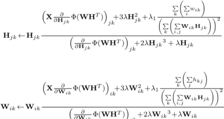
The algorithm that solve (14), called Constraint Post Non-Linear Penalty Function algorithm (C-PNL-PF), is similar to the PNL-PF algorithm except for the update rules step. Thus, in C-PNL-PF, the update rule of W and H are given by:

Hjk Hjk ⇣ X_@H@ jk (WH T₎⌘ jk+3λH 2 jk+λ1 P k P i wik ! P k P i,jWikHjk !!2 ⇣ @ @Hjk (WH T₎⌘ jk+2λHjk 3_{+ λH} jk Wik Wik ⇣ X_@W@ ik (WH T₎⌘ ik+3λW 2 ik+λ1 P k P jhkj ! P k P i,j WikHjk !!2 ⇣ @ @Wik (WH T₎⌘ jk+2λWik 3_+λW ik

In the next section, the different models and algorithms presented in this paper are compared in numerical simulations.

V. NUMERICAL SIMULATIONS

In this section, we compare the two BMF algorithms pre-sented in [18] based on linear mixture model (3) (PF and TH) and the two proposed algorithms based on the post nonlinear model (10) (PNL-PF and C-PNL-PF).

A first experiment compares the different algorithms in the case of K=2 uncorrelated sources, i.e., sources having dis-joint supports. One can observe that, all algorithms estimate correctly X, W and H (figure 1), as in this case, models (1), (3) and (10) are equivalent. In the second experiment, we have two sources strongly correlated in the identifiable case

i.e., each source verify theorem III.1. We can see that, the

TH algorithm does not estimate correctly the matrices, the PF algorithm estimates well W and H but the reconstructed X is not accurate. This is because the direct model (3) used in these algorithms is not equivalent to the original BMF model (1) when the sources are correlated. On the other hand, the two proposed algorithms estimate well X, W and H (figure 2). The third experiment compares the PF, PNL-PF and C-PNL-PF algorithms in the case of 3 correlated sources. This mixture is not identifiable because the second source (X2= w2� hT2)

do not verify the condition of theorem III.1. We can observe that, the PF algorithm fails completely. The PNL-PF algorithm estimates well X and H but not W (figure 3). Actualy, as the model is not identifiable, the PNL-PF algorithm finds another admissible solution. The C-PNL-PF algorithm allows to find the right solution of H, W and X.

50 100 150 X initial 20 40 60 80 100 120 0 1 2 W initial 0 50 100 0 1 2 H initial 0 50 100 150 50 100 150 X TH reconstructed 20 40 60 80 100 120 0 1 2 W TH estimated 0 50 100 0 1 2 H TH estimed 0 50 100 150 50 100 150 X PF reconstructed 20 40 60 80 100 120 0 1 2 W PF estimated 0 50 100 0 1 2 H PF estimed 0 50 100 150 50 100 150 X PNL-PF reconstructed 20 40 60 80 100 120 0 1 2 W PNL-PF estimated 0 50 100 0 1 2 H PNL-PF estimed 0 50 100 150 50 100 150 X C-PNL-PF reconstructed 20 40 60 80 100 120 0 1 2 W C-PNL-PF estimated 0 50 100 0 1 2 H C-PNL-PF estimed 0 50 100 150

Figure 1:Comparison of TH, PF, PNL-PF and C-PNL-PF algorithms for the case of two uncorrelated sources (N=120, M=150, γ = 150, λ= 800, λ1= 107) 50 100 150 X initial 20 40 60 80 100 120 0 1 2 W initial 0 50 100 0 1 2 H initial 0 50 100 150 50 100 150 X TH reconstructed 20 40 60 80 100 120 0 1 2 W TH estimated 0 50 100 0 1 2 H TH estimed 0 50 100 150 50 100 150 XPF reconstructed 20 40 60 80 100 120 0 1 2 WPF estimated 0 50 100 0 1 2 HPF estimed 0 50 100 150 50 100 150 X PNL-PF reconstructed 20 40 60 80 100 120 0 1 2 W PNL-PF estimated 0 50 100 0 1 2 H PNL-PF estimed 0 50 100 150 50 100 150 X C-PNL-PF reconstructed 20 40 60 80 100 120 0 1 2 W C-PNL-PF estimated 0 50 100 0 1 2 H C-PNL-PF estimed 0 50 100 150

Figure 2:Comparison of TH, PF, PNL-PF and C-PNL-PF algorithms for the case of two correlated sources (N=120, M=150, γ = 150, λ = 800, λ1= 107) 50 100 150 X initial 20 40 60 80 100 120 0 1 2 3 W initial 0 50 100 0 1 2 3 H initial 0 50 100 150 50 100 150 X PF reconstructed 20 40 60 80 100 120 0 1 2 3 W PF estimated 0 50 100 0 1 2 3 H PF estimed 0 50 100 150 50 100 150 X PNL-PF reconstructed 20 40 60 80 100 120 0 1 2 3 W PNL-PF estimated 0 50 100 0 1 2 3 H PNL-PF estimed 0 50 100 150 50 100 150 X C-PNL-PF reconstructed 20 40 60 80 100 120 0 1 2 3 W C-PNL-PF estimated 0 50 100 0 1 2 3 H C-PNL-PF estimed 0 50 100 150

Figure 3:Comparison of PF, PNL-PF and C-PNL-PF algorithms for the case of 3 correlated sources (N=120, M=150, γ = 150, λ =800, λ1 =2 · 108)

The second part of this section aims at evaluating the statiscal performance of these algorithms. We consider a rank

5 BMF model where each column of W and H follows a Bernoulli distribution of parameter b (%) which represents the probability of non-zero elements. The quality of estimation is assessed by the error rate in the estimation of the columns of W and H (mean, [min, max]) obtained by averaging the result over 100 trials of the Bernoulli random variables. When the Bernoulli parameter is low, the sources correlation (overlapping) is low. When b increases, the sources correlation increases.

Results reported in table I, correspond to b = 30% which result in binary sources weakly correlated. In that case, all the algorithms yield a low error rate (< 1%) but only PNL-PF and C-PNL-PF yield an error rate equal to 0% which shows that in that case, the identifiability condition was verified. This is no longer true when b increases; in that case only C-PNL-PF gives low error rate (table II).

X W H

TH 0.99 [0.48 1.6] 0.3 [0 1.0] 0.45 [0 1.2]

PF 0.13 [0 0.68] 0.13 [0 0.66] 0 [0 0]

PNL-PF 0 [0 0] 0 [0 0] 0 [0 0]

C-PNL-PF 0 [0 0] 0 [0 0] 0 [0 0]

Table I:The mean, minimum and maximum of the estimation error rate of Wand H columns and X sources for b = 30%(N=120, M=150, γ = 170,

λ=800, λ1= 100) X W H TH 20.7 [3.4 37.2] 5.65 [0.4 10.8] 3.64 [0.1 8.3] PF 19.3 [6.7 36.2] 5.74 [0.9 11.4] 3.2 0[.04 8.3] PNL-PF 12.6 [1.1 32.2] 3.40 [0.05 9.1] 2.1 [0.0 7.3] C-PNL-PF 4.3[0.1 13.7] 1.86 [0.9 3.9] 1.5 [0.8 3.5]

Table II:The mean, minimum and maximum of the estimation error rate of Wand H columns and X sources for b = 55%(N=120, M=150, γ = 170,

λ=800, λ1= 108)

VI. CONCLUSION

In this paper we studied the identifiability of the binary mixture model and provided a necessary and sufficient identi-fiability condition. We also introduced a novel post nonlinear mixture model which is equivalent to the binary mixture model when the matrices are strictly binary. Based on this model, two algorithms for binary matrix factorization have been proposed and their performance has been compared in simulations to two state of the art methods. Our approach gives more accurate estimates of the binary matrices, especially when the columns of the matrices are highly correlated.

Future work will study the robustness of the proposed algo-rithms to binary noise and how to optimally choose the value of the hyper parameters.

REFERENCES

[1] Radim Belohlavek, Cynthia Glodeanu, and Vilem Vychodil. Optimal factorization of three-way binary data using triadic concepts. Order, 30(2):437–454, 2013.

[2] Radim Belohlavek and Vilem Vychodil. Discovery of optimal factors in binary data via a novel method of matrix decomposition. Journal of

Computer and System Sciences, 76(1):3–20, 2010.

[3] Daizhan Cheng, Yin Zhao, and Xiangru Xu. Matrix approach to boolean calculus. In Decision and Control and European Control Conference

(CDC-ECC), 2011 50th IEEE Conference on, pages 6950–6955. IEEE,

2011.

[4] Peng Jiang and M Heath. Mining discrete patterns via binary matrix factorization. In Data Mining Workshops (ICDMW), 2013 IEEE 13th

International Conference on, pages 1129–1136. IEEE, 2013.

[5] Mehmet Koyut¨urk, Ananth Grama, and Naren Ramakrishnan. Algebraic techniques for analysis of large discrete-valued datasets. In European

Conference on Principles of Data Mining and Knowledge Discovery,

pages 311–324. Springer, 2002.

[6] Mehmet Koyuturk, Ananth Grama, and Naren Ramakrishnan. Com-pression, clustering, and pattern discovery in very high-dimensional discrete-attribute data sets. IEEE Transactions on Knowledge and Data

Engineering, 17(4):447–461, 2005.

[7] Daniel D Lee and H Sebastian Seung. Learning the parts of objects by non-negative matrix factorization. Nature, 401(6755):788–791, 1999. [8] Daniel D Lee and H Sebastian Seung. Algorithms for non-negative

matrix factorization. In Advances in neural information processing

systems, pages 556–562, 2001.

[9] Tao Li. A general model for clustering binary data. In Proceedings

of the eleventh ACM SIGKDD international conference on Knowledge discovery in data mining, pages 188–197. ACM, 2005.

[10] R Duncan Luce. A note on boolean matrix theory. Proceedings of the

American Mathematical Society, 3(3):382–388, 1952.

[11] Edward Meeds, Zoubin Ghahramani, Radford M Neal, and Sam T Roweis. Modeling dyadic data with binary latent factors. In Advances

in neural information processing systems, pages 977–984, 2006.

[12] Pauli Miettinen, Taneli Mielikainen, Aristides Gionis, Gautam Das, and Heikki Mannila. The discrete basis problem. Knowledge and Data

Engineering, IEEE Transactions on, 20(10):1348–1362, 2008.

[13] Elena Nenova, Dmitry I Ignatov, and Andrey V Konstantinov. An fca-based boolean matrix factorisation for collaborative filtering. arXiv

preprint arXiv:1310.4366, 2013.

[14] Bao-Hong Shen, Shuiwang Ji, and Jieping Ye. Mining discrete patterns via binary matrix factorization. In Proceedings of the 15th ACM

SIGKDD international conference on Knowledge discovery and data mining, pages 757–766. ACM, 2009.

[15] Shikui Tu, Runsheng Chen, and Lei Xu. A binary matrix factorization algorithm for protein complex prediction. Proteome Science, 9(1):1, 2011.

[16] Arie Yeredor. Ica in boolean xor mixtures. In Independent Component

Analysis and Signal Separation, pages 827–835. Springer, 2007.

[17] Zhong-Yuan Zhang, Tao Li, Chris Ding, Xian-Wen Ren, and Xiang-Sun Zhang. Binary matrix factorization for analyzing gene expression data.

Data Mining and Knowledge Discovery, 20(1):28–52, 2010.

[18] Zhongyuan Zhang, Chris Ding, Tao Li, and Xiangsun Zhang. Binary matrix factorization with applications. In Data Mining, 2007. ICDM

2007. Seventh IEEE International Conference on, pages 391–400. IEEE,