HAL Id: pasteur-03037346
https://hal-pasteur.archives-ouvertes.fr/pasteur-03037346
Submitted on 3 Dec 2020HAL is a multi-disciplinary open access
archive for the deposit and dissemination of sci-entific research documents, whether they are pub-lished or not. The documents may come from teaching and research institutions in France or abroad, or from public or private research centers.
L’archive ouverte pluridisciplinaire HAL, est destinée au dépôt et à la diffusion de documents scientifiques de niveau recherche, publiés ou non, émanant des établissements d’enseignement et de recherche français ou étrangers, des laboratoires publics ou privés.
Sparse Multiple Correspondence Analysis
Vincent Guillemot, Julie Le Borgne, Arnaud Gloaguen, Arthur Tenenhaus,
Gilbert Saporta, Sylvie Chollet, Derek Beaton, Hervé Abdi
To cite this version:
Vincent Guillemot, Julie Le Borgne, Arnaud Gloaguen, Arthur Tenenhaus, Gilbert Saporta, et al.. Sparse Multiple Correspondence Analysis. 52èmes Journées de Statistique, May 2020, Nice, France. �pasteur-03037346�
Sparse Multiple Correspondence Analysis
Vincent Guillemot1,⇤, Julie Le Borgne1, Arnaud Gloaguen2, Arthur Tenenhaus2, Gilbert
Saporta3, Sylvie Chollet4, Derek Beaton5, Herv´e Abdi6,⇤
1 Bioinformatics/Biostatistics Hub, CBD, Institut Pasteur, USR 3756 CNRS, Paris, FR 2 Laboratoire des Signaux et Syst`emes, CentraleSupelec, Gif-Sur-Yvette, FR
3 CEDRIC, Conservatoire National des Arts et M´etiers, Paris, FR 4 Institut Sup´erieur d’Agriculture de Lille, Lille, FR
5 The Rotman Institute at Baycrest, Toronto, Canada 6 The University of Texas at Dallas, Richardson, TX, USA
⇤ E-mail: [email protected], [email protected]
R´esum´e. L’Analyse des Correspondances Multiples (ACM) est la m´ethode de choix pour l’analyse des donn´ees cat´egorielles multivari´ees. Bas´ee sur la d´ecomposition en valeurs singuli`eres (SVD), l’ACM b´en´eficie naturellement des extensions de cette derni`ere, dont celles qui permettent de r´ealiser des analyses parcimonieuses. L’algorithme permet-tant de r´ealiser l’ACM parcimonieuse n´ecessite deux propri´et´es particuli`eres addition-nelles: l’inclusion des matrices de m´etriques (masses et poids) caract´eristiques de l’ACM, et la possibilit´e de s´electionner des groupes entiers de variables (un groupe ´etant constitu´e du codage disjonctif complet d’une variable cat´egorielle). Nous proposons un algorithme pour l’ACM parcimonieuse bas´e sur la d´ecomposition en valeurs singuli`eres g´en´eralis´ee et une projection sur la boule `1,2. Nous illustrons notre m´ethode avec les r´esultats d’une
enquˆete par questionnaires sur les connaissances alimentaires et la perception de fromages. Mots-cl´es. Parcimonie, Analyse Multivari´ee, Analyse des Correspondances Multiples Abstract. Multiple Correspondence Analysis (MCA) is the method of choice for the multivariate analysis of categorical data. In MCA each qualitative variable is represented by a group of binary variables (with a coding scheme called “complete disjunctive coding”) and each binary variable has a weight inversely proportional to its frequency. The data matrix concatenates all these binary variables, and once normalized and centered this data matrix is analyzed with a generalized singular value decomposition (GSVD) that incorporates the variable weights as constraints (or “metric”). The GSVD is, of course, based on the plain SVD and so MCA can be sparsified by extending algorithms designed to sparsify the SVD. To do so requires two additional features: to include weights and to be able to sparsify entire groups of variables at once. Another important feature of such a sparsification should be to preserve the orthogonality of the components, Here, we integrate all these constraints by using an exact projection scheme onto the intersection of subspaces (i.e., balls) where each ball represents a specific type of constraints. We illustrate our procedure with the data from a questionnaire survey on the perception of cheese in two French cities.
Keywords. Sparsity, Multivariate Analysis, Multiple Correspondence Analysis
1
a
Akin to principal component analysis (PCA), Multiple Correspondence Analysis (MCA, see for reviews [1, 6, 8]) is a multivariate analysis method that analyzes the structure of a set of I observations described by K qualitative variables each comprising Jk modalities.
In MCA, the response of an observation to a qualitative variable is represented by a binary vector. The I by J data matrix to analyze (denoted Y), called the disjunctive table, is the concatenation of K matrices each with I observations and Jk columns. In MCA, the
matrix actually analyzed is the centered probability matrix denoted X, and computed as X = Y⇥ (IK)−1− rc> with r = Y1 ⇥ (IK)−1 and c = Y>1 ⇥ (IK)−1 . (1) MCA is obtained from the generalized singular value decomposition (GSVD) of X as
X = P∆Q> with P>MP = Q>WQ = I where M = diag{r} and W = diag{c} (2) with the diag operator transforming a vector into a diagonal matrix. In MCA, the inter-pretation of the dimensions is greatly facilitated when variables have either a very large or a very small (rather than a medium) contribution to a given dimension. In standard PCA such a pattern is obtained by rotation of the dimensions (e.g., with VARIMAX) or by sparsification (see [5]). To extend sparsification to MCA (for previous work on Sparse MCA see [2, 7]), the procedure needs to rely on extensions of sparsification that can in-corporate 1) the constraints imposed by the matrices M and W and 2) a group constraint which imposes that the entire block of columns representing a variable is is selected or discarded by the sparsification procedure. In addition, as for standard sparsification of PCA, the interpretation of the results is improved when the sparsified dimensions are pairwise orthogonal, but previous sparsification methods for MCA do not implement the orthogonality constraint and sparsify only single variables. In this paper we present a gen-eralization of the sparsified SVD (the SGSVD) that implements all the aforementioned constraints. We first present the method as an optimization problem, derive the algo-rithm for this optimization problem, and illustrate this new method with the analysis of a questionnaire on food preference.
1
Method
The algorithm that we propose solves the following optimization problem
arg min P,∆,Q 1 2 ! !X − P∆Q> ! ! 2 2 with ( P>MP = I Q>WQ = I, and8` = 1, ..., R ( kp`kG c1,` kq`kG c2,` (3)
where k.k2 is the Euclidean norm, c1,` and c2,` are positive scalars controlling the sparsity
constraint for the pseudo-singular vectors, and where the group norm is defined as: kxkG =
PG
g=1kxιgk2. In other words, it is the `1-norm of the vector containing the `2-norm of the sub-vectors defined by the groups. The `1,2-ball associated with this norm is noted B1,2(·).
2
Data: X, ", R
Result: Sparse MCA of X Define P = 0;
Define Q = 0;
Apply weights and masses to X; for ` = 1, . . . , R do
p(0) and q(0) are randomly initialized;
δ(0)←0; δ(1)←p(0)>Xq(0); s ← 0; while$ $δ(s+1)− δ(s)$ $≥ " do p(s+1)← proj(Xq(s), B 1,2(c1,`) \ B2(1) \ P?); q(s+1) ← proj(X>p(s+1), B 1,2(c2,`) \ B2(1) \ Q?); δ(s+1) ←p(s+1)>Xq(s+1); s ← s + 1 ; end δ` ←δ(s+1); P ← vec%P, p(s+1)&; Q ← vec%Q, q(s+1)&; end
Apply inverse weights and masses to P and Q;
Algorithm 1: General algorithm of the sparse MCA.
1.1
The sparse MCA algorithm
The sparse MCA algorithm is presented in Algorithm 1. It is essentially an alternate projection algorithm. Its key component is the projection onto the intersection between the ball defined by the group constraint, the `2-ball, and the space orthogonal to the
already estimated singular triplets (left or right).
To achieve the projections on B1,2(c1,`) \ B2(1) \ P? and B1,2(c2,`) \ B2(1) \ Q?, we
perform a Projection Onto Convex Sets (POCS) [3] with two components: the projection onto the intersection of the group ball and the `2-ball, and the projection onto the
or-thogonal spaces defined by the already estimated pseudo-singular vectors. We detail the first projection in the next section.
1.2
Projection onto the intersection of the group and the `
2-balls
Here, we present a fast and exact algorithm for the projection of x, a fixed vector of Rn
that comprises K non-overlapping groups, onto the intersection of an `1,2-ball of radius c
and the `2-ball of radius 1. This generalizes the projection onto B1(c) \ B2(1) [4].
3
Denote by G the set of the indices defining the groups: G = {◆k, k = 1, ..., K}, where
◆k indicates the variables contained in group k and K is the number of groups. Let v be the vector containing all the `2-norms of the sub-vectors xιk, k = 1, ..., K. The real and positive value λ⇤ is such that k prox
λ⇤kkG(x)kG = c if and only if k proxλ⇤kk1(v)k1= c,
where proxf is the proximal operator of a convex function f . Recall that the projection onto a ball is intimately linked to the proximal operator of the ball’s norm. So, projecting x onto B1,2(c) \ B2(1) is equivalent to projecting v onto B1(c) \ B2(1), which can be
achieved with the algorithm presented in [4].
2
Results
We analyzed the answers to two sets of questions of a survey on cheese answered by a sample of French participants from the two French cities of Angers and Lille. The 8 questions from the first set evaluate knowledge with answers coded as either correct or incorrect. The 23 questions from the second set evaluate the behaviors, opinions, or attitudes of the respondents toward cheese that are either farm-made or industrial. These questions are answered with a 4 point Likert scale (from 1 meaning “I totally agree” to 4 meaning “I totally disagree”). In addition we have information about the respondents: Sex, Age (coded in 4 categories), and the city where they live (Angers or Lille).
A regular MCA was applied to this data, as well as a sparse MCA with the constraints that each dimension be based on only one group of variables (i.e., a unique categorical variable) and only one group of observations (i.e., city of origin).
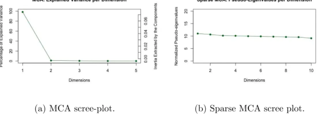
The Scree-plots on Figures 1a and 1b show that the first dimension of the regular MCA captures most of the variability of the data, whereas for the sparse MCA the pseudo-eigenvalues (normalized by the total inertia) are almost all equal.
(a) MCA scree-plot. (b) Sparse MCA scree plot.
Figure 1: Scree-plots of the regular (left) and sparse (right) MCA.
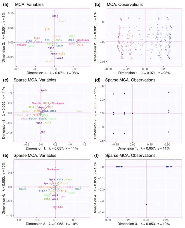
The first two dimensions obtained with the regular MCA are shown in Figures 2a and 2b that confirm that city of origin is the main source of variability from this data set.
4
The results of the sparse MCA (see Figures 2c, 2d, 2e, and 2f) reveal that: Age is an important component on the structure of the Angers group, followed by “knowledge” and gender whereas the second city of origin (Lille) is associated with the fourth dimension.
3
Conclusion
We developed a sparse version of the MCA that incorporates into the GSVD, the group constraints imposed on the different modalities of a qualitative variable, and illustrated with real data that this new approach can simplify the interpretation of the factorial dimensions as well as reveal deeper insights. Future directions will include taking into account a hierarchical structure of either variables or observations such as overlapping groups of grouped variables as can be found, for example, for SNP data structured into pathways.
References
[1] H. Abdi and D. Valentin. Multiple Correspondence Analysis. In Encyclopedia of Measurement and Statistics. SAGE Publications, Inc., Thousand Oaks, 2007.
[2] A. Bernard, C. Guinot, and G. Saporta. Sparse principal component analysis for multiblock data and its extension to sparse multiple correspondence analysis. In Pro-ceedings of 20th International Conference on Computational Statistics (COMPSTAT 2012), pages 99–106, 2012.
[3] P. Combettes. The foundations of set theoretic estimation. Proceedings of the IEEE, 81(2):182–208, 1993.
[4] A. Gloaguen, V. Guillemot, and A. Tenenhaus. An efficient algorithm to satisfy `1
and `2 constraints. In 49`emes Journ´ees de statistique, Avignon, France, 2017.
[5] V. Guillemot, D. Beaton, A. Gloaguen, T. L¨ofstedt, B. Levine, N. Raymond, A. Tenen-haus, and H. Abdi. A constrained singular value decomposition method that integrates sparsity and orthogonality. PLOS ONE, 14(3):e0211463, mar 2019.
[6] B. Le Roux and H. Rouanet. Multiple Correspondence Analysis. Sage, Thousand Oaks, CA, 2010.
[7] Y. Mori, M. Kuroda, and N. Makino. Sparse Multiple Correspondence Analysis. In Nonlinear Principal Component Analysis and Its Applications, chapter 5, pages 47–56. Springer Singapore, 2016.
[8] G. Saporta. Probabilit´es, Analyse des Donn´ees et Statistique. Technip, Paris, France, 3rd edition, 2011.
5
Sex.f Sex.m Age.1 Age.3 Age.4 Age.2 City.Angers City.Lille Know.2 Know.1 Know.3 C01.2 C01.1 C05.1 C05.2 C07.2 C07.1 C10.1 C10.2 C11.2 C11.1 C18.2 C18.1 −0.05 0.00 0.05 0.10 −0.6 −0.3 0.0 0.3 Dimension 1. λ = 0.071. τ = 98% Dimension 2 . λ = 0.001 . τ = 1 % MCA. Variables (a) −0.05 0.00 0.05 −0.50 −0.25 0.00 0.25 Dimension 1. λ = 0.071. τ = 98% Dimension 2 . λ = 0.001 . τ = 1 % MCA. Observations (b) Sex.f Sex.m Age.1 Age.3 Age.4 Age.2 City.Angers City.Lille Know.2 Know.1 Know.3 C01.2 C01.1 C05.1 C05.2 C07.2 C07.1 C10.1 C10.2 C11.2 C11.1 C18.2 C18.1 −1.0 −0.5 0.0 0.5 1.0 −0.5 0.0 0.5 1.0 1.5 Dimension 1. λ = 0.057. τ = 11% Dimension 2 . λ = 0.055 . τ = 11 %
Sparse MCA. Variables
(c) −0.6 −0.3 0.0 0.3 0.6 −0.25 0.00 0.25 0.50 Dimension 1. λ = 0.057. τ = 11% Dimension 2 . λ = 0.055 . τ = 11 %
Sparse MCA. Observations
(d) Sex.f Sex.m Age.1 Age.3 Age.4 Age.2 City.Angers City.Lille Know.2 Know.1 Know.3 C01.2 C01.1 C05.1 C05.2 C07.2 C07.1 C10.1 C10.2 C11.2 C11.1 C18.2 C18.1 −1.0 −0.5 0.0 0.5 −1.0 −0.5 0.0 0.5 Dimension 3. λ = 0.053. τ = 10% Dimension 4 . λ = 0.053 . τ = 10 %
Sparse MCA. Variables
(e) −0.4 −0.3 −0.2 −0.1 0.0 −0.50 −0.25 0.00 0.25 Dimension 3. λ = 0.053. τ = 10% Dimension 4 . λ = 0.053 . τ = 10 %
Sparse MCA. Observations
(f)
Figure 2: Variable and observation maps for MCA and sparse MCA. Only Dimensions 1 and 2 are shown for the regular MCA. For the sparse MCA, we show Dimensions 1 and 2 (middle figures) and Dimensions 3 and 4 (lower figures).
6