Filtering Relocations on a Delaunay Triangulation

HAL Id: inria-00413344

https://hal.inria.fr/inria-00413344

HAL is a multi-disciplinary open access archive for the deposit and dissemination of sci-entific research documents, whether they are pub-lished or not. The documents may come from

L’archive ouverte pluridisciplinaire HAL, est destinée au dépôt et à la diffusion de documents scientifiques de niveau recherche, publiés ou non, émanant des établissements d’enseignement et de

Filtering Relocations on a Delaunay Triangulation

Pedro Machado Manhães de Castro, Jane Tournois, Pierre Alliez, Olivier

Devillers

To cite this version:

Pedro Machado Manhães de Castro, Jane Tournois, Pierre Alliez, Olivier Devillers. Filtering Re-locations on a Delaunay Triangulation. Computer Graphics Forum, Wiley, 2009, �10.1111/j.1467-8659.2009.01523.x�. �inria-00413344�

Filtering Relocations on a Delaunay Triangulation

Pedro Machado Manhães de Castro Jane Tournois Pierre Alliez

Olivier Devillers

INRIA Sophia Antipolis - Méditerranée, France September 3, 2009

Abstract

Updating a Delaunay triangulation when its vertices move is a bottle-neck in several domains of application. Rebuilding the whole triangulation from scratch is surprisingly a very viable option compared to relocating the vertices. This can be explained by several recent advances in efficient con-struction of Delaunay triangulations. However, when all points move with a small magnitude, or when only a fraction of the vertices move, rebuilding is no longer the best option. This paper considers the problem of efficiently updating a Delaunay triangulation when its vertices are moving under small perturbations. The main contribution is a set of filters based upon the concept of vertex tolerances. Experiments show that filtering relocations is faster than rebuilding the whole triangulation from scratch under certain conditions.

Classification:Computer Graphics, I.3.5, Computational Geometry and Object Modeling: Geometric algorithms, languages, and systems

1

Introduction

Delaunay triangulation of a point set is one of the most famous and successful data structures introduced in the field of Computational Geometry. Two main reasons explain this success. First, it is suitable to many practical uses such as mesh gen-eration for finite elements methods [Ede01] or surface reconstruction from point sets [CG06]. Second, computational geometers have produced efficient implemen-tations [BDP∗_{02, She96].}

In several applications, the triangulation needs to evolve over time. Thus, the vertices of the triangulation - defined by input data points - are moving. This hap-pens for instance in data clustering [HW79, AV07], mesh generation [DBC07], re-meshing [VCP08,ACD∗_{03], mesh smoothing [ABE97], mesh optimization [ACYD05,}

The Delaunay triangulation of a set S of n points in Rd_{is a simplicial complex.}

It is defined such that no point in S is inside the circumsphere of any simplex in the Delaunay triangulation [PS90, Aur91]. Several Delaunay triangulation algorithms have been described in the literature. Many of them are appropriate in the static setting [SH75, For87], where the points are fixed and known in advance. There is also a variety of so-called dynamic algorithms [GS78, Dev02, DLM04], in which the points are fixed and the triangulation is maintained under point insertions or deletions. Next, if some of the points move continuously and we want to keep track of all topological changes, we are dealing with kinetic algorithms [Gui98, Rus07]. Finally, an important variant occurs when the points move and when we are only interested in the triangulation at some discrete timestamps. We call such context timestamp relocation.

Notions. In the context of timestamp relocation, a simple method consists of rebuilding the whole triangulation from scratch at every timestamp. We denote by rebuildingsuch approach. When the output has an expected linear size, rebuilding can lead to a O(knlog(n)) time complexity, where n denotes the number of vertices of the triangulation and k denotes the number of distinct timestamps. Despite its poor theoretical complexity, the rebuilding algorithm turns out to be surprisingly hard to outperform when most of the points move, as already observed [Rus07]. Rebuilding the triangulation from scratch allows using the most efficient static algorithms. In this paper we use the Delaunay triangulations from the CGAL li-brary [Yvi08,PT08]. The latter sort the points so as to best preserve point proximity for efficient localization, and make use of randomized incremental constructions.

There are a number of applications which require computing the next ver-tex locations one by one, updating the Delaunay triangulation after each reloca-tion [ACYD05,TAD07,TWAD09]. Naturally, rebuilding is unsuitable for such ap-plications. Another naive updating algorithm, significantly different from rebuild-ing, is the relocation algorithm, which relocates the vertices one by one. Roughly speaking, the latter consists of iterating over all vertices to be relocated. For each relocated vertex the algorithm first walks through the triangulation to locate the simplex containing its new position, inserts a vertex at the new position and re-moves the old vertex from the triangulation. This way each relocation requires three operations for each relocated point: one point location, one insertion and one removal. When the displacement of a moving point is small enough the point loca-tion operaloca-tion is usually fast. In favorable configuraloca-tions with small displacement and constant local triangulation complexity, the localization, insertion, and dele-tion operadele-tions take constant time per point. This leads to O(m) complexity per timestamp, where m is the number of moving points. Such complexity is theoreti-cally better than the O(nlogn) complexity of rebuilding. In practice however, the deletion operation is very costly and hence rebuilding the whole triangulation is

faster when all vertices are relocated, i.e., when m = n.

Algorithms which are not able to relocate vertices one by one are referred to as static. Algorithms relocating vertices one by one are referred to as dynamic. Advantages of being dynamic include to name a few:

–1– the computational complexity depends mostly on the number of moving points (which impacts on applications where points eventually stop moving);

–2– the new location of a moving point can be computed on-line which is required for variational methods [DBC07, ACYD05, TAD07, TWAD09];

–3– the references to the memory that the user may have remain valid (conversely to rebuilding).

Rebuilding is static while the relocation algorithm is dynamic.

Previous Work. Several recent approaches have been proposed to outperform the two naive algorithms (rebuilding and relocation) in specific circumstances. For example, kinetic data structures [Gui98] are applicable with a careful choice of vertex trajectories [Rus07]. Some work has also been done to improve the way ki-netic data structures handle degeneracies [ABTT08]. Approaches based on kiki-netic data structuresare often dynamic as they can relocate one vertex at a time. Guibas and Russel consider another approach [GR04] which consists of the following se-quence: Remove some points until the triangulation has a non overlapping embed-ding, flip the invalid pairs of adjacent simplices until the triangulation is valid (i.e., Delaunay), and add insert back the previously removed points. In this approach the flipping step may lead to deadlocks in dimensions higher than two, which trigger rebuildings from scratch with huge computational overhead. For their input data however, deadlocks do not happen so often and rebuilding can be outperformed when considering heuristics on the ordering of the points to be removed. Although this method is dynamic when relocating one vertex at a time, it loses consider-ably its efficiency as it is not allowed to use any heuristic anymore in this case. Shewchuk proposes two elegant algorithms to repair Delaunay triangulations: star splaying and star flipping [She05]. Both algorithms can be used when flipping causes a deadlock, instead of rebuilding the triangulation from scratch. Finally, for applications which can live with triangulations which are not necessarily De-launay at every timestamp (e.g., almost-DeDe-launay upon lazy removals [DBC07]), some dynamic approaches outperform rebuilding by a factor of three [DBC07]. It is worth mentioning that dynamic algorithms, which perform nearly as fast as rebuilding, are also very well-suited to applications based on variational methods.

Contributions. We propose to compute for each vertex of the triangulation a safety zone where the vertex can move without changing its connectivity. This way each relocation which does not change the connectivity of the triangulation is filtered. We show experimentally that this approach is worthwhile for applications where the points are moving under small perturbations.

Our main contribution takes the form of a filtering method for relocating the points of a Delaunay triangulations when the points move with small amplitude. The noticeable advantages of the filter are: –1– Simplicity. The implementation is simple as it relies on well-known dynamic Delaunay triangulation construc-tions [Dev02, DLM04] with few additional geometric computaconstruc-tions; and –2– Effi-ciency.Our filtering approach outperforms in our experiments by at least a factor of four, in two and three dimensions, the current dynamic relocation approach used in mesh optimization [TAD07]. It also outperforms the rebuilding algorithm for sev-eral conducted experiments. This opens new perspectives for sevsev-eral applications. For example, in mesh optimization, the number of iterations is shown to impact the mesh quality under converging schemes. The proposed algorithm enables the possibility of going further on the number of iterations while being dynamic.

2

Fundamentals

We now review the necessary background on Delaunay triangulations and intro-duce the notions of safe region and tolerance region of a vertex.

2.1 Certificates and Tolerances

A predicate is a function on a set of primitives which returns one value in a discrete set of possible results. In this paper, we consider the common case where we compute a numerical value denoted by predicate discriminant: the result of the predicate is the sign of this value. When one or more predicates are used to evaluate whether a geometric data structure is valid or invalid, we denote by certificate each of those predicates. In the sequel a certificate is said to be valid when it is positive. Let C : Am_{→ {−1, 0, 1} be a certificate, acting on a m-tuple of points ζ =}

(z1, z2, . . . , zm) ∈ Am, where A is the space where the points lie. By abuse of

notation, z ∈ ζ means that z is one of the points of ζ. We define the tolerance of ζ with respect to C, namely εC(ζ) or simply ε(ζ) when there is no ambiguity, the

largest displacement applicable to z ∈ ζ without invalidating C. More precisely, the tolerance, assuming C(ζ) > 0, can be stated as follows:

εC(ζ) = inf ζ′ C(ζ′)≤0 distH(ζ, ζ ′ ), (1)

where distH(ζ, ζ′) is the Hausdorff distance between two finite sets of points.

Let X be a finite set of m-tuples of points in Am_{. Then, the tolerance of an}

Cand to X , is denoted εC,X(e) (or simply by ε(e) when there is no ambiguity). It is defined as follows: εC,X(e) = inf ζ∋e ζ∈X εC(ζ). (2)

2.2 Delaunay Triangulations: Certificate and Tolerance

An intersection free triangulation lying in Rd_{can be checked to be Delaunay using}

the empty-sphere certificate [DLPT98]. This certificate states that, for each facet of the triangulation, the hypersphere passing through the d + 1 vertices of a simplex on one side does not contain the vertex on the other side. Therefore, this certificate is applied to any d + 2 distinct points z1= (x11, . . . , x1d), . . . , zd+2= (xd+21 , . . . , xd+2d )

of the triangulation which belong to the same pair of incident cells. In the sequel, such a pair is called a bi-cell (see Figure 1).

The tolerance involved in a Delaunay triangulation is the tolerance of the empty-sphere certificateacting on any bi-cell of a Delaunay triangulation. From Equa-tion 1, it corresponds to the size of the smallest perturbaEqua-tion the bi-cell’s vertices can undergo so as to become cospherical. This is equivalent to compute the hyper-sphere that minimizes the maximum distance to the d + 2 vertices, i.e., the optimal middle sphere, which is the median sphere of the d-annulus of minimum width containing the vertices. An annulus, defined as the region between two concentric hyperspheres, is a fundamental object in Computational Geometry [GLR97]).

Dealing with Boundary. In the following we use a simple way to deal with the boundary of the triangulation (i.e., its convex hull) by adding a “point at infinity” ∞ to the initial set of points [AGMR98,Yvi08,PT08]. Let S be the initial set of points. We consider an augmented set S′

= S ∪ {∞}. Let CH(S) be the convex hull of S and DT (S) its Delaunay triangulation, then the extended Delaunay triangulation is given by

DT(S′) = DT (S) ∪ {( f , ∞) | f facet of CH(S)}. (3) In addition to DT (S), every point on the boundary of the convex hull CH(S) is connected to ∞ creating new simplices: the infinite simplices. In contrast with DT(S), DT (S′

) has the nice property that there are exactly d + 1 simplices adjacent to each simplex in DT (S′

). This greatly simplifies the following descriptions. When dealing with infinite bi-cells, namely the ones which include the point at infinity, the d-annulus of minimum width becomes the region between two parallel hyperplanes. This happens because the hypersphere passing through ∞ reduces to an hyperplane.

In order to precise which are those parallel hyperplanes, we consider two dis-tinct cases (which coincide in two-dimensions):

(a) (b) (c)

(d) (e)

Figure 1: Definitions. (a) A three-dimensional bi-cell, (b) its interior facet and (c) opposite vertices. (d) The boundaries of its 3-annulus of minimum width; the smallest boundary passing through the facet vertices and the biggest boundary passing through the opposite vertices. (e) depicts its standard delimiter separating the facet and opposite vertices.

• If only one cell of the bi-cell is infinite then one hyperplane H1 passes

through the d common vertices of the two cells. The other hyperplane H2is

parallel to H1and passes through the unique vertex of the finite cell which is

not contained in the infinite cell (see Figure 2a).

• Otherwise the two vertices which are not shared by each cell form a line L and the remaining finite vertices are a ridge of the convex hull H (an edge in three-dimensions). Consider the hyperplanes H1 passing through H and

parallel to L and H2passing through L and parallel to H. They compose the

boundary of the d-annulus (see Figure 2b).

2.3 Tolerance Regions

Let T be a triangulation lying in Rd_{and B a bi-cell in T . The interior facet of B is}

(a) (b)

Figure 2: Infinite bi-cells. The 3-annulus of minimum-width of a bi-cell contain-ing: (a) one infinite cell and one finite cell, (b) two infinite cells.

two vertices that do not belong to its interior facet. We associate to each bi-cell B an arbitrary hypersphere S denoted by delimiter of B, see Figure 1. If the interior facet and opposite vertices of B are respectively inside and outside the delimiter of B, we say that B verifies the safety condition. We call B a safe bi-cell. If a vertex zbelongs to the interior facet of B, then the safe region of z with respect to B is the region inside the delimiter. Otherwise, the safe region of z with respect to B is the region outside the delimiter. The intersection of the safe regions of z with respect to each one of its adjacent bi-cells is called safe region of z. If all bi-cells of T are safe bi-cells we call T a safe triangulation. When a triangulation is a safe triangulation we say that it verifies the safety condition.

It is clear that a safe triangulation is equivalent to a Delaunay triangulation as: • Each delimiter can be shrunk so as to touch the vertices of the interior facet, and thus defines an empty-sphere passing through the interior facet of its bi-cell (which proves that the facets belongs to the Delaunay triangulation). • The empty-sphere property of the Delaunay triangulation facets defines

it-self empty-spheres passing through the interior facets of the bi-cells. Those empty-spheres are delimiters.

Let T be a triangulation. We define the graph (V,E) of T , where V and E are the set of vertices and edges of T respectively, as the combinatorics of T . Then we have the following proposition:

Proposition 1 Given the combinatorics of a Delaunay triangulation T , if its ver-tices move inside their safe regions, then the triangulation obtained while keeping the same combinatorics as in T in the new embedding remains a Delaunay trian-gulation.

Proposition 1 is a direct consequence of the equivalence between safe and Delau-nay triangulations: If the vertices remain inside their safe regions then T remains

Figure 3: Safe region and tolerance region. z ∈ R2_{the center of B. The region A}

is the safe region of z, while B is its tolerance region.

a safe triangulation. As a consequence it remains a Delaunay triangulation. Note that the safe region of a vertex depends on the choice of delimiters, i.e., one for each bi-cell of the triangulation. We denote by tolerance region of z, given a choice of delimiters, the biggest ball centered at the location of z included in its safe region. More precisely, let D(B) be the delimiter of a given bi-cell B. Then, for a given vertex z ∈ T , the tolerance region of z is given by:

˜ε(z) = inf

B∋z

B∈T

distH(z, D(B)). (4)

We have ˜ε(z) ≤ ε(z), since the delimiter generated by the minimum-width d-annulus of the vertices of a bi-cell B maximizes the minimum distance of the vertices to the delimiter (see Figure 3).

Among all possible delimiters of a bi-cell, we define the standard delimiter as the median hypersphere of the d-annulus with the inner-hypersphere passing through the interior facet and the outer-hypersphere passing through the oppo-site vertices. Both median hypersphere and d-annulus are unique. We call the d-annulus the standard annulus. If our choice of delimiter for each bi-cell of T is the standard delimiter, then we have ˜ε(z) = ε(z). Notice that the standard annulus is usually the annulus of minimum-width described in Section 2.2 defined by the vertices of B. In the pathological cases where the minimum-width annulus is not the standard annulus, then the standard delimiter is not safe [GLR97].

Computing the standard annulus of a given bi-cell B requires computing the center of a d-annulus. This is achieved through finding the line perpendicular to the interior facet passing through its circumcenter (it corresponds to the intersection of the bisectors of the interior facet vertices of B) and intersecting it with the bisector of the opposite vertices of B.

3

Filtering Relocations

As a remainder, the dynamic relocation algorithm which relocates one vertex after another unlike rebuilding, can be used when there is no a priori knowledge about the new point locations of the whole set of vertices. Such approach is especially useful for algorithms based on variational methods, such as [DBC07, ACYD05, TAD07, TWAD09].

In this section we propose two improvements over the naive relocation algo-rithm for the case of small displacements. Finally, we detail an algoalgo-rithm devised to filter relocations using the tolerance region of a vertex in a Delaunay triangulation (see Section 2.3). It is worth mentioning that this algorithm can be easily modified so as to incorporate other kinds of filters such as the safe region of a vertex.

3.1 Improving the Relocation Algorithm for Small Displacements

In two-dimensions a small modification of the relocation algorithm leads to a sub-stantial acceleration, by a factor of two in our experiments. This modification con-sists of flipping edges when a vertex displacement does not invert the orientation of any of its adjacent triangles. The key idea is to avoid as many removal opera-tions as possible, as they are the most expensive. In three-dimensions, repairing the triangulation is far more involved [She05].

A weaker version of this improvement consists of using relocation only when at least one topological modification is needed; otherwise the vertex coordinates are simply updated. Naturally, this additional computation leads to an overhead, though our experiments show that it pays off when displacements are small enough. When this optimization is combined with the algorithms described next, our exper-iments show evidence that it is definitely a good option.

3.2 Filtering Algorithm

We now redesign the relocation algorithm so as to take into account the tolerance region of every relocated vertex. The proposed algorithm, denoted by filtering algorithm, is capable of correctly deciding whether or not a vertex displacement requires an update of the connectivity so as to trigger the trivial update condition. It is dynamic in the sense that it preserves all benefits from the relocation algorithm compared to rebuilding.

Data structure. Consider a triangulation T , where to each vertex z ∈ T we associate two point locations: fzand mz. We denote them respectively by the fixed

and the moving position of a vertex. The fixed position is used to fix a reference position for a moving point. The moving position of a given vertex is its actual

position, and changes at every relocation. Initially the fixed and moving positions are equal. We denote by Tfand Tmthe embedding of T with respect to fz and mz

respectively. For each vertex, we store two numbers: εz and Dz which represent

respectively the tolerance value of z and the distance between fzand mz.

Pre-computations. We initially compute the Delaunay triangulation T of the initial set of points S, and for each vertex we set εz = ε(z) and Dz = 0. For

a given triangulation T , the tolerance of each vertex is computed efficiently by successively computing half the width of the standard annulus of each bi-cell of T , and keeping the minimum value on each of its vertices.

The filtering algorithm performs as follows for every vertex displacement: Input: Triangulation T after pre-computations, a vertex z of T and its new

location p.

Output: T updated after the relocation of z. (mz, Dz) ← (p, dist(fz, p)) ;

if Dz<εzthen we are done;

else

insert z in a queue Q; whileQ is not empty do

remove h from the head of Q; (fh,εh, Dh) ← (mh,∞, 0) ;

update T by relocating h with the relocation algorithm; foreach new created bi-cellB do

ε′

← half the width of the standard annulus of B ; foreach vertex w∈ B do

ifεw>ε′then

εw← ε′;

ifεw< Dwtheninsert w into Q;

end end end end end

The algorithm is shown to terminate as each processed vertex z gets a new dis-placement value Dz= 0 and thus ≤ εz. At the end of this algorithm all vertices

are guaranteed to have their Dz smaller or equal than their εz. In such a situation,

from Proposition 1, Tmis the Delaunay triangulation of the points located at

mov-ing positions. The tolerance algorithm has the same complexity as the relocation algorithm. Let n be the number of vertices of T . Although in the worst case we have n relocation calls for a single call of the filtering algorithm, if all points move, the total number of calls to the relocation algorithm is reduced to at most 2n. This

is due to the fact that when a vertex is relocated its D value is set to 0.

When relocating the vertices with a convergent scheme we can run rebuilding for the first few timestamps until the points are more or less stable, then switch to the filtering algorithm. As a drawback, the algorithm is no longer dynamic during the first timestamps. We give more details on this approach in the next section.

A natural idea is to replace the tolerance test (which checks if the moving position of a vertex stays within the tolerance distance from its fixed position) by a more involved test which checks if it stays within its safe region. We could also run this safety test in case of failure of the first test but the safety test is rather involved and does not save any computation time in practice, even when using first order approximations of its computation.

Another point concerns robustness issues. Computing the tolerance values us-ing floatus-ing point computations may in some special configurations yield to round-ing errors and hence to wrong evaluation of εz. The algorithm ensures that Tf, the

embedding at fixed position, is always correct while the embedding Tmat moving

position may be incorrect. A certified correct Delaunay triangulation for Tmis

ob-tained through a certified lower bound over εz. As expected the numerical stability

of εz depends on the quality of the simplices. To explain this fact, consider the

smallest angle θ between the line perpendicular to the interior facet of a bi-cell passing through its circumcenter and the bisector of the opposite vertices, see Fig-ure 4. The numerical stability is proportional to the size of this angle. For convex bi-cells, if θ is too small, the two simplices are said to have a bad shape [CDE∗_99].

It is worth saying that the computation of εz is rather stable in the applications

which would benefit from filtering since the shape of their simplices improve over time.

θ h

l

Figure 4: Numerical stability. If the smallest angle θ between the (d − 2)-dimension flat h and the line l is too small, the simplices are badly shaped in the sense of being non isotropic.

4

Experimental Results

This section investigates through several experiments the size of the vertex toler-ances and the width of the standard annulus in two- and three-dimensions. We

discuss the performance of the rebuilding, relocation and filtering algorithms on several data sets.

We run our experiments on a Pentium 4 at 2.5 GHz with 1GB of memory, run-ning Linux (kernel 2.6.23). The compiler used is g++4.1.2; all configurations being compiled with -DNDEBUG -O2 flags (release mode with compiler optimizations enabled). CGAL 3.3.1 is used along with an exact predicate inexact construction kernel [BFG∗_{08, FT06].}

The initialization costs of the filtering algorithm accounting for less than 0.13% of the corresponding total running time of the experiments, we consider them as negligible.

4.1 Clustering

In several applications such as image compression, quadrature, and cellular biol-ogy, to name a few, the goal is to partition a set of objects into k clusters, following an optimization criterion. Usually such criterion is the squared error function. Let Sbe a measurable set of objects in A and P = {Si}k1a k-partition of S. The squared

error function associated with P is defined as:

k

∑

where µiis the centroid of Siand dist is a given distance between two objects in A.

One relevant algorithm to find such partitions is the k-means algorithm. The most common form of the algorithm uses the Lloyd iterations [Llo82,SG86,DEJ06, ORSS06]. The Lloyd iteration starts by partitioning the input domain into k arbi-trary initial sets. It then calculates the centroid of each set and constructs a new partition by associating each point to the closest centroid. The algorithm is re-peated by alternate application of these two steps until convergence.

Let S = Rd_{, dist ∈ L}2 _{and ρ a density function in R}d_{, the latter being used to}

compute centroids. The Lloyd is described as follows: First, compute the Voronoi diagram of an initial set of k random points following the distribution ρ. Next, each cell of the Voronoi diagram is integrated so as to compute its center of mass. Finally, each point is relocated to the centroid of its Voronoi cell. Note that, for each iteration, the Delaunay triangulation of the points is updated and hence each iteration is considered as a distinct timestamp.

The convergence of the point locations evolving through the Lloyd iteration is proven for d = 1 [DEJ06]. Although only weaker convergence results are known for d > 1 [SG86], the Lloyd iteration is commonly used for dimensions higher than 1 and experimentally converges to “good” point configurations.

We consider in R2_{one uniform density function (ρ}

1= 1) as well as three

non-uniform density functions: ρ2= x2+ y2, ρ3 = x2 and ρ4= sin2px2+ y2. We

apply the Lloyd iterations to obtain evenly-distributed points in accordance with the above-mentioned density functions, see Figure 5. The standard annuli widths and tolerances increase up to convergence, while the average displacement size quickly decreases, see Figure 6. In addition the number of near-degenerate cases tends to decrease along with the iterations.

(a) Uniform density: ρ = 1

(b) Non-uniform density: ρ = x2

Figure 5: Point distribution before and after Lloyd’s iteration. 1,000 points are sampled in a disc with (a) uniform density, and (b) ρ = x2_{. The point sets are}

submitted to 1,000 Lloyd iterations with their respective density function.

As shown by Figure 7 the proposed filtering algorithm outperforms both the relocation and rebuilding algorithm. When the iteration number is really high, filtering becomes several times faster than rebuilding even though being a dynamic algorithm. At this point it is worth saying that other strategies for accelerating the Lloyd algorithm, orthogonal with respect to this one, exist. We can cite, e.g., the Lloyd-Newton method, devised to reduce the overall number of iterations [DE06a, DE06b, LWL∗_08].

! "!! #!! $!! %!! &!!! '()*+(',-! !.& !." !./ !.# 0' 1) +2)*+3)4(,5)*+-6) +2)*+3)4+--75'48'9(: 9'0;5+6)<)-( (a) evolution ! !"# !"$ !"% !"& ' ()*+ ,-+./-)012'!!! ,-+./-)012'!! ,-+./-)012'! ,-+./-)012' (b) distribution

Figure 6: Statistics in 2D. Consider a disc such that the quantity representing the number of points divided by its surface is equal to 1. The square root of this quantity is the unity of distance. The curves depict for 1,000 Lloyd iterations with ρ = x2: (a) the evolution of the average displacement size, the average standard annulus width and the average tolerance of vertices; (b) the distribution of the standard annulus width for iteration 1, 10, 100 and 1,000.

0 200 400 600 800 1000 iteration 0 2 4 6 8 se co n d s filtering rebuild ing relo catio n (a) uniform (ρ = 1) 0 200 400 600 800 1000 iteration 0 2 4 6 8 se co n d s filtering

rebuilding

relo catio n (b) ρ = x2+ y2 0 200 400 600 800 1000 iteration 0 2 4 6 8 se co n d s filtering

rebuilding

relo catio n (c) ρ = x2 0 200 400 600 800 1000 iteration 0 2 4 6 8 se co n d s filtering

rebuilding

relo catio

n

(d) ρ = sin2p x2+ y2

Figure 7: Computation times in 2D. The curves depict the cumulated computation times for running up to 1,000 Lloyd’s iterations with: (a) uniform density (ρ = 1); (b) ρ = x2_{+ y}2_{; (c) ρ = x}2_{; and (d) ρ = sin}2p

x2+ y2. The filtering algorithm consistently outperforms rebuilding for every density function. Note how the slope of the filtering algorithm’s curve decreases over time.

4.2 Mesh Optimization

We choose as experiment a recent work on isotropic tetrahedron mesh genera-tion [TWAD09] based on a combinagenera-tion of Delaunay refinement and optimizagenera-tion. We focus on the optimization part of the algorithm, based upon an extension of the

Optimal Delaunay Triangulation approach [Che04], denoted by NODT for short. We first measure how the presented algorithm accelerates the optimization proce-dure, assuming that all vertices are relocated. We consider the following meshes (see Figure 8):

- SPHERE: Unit sphere with 13,000 vertices (Figure 8a);

- MAN: Human body with 8,000 vertices (Figure 8b);

- BUNNY: Stanford Bunny with 13,000 vertices (Figure 8c);

- HEART: Human heart with 10,000 vertices (Figure 8d).

(a)SPHERE (b)MAN

(c)BUNNY (d)HEART

Figure 8: Mesh optimization based on Optimal Delaunay Triangulation. (a) Cut-view on theSPHEREinitially and after 1,000 iterations; (b)MANinitially and

after 1,000 iterations; (c)BUNNYinitially and after 1,000 iterations; (d)HEART

initially and after 1,000 iterations.

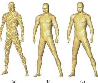
Figure 9 shows theMANmesh model evolving over 1,000 iterations of NODT

optimization (the mesh is chosen intentionally coarse and uniform for better vi-sual depiction). The figure depicts how going from 100 to 1,000 iterations brings further improvements on the mesh quality (confirmed by improvements over dis-tribution of dihedral angles and over number of remaining slivers). In meshes with variable sizing the improvement typically translates into 15% less leftover slivers. These experiments explain our will at accelerating every single optimization step.

Experiments in 3D show a good convergence of the average standard annulus width and average tolerance of vertices for the NODT mesh optimization process. However, the average tolerance of vertices converges in 3D to a proportionally

smaller value than the average standard annulus width compared with the 2D case (see Figures 6a and 10a). This is an effect of increasing the dimension and can be explained as follows: the average number of bi-cells including a given vertex is larger than 60 in three-dimensions (compare with the two dimensional case, which is 12). As explained in Section 2.3, the tolerance of a vertex z is half the min-imum of the standard annulus width of its adjacent bi-cells. In other words, the tolerance of a vertex is proportional to the minimum value of around 60 distinct standard annulus widths. Figure 10b quantizes how the standard deviation of the standard annulus widths in three-dimensions is larger than in two-dimensions. Fig-ures 11a and 11b show respectively the percentage of failFig-ures and the amount of tolerance updates per failure in two- and three-dimensions.

The rebuilding algorithm is considerably harder to outperform in three-dimensions for two main reasons. First, the removal operation is dramatically slower and the number of bi-cells containing a given point is five times larger than in two-dimensions. Nevertheless the filtering algorithm outperforms rebuilding for most input data considered in our experiments. In both two- and three-dimensions, it accelerates when going further on the number of iterations (see Figure 4.2). In three-dimensions, the main difficulty of this approach lies into the persistent quasi-degenerate cases. As the name suggests such cases consist of almost co-spherical configurations of the vertices of a bi-cell which persist across several iterations. The persistence mostly happens because the magnitude of the relocation moves decreases over time. Such cases lead to several consecutive filter failures, which themselves trigger expensive point relocations. In practice however, the amount of such degenerate configurations is rather small (see Figure 11c and Figure 11d).

Lastly we implement a small variation of the tolerance algorithm suggested in Section 3.2. The latter consists of rebuilding for the first few iterations before switching to the filtering algorithm. The switching criterion is more or less heuris-tic. Experimentally, we found that generally when 75% of the vertices remain inside their tolerance (55% in three dimensions), the performance of the filtering algorithm is more or less the same as rebuilding. This percentage can be used as a switching criterion. In our implementation we sample 40 random vertices at each group of four iterations and compute their tolerance. We compare these tolerances with their displacement sizes, and check if at least 75% of those vertices have their tolerance larger than their displacement size. In the positive we switch from the re-building to the filtering the algorithms. With this variant of the filtering algorithm, which is not dynamic for the first few iterations, we obtain an improvement in the running time of, e.g., 10% in the mesh optimization process of theHEARTmodel.

Mesh optimization schemes such as NODT [TWAD09] are very labor-intensive due to the cost of computing the new point locations and of moving the vertices. However, as illustrated by Figure 9, a large number of iterations provides us with

higher quality meshes. When optimization is combined with refinement, perform-ing more iterations requires not only reducperform-ing computation time of each iteration, but also additional experimental criteria. One example is the lock procedure which consists of relocating only a fraction of the mesh vertices [TWAD09]. In this ap-proach, the locked vertices are the ones which are incident to only high quality tetrahedra (in terms of dihedral angles). Each time a vertex move or a Steiner vertex is inserted into the mesh so as to satisfy user-defined criteria by Delaunay Refine-ment (sizing, boundary approximation error, eleRefine-ment quality), all impacted vertices are unlocked. Our experiments show that more and more vertices get locked as the refinement and optimization procedures go along, until 95% of them are locked. In this context the dynamic approach is mandatory as the mesh refinement and opti-mization procedure may be applied very locally where the user-defined criteria are not yet satisfied. Note also that the status of each vertex evolves along the itera-tions as it can be unlocked by the relocation of its neighbors. A static approach would slow down the convergence of the optimization scheme. In this context ac-celerating the dynamic relocations makes it possible to go further on the number of iterations without slowing down the overall convergence process, so as to produce higher quality meshes.

5

Conclusion

This paper deals with the problem of updating Delaunay triangulations for moving points. We introduce the concepts of tolerance and safe region of a vertex, and put them at work in a dynamic filtering algorithm which avoids unnecessary insert and remove operations when relocating the vertices.

We conduct several experiments to showcase the behavior of the algorithm for a variety of data sets. These experiments show that the algorithm is particularly relevant when the magnitude of the displacement keeps decreasing while the tol-erances keep increasing. Such configurations translate into convergent schemes such as the Lloyd iteration. For the latter, and in two-dimensions, the algorithm presented performs up to six times faster than rebuilding.

In three-dimensions, and although rebuilding the whole triangulation at each time stamp can be faster than our algorithm when all vertices move, our solution is fully dynamic and outperforms previous dynamic solutions. Such a dynamic prop-erty is required for practical variational mesh generation and optimization tech-niques. This result makes it possible to go further on the number of iterations so as to produce higher quality meshes.

Acknowledgments The authors wish to thank the anonymous referees for their insightful comments and Hans Lamecker for the HEART model. This work has

been supported by the ANR Triangles, contract number ANR-07-BLAN-0319, and Région PACA.

References

[ABE97] AMENTAN., BERNM., EPPSTEIND.: Optimal point placement for

mesh smoothing. In Symp. on Discrete Algorithms (1997), 528–537. [ABTT08] ACARU. A., BLELLOCH G. E., TANGWONGSAN K., TÜRKO ˘GLU

D.: Robust kinetic convex hulls in 3D. In European Symp. on Algo-rithms(2008), 29–40.

[ACD∗_{03] A}

LLIEZ P., COLIN DE VERDIÈRE E., DEVILLERS O., ISENBURG

M.: Isotropic Surface Remeshing. In Shape Modeling International (2003), 49–58.

[ACYD05] ALLIEZP., COHEN-STEINERD., YVINECM., DESBRUNM.:

Vari-ational Tetrahedral Meshing. ACM Transactions on Graphics 24 (2005), 617–625.

[AGMR98] ALBERSG., GUIBASL. J., MITCHELLJ. S. B., ROOST.: Voronoi

diagrams of moving points. Int. J. of Computational Geometry and Applications 8(1998), 365–380.

[Aur91] AURENHAMMER F.: Voronoi diagrams: A survey of a fundamental

geometric data structure. ACM Computing Surveys 23, 3 (1991), 345– 405.

[AV07] ARTHUR D., VASSILVITSKII S.: K-means++: The advantages of

careful seeding. In Symp. on Discrete Algorithms (2007), 1027–1035. [BDP∗_{02] B}

OISSONNAT J.-D., DEVILLERS O., PION S., TEILLAUD M.,

YVINEC M.: Triangulations in CGAL. Computational Geometry:

Theory and Applications 22(2002), 5–19. [BFG∗_{08] B}

RÖNNIMANN H., FABRI A., GIEZEMAN G.-J., HERT S., HOFF -MANNM., KETTNERL., SCHIRRAS., PIONS.: 2D and 3D

geome-try kernel. In CGAL User and Reference Manual, Board C. E., (Ed.), 3.4 ed. 2008.

[CDE∗_{99] CHENG S.-W., DEY T. K., EDELSBRUNNER H., FACELLO M. A.,}

TENGS.-H.: Sliver exudation. In Symp. on Comp. Geometry (1999),

1–13.

[CG06] CAZALS F., GIESENJ.: Delaunay triangulation based surface

recon-struction. In Effective Computational Geometry for Curves and Sur-faces, Boissonnat J.-D., Teillaud M., (Eds.). Springer-Verlag, Mathe-matics and Visualization, 2006.

[Che04] CHENL.: Mesh smoothing schemes based on optimal Delaunay

tri-angulations. In International Meshing Roundtable (2004), 109–120. [DBC07] DEBARD J.-B., BALP R., CHAINER.: Dynamic Delaunay

tetrahe-dralisation of a deforming surface. The Visual Computer (2007), 12 pp.

[DE06a] DU Q., EMELIANENKO M.: Acceleration schemes for computing

centroidal Voronoi tessellations. Numerical Linear Algebra with Ap-plications 13(2006).

[DE06b] DU Q., EMELIANENKO M.: Recent progress in robust and quality

Delaunay mesh generation. J. of Computational and Applied Mathe-matics 195, 1 (2006), 8–23.

[DEJ06] DU Q., EMELIANENKO M., JU L.: Convergence of the Lloyd

al-gorithm for computing centroidal Voronoi tessellations. SIAM J. on Numerical Analysis 44, 1 (2006), 102–119.

[Dev02] DEVILLERS O.: The Delaunay hierarchy. Int. J. Found. Comput. Sci.

13(2002), 163–180.

[DLM04] DEVROYEL., LEMAIREC., MOREAUJ.-M.: Expected time analysis

for Delaunay point location. Computational Geometry: Theory and Applications 29(2004), 61–89.

[DLPT98] DEVILLERS O., LIOTTA G., PREPARATA F. P., TAMASSIA R.:

Checking the convexity of polytopes and the planarity of subdivisions. Computational Geometry: Theory and Applications 11(1998), 187– 208.

[Ede01] EDELSBRUNNER E.: Geometry and Topology for Mesh Generation.

[For87] FORTUNES. J.: A sweepline algorithm for Voronoi diagrams. Algo-rithmica 2(1987), 153–174.

[FT06] FOGELE., TEILLAUD M.: Generic programming and the CGAL

li-brary. In Effective Computational Geometry for Curves and Surfaces, Boissonnat J.-D., Teillaud M., (Eds.). Springer-Verlag, Mathematics and Visualization, 2006.

[GLR97] GARCIA-LOPEZJ., RAMOSP. A.: Fitting a set of points by a circle.

In Symp. Comp. Geometry (1997), 139–146.

[GR04] GUIBAS L., RUSSEL D.: An empirical comparison of techniques

for updating Delaunay triangulations. In Symp. on Comp. Geometry (2004), 170–179.

[GS78] GREEN P., SIBSON R.: Computing Dirichlet tessellations in the plane. The Computer J 21, 2 (1978), 168–173.

[Gui98] GUIBAS L. J.: Kinetic data structures: a state of the art report. In

Workshop on the Algorithmic Foundations of Robotics(1998), 191– 209.

[HW79] HARTIGAN J. A., WONG M. A.: Algorithm AS 136: A k-means

clustering algorithm. Applied Statistics 28, 1 (1979), 100–108. [Llo82] LLOYD S.: Least squares quantization in pcm. Information Theory,

IEEE Transactions on 28, 2 (1982), 129–137. [LWL∗_{08] L}

IU Y., WANG W., LÉVY B., SUN F., YAND.-M., LU L., YANG

C.: On Centroidal Voronoi Tessellation—Energy Smoothness and Fast Computation. Tech. Rep. TR-2008-18, Dept. of Computer Sci-ence, Univ. of Hong Kong, 2008.

[ORSS06] OSTROVSKYR., RABANIY., SCHULMANL. J., SWAMYC.: The

ef-fectiveness of Lloyd-type methods for the k-means problem. In Symp. FOCS(2006), 165–176.

[PS90] PREPARATA F. P., SHAMOS M. I.: Computational Geometry: An

Introduction, 3rd ed. Springer-Verlag, Oct. 1990.

[PT08] PION S., TEILLAUD M.: 3D triangulations. In CGAL User and

Reference Manual, Board C. E., (Ed.), 3.4 ed. 2008.

[Rus07] RUSSELD.: Kinetic Data Structures in Practice. PhD thesis, Stanford

[SG86] SABINM. J., GRAY R. M.: Global convergence and empirical con-sistency of the generalized Lloyd algorithm. IEEE Transactions on Information Theory 32, 2 (1986), 148–155.

[SH75] SHAMOS M. I., HOEY D.: Closest-point problems. Symp. FOCS

(1975), 151–162.

[She96] SHEWCHUKJ. R.: Triangle: Engineering a 2D quality mesh

gener-ator and Delaunay triangulgener-ator. In Applied Computational Geometry: Towards Geometric Engineering, vol. 1148. Springer-Verlag, 1996, 203–222.

[She05] SHEWCHUKR.: Star splaying: an algorithm for repairing Delaunay

triangulations and convex hulls. In Symp. on Comp. Geometry (2005), 237–246.

[TAD07] TOURNOISJ., ALLIEZP., DEVILLERSO.: Interleaving Delaunay

re-finement and optimization for 2D triangle mesh generation. In Mesh-ing Roundtable Proc.(2007), 83–101.

[TWAD09] TOURNOIS J., WORMSERC., ALLIEZP., DESBRUN M.:

Interleav-ing Delaunay refinement and optimization for practical isotropic tetra-hedron mesh generation. ACM/SIGGRAPH Transactions on Graphics 28(3)(2009).

[VCP08] VALETTES., CHASSERYJ. M., PROSTR.: Generic remeshing of 3D

triangular meshes with metric-dependent discrete Voronoi diagrams. IEEE Transactions on Visualization and Computer Graphics 14, 2 (2008), 369–381.

[Yvi08] YVINEC M.: 2D triangulations. In CGAL User and Reference

(a) (b) (c)

Figure 9: Mesh quality improvement. (a)MANinitially; (b), (c)MANafter 100

and 1,000 iterations respectively.

0 200 400 600 800 1000 iteration 0 0.1 0.2 0.3 0.4 0.5 si ze average tolerance average annuli width

d isp la ce me n t (a) evolution 0 0.2 0.4 0.6 0.8 1 size Iteration 1000 Iteration 100 Iteration 10 Ite ra tio n 1 (b) distribution

Figure 10: Statistics in 3D. Consider a sphere such that the quantity representing the number of points divided by its volume is equal to 1. The cubic root of this quantity is the unity of distance. The figures depict 1,000 iterations of the mesh-ing optimization process onSPHERE: (a) evolution of the average displacement

size, average standard annulus width and average tolerance of vertices over 1,000 iterations; (b) distribution of the standard annulus width for 1, 10, 100 and 1,000 iterations.

0 200 400 600 800 1000 iteration 0 0.2 0.4 0.6 0.8 1 fa il u re s BUNNY LLOYD 2D (a) 0 200 400 600 800 1000 iteration 0 20 40 60 80 u p d a te s BUNNY LLOYD 2D (b) 0 200 400 600 800 1000 iteration 0 0.2 0.4 0.6 0.8 1 fa il u re s BUNNY SPHERE (c) 0 200 400 600 800 1000 iteration 40 50 60 70 80 u p d a te s BUNNY SPHERE (d)

Figure 11: Filter failures and number of tolerance updates. Consider the ex-ecution of the filtering algorithm for: the two-dimensional data set of Lloyd’s iterations with ρ = x2_{; BUNNY and SPHERE. The curves depict the percentage}

of relocations for which the filter fails along the iterations, for (a)BUNNY and

Lloyd’s iteration with ρ = x2_{, (c) BUNNY and SPHERE; the average number of}

tolerance updates done per filter failure, for (b)BUNNYand Lloyd’s iteration with

ρ = x2, (d)BUNNY andSPHERE. Observe how the complexity is higher for the

three-dimensional cases. Also note how the number of filter failures is higher for

BUNNYcompared toSPHERE(around 25% forBUNNYagainst 16% forSPHERE

0 200 400 600 800 1000

iteration

sp

e

e

d

u

p

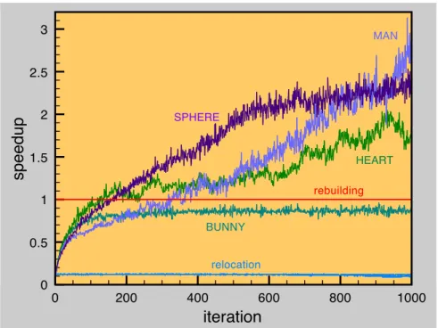
Figure 12: Speedup factors: NODT. The figure represents the speedup factor of each algorithm with respect to the rebuilding algorithm along the iterations, for a given input. Names with capital letters (e.g. “SPHERE”) in the figure, means

the filtering algorithm working in the respective input data (e.g. SPHERE). The

“speedup” of the relocation algorithm with respect to rebuilding is more or less constant for each input data.