The coupled nonlinear dynamics of spacecraft with fluids in tanks of arbitrary geometry

(1)

The Coupled Nonlinear Dynamics of

Spacecraft with Fluids in Tanks of Arbitrary

Geometry

MARTHINUS CORNELIUS VAN SCHOOR Mech. Eng, Pretoria University, (1982) SM, Massachusetts Institute of Technology, (1985)

SUBMITTED TO THE DEPARTMENT OF AERONAUTICS AND ASTRONAUTICS IN PARTIAL FULFILLMENT OF THE REQUIREMENTS

FOR THE DEGREE OF DOCTOR OF PHILOSOPHY

at the

MASSACHUSETTS INSTITUTE OF TECHNOLOGY

March, 1989

© Massachusetts Institute of Technology, 1989

kA..?.

Signature of Author ___.._

Department of Aeronautics and Astronautics

- March 24, 1989 Certified by Certified by Certified by Certified by Accepted by •a,•.mw- --- -,-, - - - - -•--- - - -•-m.. ---.

--Prof. Edward F. Cra'C;;iC mittee _airman

--- ' --- ". v -Z

Prof. Triantaphyllos R. Akyla, esis Committee (Department of Mechanical Engineering)

-Prof. JohnDugundji, Thesis Committee

Profr R&4hn Hansmanj Thesis Committee

• ~;•-•rof. Harold Y. Wachman i iairman, epartment Graiu' ate Committee

OFTASSHUS BT INST Y . OF TECHN4OLOGY _ _ JUN 07 1989 UrnmAW5$ WqITHDRWNi

M.I.T,

(2)

The Coupled Nonlinear Dynamics of Spacecraft with Fluids

in Tanks of Arbitrary Geometry

by

Marthinus C. van Schoor

Submitted to the Department of Aeronautics and Astronautics on March 30th, 1989 in partial fulfillment of the requirements for the Degree of

Doctor of Philosophy. Abstract

The nonlinear dynamics of a spacecraft coupled to a contained fluid with a free surface is studied both experimentally and analytically. A general finite degree-of-freedom, nonplanar model describing the dynamics of a spacecraft coupled to a fluid, contained in a tank of general geometry, is developed and verified by comparing analytical with experimental results.

The nonlinear model of the fluid/spacecraft system is accurate to third order in terms of the fluid motion amplitudes. A generalized coordinate description is obtained by satisfying the free surface boundary condition in an assumed mode approach. The kinematic boundary problem, posed as a variational problem, provides the relationship between the assumed free surface generalized coordinates and the fluid flow potential coordinates. Given the generalized coordinate description of the fluid, linear and nonlinear capillary forces, along with the standard energy terms, are included in the fluid Lagrangian. This method is valid for tanks with straight and parallel walls but results are presented which show that the method can be applied to tanks of more complex geometry if the geometry can be approximated with a straight/parallel wall assumption. In this research, the linear eigen-mode shapes as calculated with a finite difference routine, are used as assumed modes.

The nonlinear set of equations obtained by applying Lagrange's principle to the fluid Lagrangian, is solved for the forced response characteristics by numerical implementation of the Harmonic Balance method. The nonlinear time independent equations provided by this method are solved using an Inverse Iteration technique as well as a Newton-Raphson solver. The analytical model is used to investigate the nonlinear fluid slosh behavior in spherical, square, rectangular and cylindrical tanks.

Three scaled fluid tank models, namely; spherical, square and rectangular, were experimentally tested to determine the nonlinear characteristics of fluids contained in these types of tanks. The tanks are scaled to have Bond numbers representative of typical spacecraft fluid storage tanks. Both uncoupled (tank alone) and coupled forced excitation

(3)

tests are performed. In the coupled tests, the measured reaction slosh force is fed to an analog simulation of a spacecraft's modal dynamics, thus coupling spacecraft and fluid slosh dynamics. In these tests, the effects of system mass ratio, frequency ratio and damping ratio on the nonlinear coupled behavior are investigated.

The analytical and experimental results contributed to a general understanding of the complex behavior of fluid/spacecraft dynamic systems. In conclusion, tank vibrations exceeding 5% of the equivalent diameter show significant nonlinear effects, both in the fluid and spacecraft responses. The equivalent diameter is equal to four times the surface area divided by the circumference. For cylindrical tanks the equivalent diameter is equal to the tank diameter. At higher excitation levels (resonance amplitudes greater than 10-15% of the equivalent diameter), all the tanks exhibit jump phenomena and multi-valued oscillations. Convective (kinematic) fluid nonlinearities are important for all Bond numbers and capillary effects must be modeled for Bond numbers as high as 60.

Nonlinearities are the strongest for systems with low fluid mass fractions and for fluid-to-spacecraft frequency ratios between 0.8 and 1.0.

The experimentally observed amplitude dependent dissipation rates and shift in resonant frequencies (softening) are predicted by the analytical model. The model fails to predict the forced response characteristics when swirling motion occurs in the tanks which have repeated eigen-modes. If perturbed, to include a small coupling term between the spacecraft degree-of-freedom and the nonplanar slosh mode, the analytical model can predict the swirling motion. However a more detailed model of the nonplanar degree-of-freedom of the excitation system is required to correctly model the forced response characteristics when swirling occurs.

Thesis Supervisor: Prof. Edward F. Crawley

(4)

Acknowledgements

I dedicate this thesis to my caring and loving wife, Marcelle and to my parents. Marcelle not only sacrificed her own studies to enable me to come to M.I.T. but she also constantly supported and encouraged me and made a major contribution to this document. My parents love and faith in me carried me through the difficult times.

I would like to express my appreciation and thanks to my advisor, Prof. Edward Crawley, for his guidance, insight and support over the last two years. Without him this would not have been possible. The contributions of my thesis committee, Prof. T. Akylas, Prof. John Dugundji and Prof. John Hansman are also appreciated. It was a privilege to have you on my committee. A special word of thanks to Prof. Andy von Flotow. He was always available to discuss new ideas or to suggest a new direction.

The support and friendship of so many people made our time at M.I.T. a great, fulfilling experience. The people in my laboratory always had time to help me and to join us on Friday evenings. A special word of thanks to two very special people; Javier and Dave. You two, along with Mindy and Jean, mean so much to us. I hope we will be friends for ever.

The rugby crowd, especially Leo Casey, Mike Murphy, Bruce Johnson, Jim Culliton and Joan Rice must also be mentioned. Hanging around them prevented me from becoming a complete workaholic. May there be many more tries and victory celebrations.

This research was supported by NASA Headquarters Grant NAGW-21, with Mr. Samuel Venneri as technical monitor. The support of NASA is greatly acknowledge.

Vrystaaaat !!!!!

(5)

4.2.1 Slosh Force Reaction Balance and Resolver ... 4.2.2 Dry Mass Compensator ... 4.2.3 Signal Conditioning ... 4.2.4 Measuring the Tank Motion ... 4.2.5 Compliant Actuator ... 4.2.6 Data Acquisition and Experimental Control ... Test Procedures ... 4.3.1 Pre-Test Procedure ... 4.3.2 Test Procedure ... ...

4.3.3 Post-Test Procedure ... Calibration ... ... 4.4.1 Calibration of the Compliant Actuator ... 4.4.2 Proximeter Calibration ... 4.4.3 Calibration of the Force Resolver ...

Signal Conditioning Electronics

4.4.4 Calibration of the Planar Slosh ... Force Measurement

4.4.5 Summary of the Calibration Results ... Summary ... Experimental Results ... ...

Non-dimensionalization and Data Presentation ...

5.1.1 Uncoupled Tests ... ...

5.1.2 Coupled Tests ... ...

Spherical Tank Model ... ...

5.2.1 Spherical Tank Test Matrix ...

5.2.2 Spherical Tank Experimental Results ...

5.2.2.1 Discussion of the Uncoupled Test Results

5.2.2.2 Discussion of the Coupled ... Test Results

Square Tank Model ... ... 5.3.1 Square Tank Test Matrix ...

104 107 109 110 111 113 114 119 119 120 122 123 123 125 126 127 128 128 129 129 129 132 135 137 139 139 140 164 166

(8)

5.4 5.4 5.5 Chapter 6: 6.1 6.2 6.3 6.4

5.3.2 Square Tank Experimental Results ... 5.3.2.1 Discussion of the Uncoupled ...

Test Results

5.3.2.2 Discussion of the Coupled ... Test Results

Rectangular Tank Model ... ...

5.4.1 Rectangular Tank Test Matrix ... 5.4.2 Rectangular Tank Experimental Results ...

5.4.2.1 Discussion of the Uncoupled ... Test Results

5.4.2.2 Discussion of the Coupled ... Test Results

Cylindrical Tank Model ... ...

Sum m ary ... Analytical Results ... Analytical Modeling Issues ... 6.1.1 Equilibrium Free Surface ... 6.1.2 Calculation of the Linear Eigen-Mode ...

Shapes

6.1.3 Contact Angle Hysteresis Effects ... 6.1.4 Analytical Models ...

6.1.4.1 Assumed Mode Shape Selection ... 6.1.4.2 Fluid Dissipation Effects ... Forced Response Characteristics ... 6.2.1 Implementation Issues ... 6.2.2 Modeling Issues ... ...

6.2.3 Summary ...

Comparison of Analytical and ... ... Experimental Results

6.3.1 Cylindrical Model Tanks ... 6.3.2 Spherical Model Tank ... 6.3.3 Square Model Tank ... 6.3.4 Rectangular Model Tank ... Summary ... 168 168 169 196 197 200 200 202 228 231 232 233 233 237 243 244 244 258 258 259 266 277 277 277 283 289 295 305

(9)

Chapter 7:

7.1 7.2 7.3

Conclusions and Recommendations ... Sum m ary ... ... Conclusions ... Recommendations ... ...

R eferences ... ...

Appendices

Appendix A: Nonlinear Fluid/Spacecraft Equations ... of Motion

A1.0 Nonlinear Equations of Motion ...

A2.0 Model Truncation and Simplification ...

A3.0 Non-dimensionalization ... A4.0 Summary ... Appendix B: Planar and Nonplanar Models ...

B1.0 Planar Model ... B2.0 Nonplanar Model ... ... 306 306 307 310 312 318 318 321 324 327 328 329 332

(10)

Nomenclature

a Tank radius

(al,a2,a3) Accelerations measured by the accelerometers mounted on the test model base

ax Planar tank acceleration component ay Nonplanar tank acceleration component

amn Nonlinear equivalent fluid slosh depth matrix a(O) _{Zero'th order equivalent fluid slosh depth matrix}

(1)

amn _{Linear correction to the nonlinear equivalent fluid slosh depth} matrix

(2)

amn _{Quadratic correction to the nonlinear equivalent fluid slosh} depth matrix

Bo Bond number

c Damping constant for the spacecraft mode

Cqi Damping constant for the ith fluid mode Surface Area de Equivalent diameter = 4 Surface C ren

Surface Circumference

d mn Nonlinear kinematic matrix

(0)

mn _{Zero'th order kinematic matrix}

(1)

mn _{Linear correction to the nonlinear kinematic matrix} (2)

dmn _{Quadratic correction to the nonlinear kinematic matrix}

d Tank diameter

f Free surface equilibrium position, dimensional

(F1,F2,F3) Forces measured by the force reaction balance force transducers

(11)

fo, fo Spacecraft mode natural frequency

fs Primary planar fluid mode natural frequency Fxs Planar (x) reaction slosh force component Fys Nonplanar (y) reaction slosh force component Fx Total planar force component measured Fy Total nonplanar force component measured g Apparent acceleration at a tank location go Earth normal gravity (9.81 m/s2)

G Linear system reactance matrix

GC Spacecraft mode feedback gain corresponding to damping ratio Go Spacecraft mode feedback gain corresponding to frequency

Gm Spacecraft mode feedback gain corresponding to mass

h Fluid depth

I Kinematic integral which is minimized to satisfy fluid boundary conditions

IzD Total moment of inertia of the dry mass of the model tank and mounting hardware

kmn Nonlinear fluid wave number matrix

(0)

mn _{Zero'th order fluid wave number matrix}

(1)

kmn _{Linear correction to the fluid wave number matrix} (2)

kmn _{Quadratic correction to the fluid wave number matrix} k Spacecraft mode spring rate

K Stiffness matrix

Ka Accelerometer sensitivity (mvolts/g) Kx Proximeter sensitivity (volts/inch)

(12)

Normal accelerometer sensitivity (volts/g) Equivalent mechanical slosh model spring rate Nonlinear fluid wavelength matrix

Kg

Kn

Imn (0) Imn (1) imn (2) Imn L m mD mF mp mr mxq, myq Mzs Mz N

Zero'th order fluid wavelength matrix

Linear correction to the fluid wavelength matrix Quadratic correction to the fluid wavelength matrix Lagrangian of the coupled fluid-spacecraft system Spacecraft modal mass

Total dry mass inertia of the model tank and mounting hardware

Total fluid mass

Proof mass used in the force measurement calibration

Residual null-out dry mass in the force measurement calibration

Fluid-spacecraft inertial coupling coefficients Vertical slosh reaction moment component

Total vertical reaction moment component measured

Number of modes in the assumed modal decomposition of the fluid dynamics

Gravity scaled viscosity

Surface tension scaled viscosity

Outward pointing normal to the fluid volume V on the surface SF (including free surface and container walls)

Free surface modal coordinates Radial coordinate, dimensional

Radial coordinate, units of tank radius Inertial coordinates of the tank frame origin N_V2

(13)

rT Radius of the force transducer center-lines on the slosh force reaction balance

ra Radius of the accelerometer center-lines on the slosh force reaction balance

rh Hydraulic radius

RC Time constant of the spacecraft mode circuit Rcg Spacecraft orbital radius at the center of gravity s Laplace's variable

SF Fluid free surface SB Tank cross section

t Time

TF Total fluid kinetic energy Ts/c Spacecraft mode kinetic energy

u Fluid potential velocity relative to coordinate system fixed in the tank

u,v Curvilinear coordinate system defining the boundary of an enclosed fluid

ul, u2 Amplitudes of the complex eigen-mode coefficients, A1 and A2

ux i., u q _{Linear system eigen-mode coordinates}

UG Free surface gravitational potential energy

Us/c Spacecraft mode potential energy

Ua Free surface capillary potential energy

Vfex Input voltage of the compliant actuator spacecraft mode circuit

Vfxs Planar slosh force measurement voltage

Vfys Nonplanar slosh force measurement voltage

Vx Proximeter displacement measurement voltage

Vxc Output voltage of the compliant actuator spacecraft mode circuit

(14)

x Planar tank displacement (coordinate)

xi Inertial velocity vector of a fluid particle y Nonplanar tank displacement (coordinate) z Vertical coordinate (parallel to gravity vector) zT Tank displacement from spacecraft center of gravity

Greek:

a Fluid-vapor-solid contact angle

ai, aijk Nonlinear convection (fluid modal inertia) coefficients

fi, Iijk Nonlinear capillary coefficients

Xn Fluid flow field potential mode shapes

V Gradient operator (2 or 3 dimensions, depending on the function)

E Small parameter (<<1)

Yijk Secondary fluid mode forced solution coefficients for the quadratic perturbation equation

F Linear hysteresis constant

11 Free surface height parallel to g vector x Linear fluid sloshing mass fraction

9 Coupled system mass ratio (total fluid over spacecraft mode)

4xq, Jyq Linear fluid-spacecraft inertial coupling coefficients i33' , 44 Secondary fluid mode mass ratios

v Coupled system frequency ratio (slosh over spring frequencies) V1, v2 Coupled system eigen-frequencies (units of spring-mass

(15)

V3, V4 Secondary fluid mode natural frequencies (units of spring-mass

frequency)

Q Excitation frequency

Fluid flow potential field

On Fluid flow potential field modal coordinates <f Fluid flow spatial modal coordinate

a Surface tension

os Slosh circular frequency ýn Free surface mode shapes

Zex Non-dimensional externally applied force

SSpacecraft mode damping ratio

ýqi Fluid mode damping ratio

Derivatives:

(') Total time derivative

(16)

Chapter 1 Introduction

This Chapter motivates the research on coupled spacecraft/fluid systems (Section 1.1), discusses the underlying assumptions on which the assumed mode analytical model is based (Section 1.2) and explain how this analytical model was modified in this research to be valid for tanks of more complex geometry (Section 1.3). The chapter concludes with an outline of this document.

1.1 Research Motivation

The precise operating requirements of modern spacecraft demand a detailed model of all the on board dynamic components. Nonlinearities that were ignored in the past, must be modeled and understood in order to satisfy stringent operating requirements. For example; the resolution of orbiting optical systems can be significantly degraded by imperfections of 10-5 radians. Furthermore, attitude errors during transfer orbit insertion can result in a fuel mass penalty for the spacecraft. Since unmodeled dynamics during the design phase can result in sub-standard system performance and lead to instabilities, the modeled spacecraft dynamics must reflect the design requirements. For very tight tolerances, this will invariably lead to a very complex model. Effects, that may have to be modeled are; nonlinear geometric and material properties and multi-body dynamic effects.

Another potentially important nonlinear effect is fluid slosh. Nonlinear fluid/spacecraft motion caused by finite amplitude fluid slosh will depart significantly from motion predicted by linear theory. Liquid propellants are more efficient than solid propellants and more spacecraft designs rely on liquid propellants than ever before. Communication satellites carry as much as 50% of their total mass as liquid, both for orbital transfer and for attitude control. Liquid-fueled upper stages and orbital transfer vehicles can have mass fractions as high as 120%. These large mass fractions, spacecraft dry mass versus propellant mass, indicate that the dynamics associated with the fuel slosh is of paramount importance. The

(17)

longitudinal vibrations, also known as the pogo phenomena, observed in rockets and launch vehicles (for example; Thor-Agena and Titan II) [Kana in Abramson, 1966] and the fluid induced roll oscillations encountered in the Saturn I rocket program [Abramson, 1966] emphasize the need to accurately model the fluid slosh dynamics. Since it may be impossible to completely avoid interactions between the spacecraft motion and the contained fluid, this research is an attempt to develop a rational approach to the modeling of the coupled dynamics associated with spacecraft carrying contained fluids.

In the past many researchers have published work on this topic, namely; Reynolds and Satterlee [1964, 1966], Luke [1967], Yeh [1967], Abramson [1963, 1966] and Ibrahim [1975a, 1975b] and in the recent past; Peterson [1987] on the coupled nonlinear dynamics of fluid/spacecraft systems with cylindrical tanks, Agrawal [1987] on the interaction between liquid propellant slosh modes and attitude control in a dual-spin spacecraft, Berry [1981] on modeling large amplitude propellant slosh, Kanan [1987] on modeling nonlinear rotary slosh in propellant tanks, Komatsu [1987] on the analysis of nonlinear sloshing of liquids in tanks with arbitrary geometries, Nakayama [1981] on using the boundary element method to analyze two-dimensional nonlinear sloshing problems and Yu [1987] on the nonlinear analysis of sloshing in circular cylindrical tanks using the perturbation method. This list, far from a complete one, illustrates the considerable importance the engineering community has attached to the nonlinear fluid slosh problem. Studying the literature on the subject, one can conclude that there are many innovative ways to approach and solve the problem. It is not clear, however, how to generalize most of these methods to tanks of arbitrary geometry while keeping the model simple. Some of the approaches yield unwieldy equations, require significant algebraic manipulation and are not computationally cost effective.

The Rayleigh-Ritz assumed mode approach, developed by Miles [1984a and 1984b] and modified by Peterson [1987] for low Bond numbers, was selected, in this research as a method that could best be extended to tanks of arbitrary geometry. The following section is devoted to the underlying assumptions and simplifications associated with the assumed mode approach, while the next section of this chapter explains how this method was modified for this research.

(18)

1.2 Assumed Mode Approach

This section discusses and outlines the assumed mode approach developed by Miles [1984a and 1984b] and Limarchenko [1978a, 1978b and 1980]. This method was modified by Peterson [1987] to be valid for low Bond numbers. The method starts out by assuming separate sets of generalized coordinates for the free surface motion and for the internal potential flow function. The kinematic boundary condition at the fluid free surface is then used to relate the fluid flow potential generalized coordinates to the free surface motion generalized coordinates. Given a unique, independent set of generalized coordinates, the fluid kinetic and potential energies are expressed in terms of the free surface generalized coordinates and combined to form the system Lagragian. The next few paragraphs outline the underlying assumptions of the assumed mode model and identifies the important parameters.

Sources of Nonlinearities: The relationship between the fluid flow

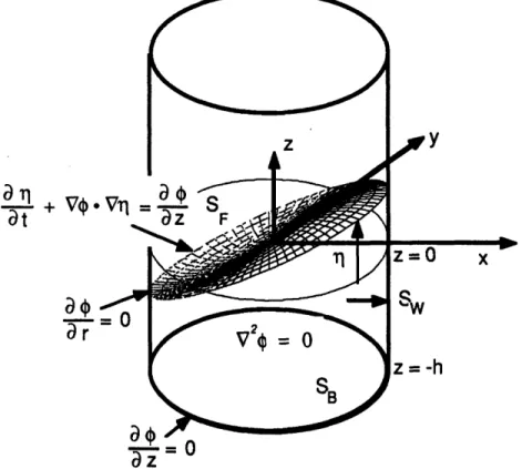
potential function generalized coordinates and the free surface generalized coordinates is nonlinear and is one of the major sources of nonlinearity in the fluid slosh behavior. Consider the action of the convection forces at the fluid free surface of the fluid. The potential flow (0) and the free surface motion (T1) must satisfy the kinematic boundary condition (Fig. 1.1):

at

+

I

z=

zz=T

(1.1)

This equation is an analytical expression of the Dirichlet and Neumann problems and constitutes a nonlinear relation between the fluid flow potential (0) and the free surface motion (01). Eq. 1.1 is a mathematical expression for the requirement that the fluid at the free surface boundary must follow the motion of the free surface.

Another source of nonlinearity is the potential energy stored in the capillary viscous forces [Limarchenko, 1981], given by:

U= of fV1+ VT V dS

s (1.2)

The potential energy of the free surface is a function of the total dynamic free surface area. The free surface area is a complex nonlinear function of

(19)

+ VO.

at

rr

Figure 1.1 Inviscid Fluid Flow Boundary Conditions for a Cylindrical Tank.

Fluid is constrained to flow parallel to the solid walls. The free surface boundary condition leads to nonlinear inertia effects in the fluid equations of motion.

the free surface shape (1i). Peterson [1987] extended the work of Miles [1984a] by expressing the free surface shape as a sum of the equilibrium or static free surface and the dynamic motion of the free surface. The capillary energy is then a function of the equilibrium free surface or Bond number (Bo). The Bond number is a non-dimensional measure of the relative importance of gravity versus capillary forces (eq. 1.3).

pga2

Bo-o (1.3)

In this equation (p) is the fluid density, (g) is the mean apparent gravity level, (a) is some fluid tank size scale factor and (a) is the surface tension.

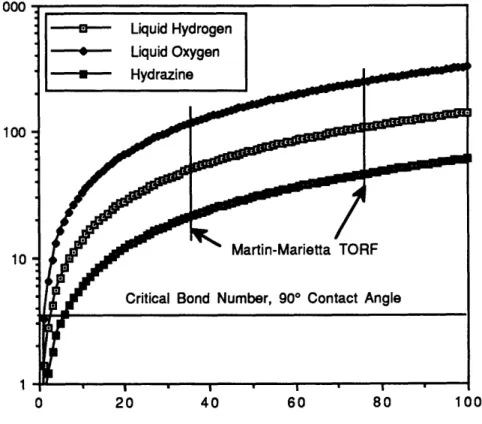
Fig. 1.2 depicts the Bond numbers for Hydrazine, Liquid Qxygen and Liquid Hydrogen due to gravity gradient, expressed as the tank displacement from the spacecraft's center of gravity, in a 3 m diameter cylindrical tank.

(20)

1000

100

10

1

0 20 40 60 80 100

Tank Displacement from Spacecraft CG (m)

Figure 1.2 Typical Bond numbers

In terms of the equilibrium free surface, gravity tends to minimize the free surface height and the capillary forces tend to minimize the free surface area. Many researchers [Satterlee and Reynolds, 1964; Myshkis, et al, 1987] have showed that at very low Bond numbers, the fluid can assume many stable configurations. Each equilibrium configuration of the fluid and vapor corresponds to a local minimum in the capillary-gravity potential energy expression. Large enough motions of the fluid container can re-orientate the fluid into another stable configuration. For Bond numbers above 200, gravity dominates and the fluid gathers in the bottom of the tank with a flat free surface. For moderate Bond numbers (below 100 and above a critical value), however, the capillary and gravity forces are comparable and the fluid has a curved free surface. Below a critical Bond number, the fluid equilibrium free surface is no longer stable and multiple configurations can exist. Each configuration is associated with a local minimum in the

(21)

capillary-gravity potential energy. A large enough perturbation of the tank will cause the fluid to re-orientate from one stable configuration to another. If the gravity vector reverses direction, there is critical Bond number at which the vibration frequency goes to zero. This corresponds to a static instability of the fluid, and is the critical re-orientation Bond number. The critical Bond number is a function of the contact angle (a) of the fluid at the tank wall and thus on the fluid type. For example, for a cylindrical tank the critical Bond number is given by:

Bo = -3.40 + 2.57 cos a

Critical _(1.4)

Low contact angle fluids are therefore less stable than high contact angle fluids. In this research however it is assumed that the Bond number is above the critical value (See Peterson [1987]) and that an equilibrium free surface exists.

Contact Angle Hysteresis Effects: Another effect that must be included

to correctly model the dynamics of the fluid, is the contact angle hysteresis effect. Satterlee and Reynolds [1964] showed that this effect can be linearized and included in the fluid description as an additional boundary condition at the fluid free surface contact contour with the container wall (eq. 1.5).

-n

_{-a ]}

_{on contact surface}

(1.5)

In this equation, T is the contact angle hysteresis constant which is a function of the fluid type and the tank wall surface and n is the normal to the tank wall at the free surface contact contour.

Fluid Flow Field Assumptions: The fluids considered in this

research as well as typical spacecraft propellants, can be considered as viscous and incompressible. Model simplifications can be justified based on the knowledge of the dominant physical behavior. Potential flow can be assumed if fluid viscous effects are restricted to the Stokes layer near the wall of the container. This condition is satisfied if the surface tension scaling parameter N,2 << _{1 (see eq. 1.7). In this research, given the model}

tanks and fluids used, N,2 ranges from 0.001 to 0.0014, justifying the potential flow assumption.

(22)

The viscous effects are included in the model as linear non-conservative damping forces. Predicting the fluid slosh damping can often only be done experimentally [Abramson, 1966], but analytical scaling analysis and estimation is possible [Miles, 1967]. For high Bond numbers, the fluid slosh damping scales with gravity and viscosity. The appropriate scaling parameter is:

NV

S• (1.6)

where (v) is the kinematic viscosity of the fluid. For low Bond numbers, eq. 1.6 must be multiplied with the Bond number (which is equivalent to scaling the Navier-Stokes equation using surface tension instead of gravity as the reference force), yielding an alternative scaling parameter:

N,= 2 (1.7)

These scaling parameters have been experimentally verified by Salzman and Masica [1969], who showed that the damping ratio at low Bond number is

approximately six times higher than the high Bond number value. Salzman and Masica suggested that this is due to the free surface curvature effects on the flow profile. Important to note is that baffles and propellant management devices can enhance the fluid damping. This, however, only produces a finite amount of damping and if the baffles are partially submerged, they tend to break up and separate the fluid oscillation modes which, incidentally, produces a very nonlinear geometric effect [Abramson,

196].

The analytical method of this research completely ignores all geometric nonlinear effects. Some of these effects are; partially submerged baffles that cause fluid flow impact, drainage and complex container walls that cannot be aligned with a curvilinear grid.

Container: The analytical model assumes a rigid container which

considerably simplifies the problem. This assumption is valid for containers that have structural frequencies spectrally separated from the dominant fluid slosh and control modes. The boundary condition at the tank walls, for a rigid tank, is simply that there is no flow normal to the tank wall. The previous paragraphs summarized the fluid flow assumptions and the rest of

(23)

this section will concentrate on the assumed coupled characteristics of the fluid/spacecraft system.

Recent studies of the coupled fluid/spacecraft problem have concluded that any proper model must be nonlinear in order to correctly model the coupling between the fluid and container motion. The problem of a water tower on flexible supports was analytically and experimentally studied by Ibrahim and Barr [1975a and 1975b] (Also see Ibrahim and Heinrich [1987]). Their analytical model did not include capillary effects, nor secondary fluid modal interactions. Peterson [1987], on the other hand, included these effects in his model to study a fluid/spacecraft configuration similar to the one considered in this research.

In order for the results to be applicable to a wide range of spacecraft, this research concentrated on coupled nonlinear dynamics of the system depicted in Fig. 1.3. In this figure, a fluid container (not necessarily a cylindrical container) is attached to a one degree-of-freedom spacecraft mode. The motion of the container, but not the fluid, is restricted to be in one direction (the x-direction or planar direction) only. The spacecraft degree-of-freedom can be either an attitude control mode or one of the support structure's modes. The stiffness, mass and damping of this mode may be tuned to study the coupling effects on the fluid/spacecraft dynamic behavior. The response of the coupled system will be dependent on the relative tuning between the primary fluid slosh mode and the spacecraft mode. The relevant non-dimensional parameters are therefore the mass ratio, the ratio of total fluid mass to total dry mass of the tank

mF

S- m _(1.8)

and the frequency ratio, the ratio between the fundamental fluid slosh frequency and the frequency of the spacecraft mode

fs

(24)

x(t)

F (0ex

Figure 1.3 Research Fluid/Spacecraft Study Model

One other non-dimensional parameter remains that will influence the fluid/spacecraft system response, namely the applied force:

F ex

"ex _{- k d}

(1.10)

where (k) is the stiffness of the spacecraft mode and (d) some scale length. Since the response will scale with =ex, given an absolute force level Fex, a more compliant (softer k) spacecraft will result in a more nonlinear response.

In practice, spacecraft have six degrees-of-freedom. Therefore the assumption that the nonplanar degree-of-freedom is infinitely stiff, that is;

(25)

vs/c in eq. 1.11 is assumed to be infinite, is only valid for the experimental setup of this research. Incidentally, it was found that this assumption was one of the major limitations of the analytical model used in this research.

s /c _(1.11)

1.3 Research Approach and Outline

This section outlines how the analytical method of Miles [1984a and 1984b] and Peterson [1987] was modified to be valid for tanks of arbitrary geometry, and describes the solution procedure used to determine the nonlinear characteristics of the fluid/spacecraft system along with the experimental studies that were performed to validate the analytical model.

In order to apply the assumed mode model developed by Peterson, the Taylor series expansion of the kinematic integrals [Peterson, 1987] had to be modified to be valid for a numerical grid curvilinear system. The method also had to be adapted for numerically derived eigen-modes. This allowed the nonlinear formulation to be valid for almost any tank geometry and also for tanks with baffles, as long as the baffles remain submerged during fluid oscillations. The method derived, however, is only valid for tanks with side-walls aligned with one of the curvilinear coordinates.

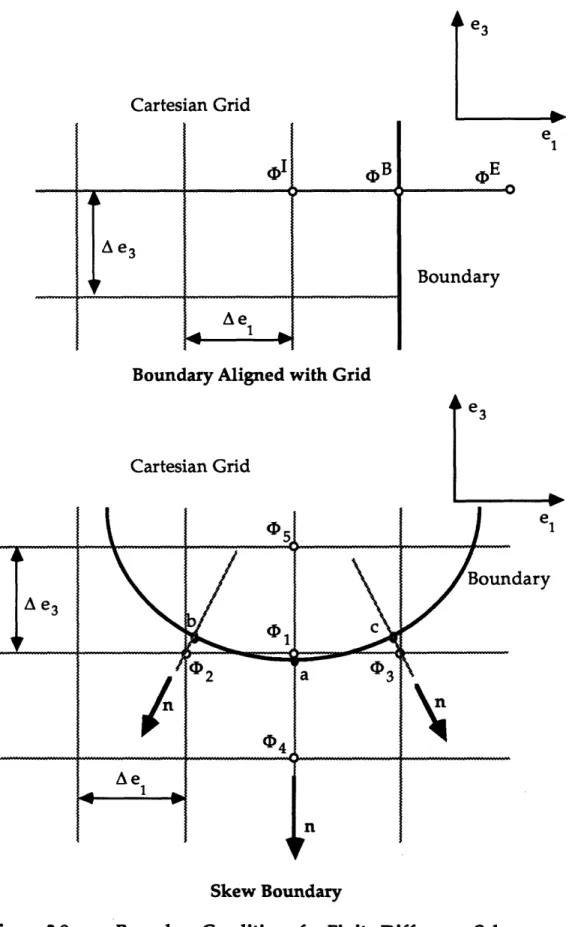
Although many standard computer packages exist on the market that can calculate the linear eigen-modes of the fluid in the container, a finite difference program was developed for flexibility, cost and data management reasons. The finite difference method used shape functions to implement the boundary conditions that are misaligned with the finite difference mesh. The effect of contact angle hysteresis was included to yield the experimentally observed linear eigen-frequencies.

In order to correctly model Bond number effects (the effect of the nonlinear capillary forces), the equilibrium free surface shape was calculated and added to the finite difference mesh of the linear eigen-routine. The capillary and acceleration potential energies were posed in a variational integral.

(26)

Test 410-1. Non-dimensional Tank Displacement (x/d). 0.1 0. x/d x101 0. 0. 0. 0.60 0.70 0.80 0.90 1.00 1.10 1.20 1.30 f/fo

Figure 1.4 An example of the Amplitude Dependent Dissipation Rates observed by Peterson [1987].

Euler's equation, which satisfies the requirement that the variational integral remains stationary with respect to independent variations, was used to solve for the Bond number-dependent equilibrium free surface. This was achieved by discretizing the free surface in a finite difference mesh and solving the resultant non-linear equations with an Inverse Iteration scheme. This approach is one of the major contributions of this research and it can be applied to tanks of arbitrary geometries.

Peterson [1987] used the Multiple-Time-Scales method to solve for the nonlinear forced response characteristics of the fluid/spacecraft system. This method can only predict the shift in resonant frequencies and failed to predict the amplitude dependent dissipation rates observed in the coupled system resonances (See Fig. 1.4). In this research, the Harmonic Balance Method is used to predict the coupled nonlinear forced response characteristics, using a full nonplanar model of the fluid/spacecraft system. The nonlinear time independent equations provided by this method are solved using both an Inverse Iteration Scheme and a Newton-Raphson solver with an adaptive under-relaxation scheme.

The objective of the experiments was to verify the analytical model and to extend the database on the dynamic behavior of coupled

(27)

fluid/spacecraft configurations. The experimental setup was essentially the same as the one used by Peterson. In this research, however, a personal computer was used to control the experiment, collect data and perform pre-data analysis. A spherical, square and rectangular tank were used as study models. The results obtained with these tanks, combined with the cylindrical tank results obtained by Peterson, were considered adequate to verify the analytical method.

1.4 Report Outline

Chapter 2 develops the nonplanar, nonlinear analytical model based on the assumed mode approach. The fluid flow potential generalized coordinates are related to the free surface generalized coordinates through the application of the kinematic free surface boundary conditions. The nonlinear relationship between these coordinates are formulated to facilitate the use of numerically determined eigen-modes. The finite difference method used to determine the linear eigen-modes is outlined as well as the determination of the equilibrium free surface shape. This chapter concludes with the fluid energy Lagragian.

Chapter 3 describes the Harmonic Balance method and how the method was numerically implemented. This chapter also discusses solution techniques other than the Harmonic Balance method and ways to solve systems of nonlinear equations.

Chapter 4 describes the experimental setup, and the test and calibration procedures. Chapter 5 presents the experimental uncoupled and coupled results obtained with the three study models.

Chapter 6 compares the analytical results obtained with the model developed in Chapter 2 with the experimental results of Chapter 5. In addition to the three study models, the analytical model was also used to predict the nonlinear coupled forced characteristics of fluids contained in cylindrical tanks. These results are compared with the results obtained by Peterson [1987].

Chapter 7 concludes with a short review of the research and conclusions that can be drawn from the experimental and analytical results.

(28)

This chapter also identifies the implications for future research and discusses the application of the results to practical systems.

Appendix A derives the nonplanar model from the system Lagragian obtained in Chapter 2. Appendix B presents simplified planar and nonplanar models based on the results of Appendix A. These models are simplified in the sense that zero terms are omitted and that the models are expressed in matrix form.

(29)

Chapter 2 General Nonlinear Fluid Model

This chapter develops and derives the equations of motion describing the nonlinear coupled dynamics of the fluid-spacecraft system. The analytical model developed is valid for tanks of arbitrary geometry.

The goal of the analytical formulation is a description of the fluid-spacecraft motion in terms of a finite set of system degrees of freedom. This description will be in the form of a coupled system Lagrangian and a set of coupled nonlinear differential equations derived from this Lagrangian.

The formulation of such a coupled system Lagrangian requires generalized coordinates for the motion of the spacecraft and the motion of the fluid. For the spacecraft in the study model, the generalized coordinates will be the physical displacement coordinates of the fluid tank in the horizontal plane (x and y). For the fluid, however, the choice of generalized coordinates is far more complicated.

The first part of this chapter will concentrate on the derivation of such a generalized coordinate description of the fluid motion. The kinematics (boundary conditions) are solved approximately with nonlinear and Bond number effects included. An expression for the kinetic and potential energy of the fluid system is formulated with nonlinear surface motion and nonlinear capillary effects included.

This chapter also outlines the approach that was used to calculate the linear fluid eigen-characteristics and the fluid free surface shape. In the final section, the generalized coordinate description of the fluid is used to formulate the coupled fluid-spacecraft Lagrangian.

2.1 Kinematic Description of the Fluid Dynamics

In this section, using existing methods, the kinematic description of the fluid is developed in terms of assumed modal series for the flow potential and the free surface motion. The flow potential generalized coordinates are expressed as nonlinear functions of the free surface

(30)

SPACECRAFT

Attitude Control Thrusters

g Apparent Gravity Field

Figure 2.1 General Fluid-Spacecraft System.

Fluid with a free surface is vibrating inside a spacecraft mounted fuel tank. Attitude control dynamics and structural modes may interact with fluid dynamics.

generalized coordinates through the application of a particular free surface boundary condition.

2.1.1 Problem Statement

Consider the general fluid-spacecraft system diagrammed in Fig. 2.1. A fluid tank, partially filled with a liquid, is supported by the spacecraft structure. The spacecraft motion is forced by attitude control thrusting, gravity gradient, or the action of any other external forces. When the mean gravity level produces a Bond number above the critical value, the fluid will collect into a single mass at the end of the tank aligned with the mean gravity vector, with a free surface at the other end. External excitation of the

(31)

Figure 2.2: Study Nonplanar Model.

The planar (x) direction is in line with the excitation force; the nonplanar (y) direction is perpendicular to the excitation force.

fluid tank will result in fluid vibratory response about this equilibrium shape.

The resultant vibratory response of the fluid inside the tank creates a fluid pressure field against the tank walls, which will have three dimensional force and moment fields. These reaction slosh loads will appear in the equations of motion for the dry dynamics of the spacecraft as motion-dependent forcing terms. In this manner, the fluid and the spacecraft motion are coupled.

(32)

Consider the generic fluid-spacecraft system (Fig. 2.2). The equation of motion for the spacecraft in the direction of excitation (planar direction) is

mi +cx + kx= Fex + Fxs _(2.1a)

and in the nonplanar direction:

my + c, + ky = F _YS (2.1b)_(2.1b)

Where x is the x-direction degree of freedom of the tank, y the y-direction degree of freedom, Fex the external modal load component evaluated at the tank, Fxs and Fys the net reaction slosh forces acting against the tank in the x and y directions.

The net reaction slosh force Fxs is the integration of the pressure field created by the fluid motion within the tank, and will therefore be a function of the fluid generalized coordinates, qn. The equations for these (as yet unspecified) fluid generalized coordinates can be symbolically expressed by a nonlinear equation:

N(q1,q1,... q2 , " _{.. /",112"..."}

2"i 2/ .. 91..) = N = 0 (2.2)

These equations, along with (2.1) form the coupled equations of motion of the fluid-spacecraft.

2.1.2 Modeling

Instead of evaluating and integrating the flow pressure field, which can be very complicated even for the simplest of tank geometries [Abramson, 1966], a variational energy method will be used which does not explicitly require the evaluation of the pressure field. This approach has been successfully used before [Peterson, 1987, Limarchenko, 1978a; 1981; 1983]. In the variational method, the virtual work done by the pressure field against the tank wall will be part of the total fluid kinetic energy, provided the flow boundary conditions have been satisfied by the choice of generalized coordinates.

The next step in modeling the fluid motion is to find a Lagrangian description of the fluid-spacecraft dynamics. Although the derivations for the spacecraft part of the Lagrangian are trivial, those of the fluid dynamics

(33)

are much more complicated. In particular, a generalized coordinate description of the fluid must be found which also satisfies the boundary conditions of the flow.

The modeling of the fluid-spacecraft dynamics can thus be separated into three distinct modeling steps.

* Model of the fluid motion consistent with the fluid boundary conditions (the Kinematic description of the fluid),

* Express the kinetic and potential energy of the fluid in terms of generalized coordinates, as derived in the first step, and

* Formulate the coupled system Lagrangian

Each of these steps will be discussed in the subsequent paragraphs.

2.1.3 Boundary Conditions

Some approaches in the past, such as Luke (1967), included the fluid boundary conditions as constraints in the Lagrangian. This will not be necessary if all the flow boundary conditions have been satisfied by the generalized coordinate flow fields. Choosing such generalized coordinates for the fluid is the 'kinematic problem' for the flow. Limarchenko (1978) solved this problem using the boundary condition differential equations in a Galerkin-type procedure. Miles (1976) provided a more general approach which uses a 'kinematic variational' to solve this problem. The approach used in this analysis is the approach used by Peterson, which is an adaptation of Miles's 'kinematic variational' method.

The main procedures and assumptions used in finding a generalized coordinate description of the fluid, are:

* Assume inviscid, incompressible flow.

* Postulate assumed modes for the free surface motion and the flow potential.

* Relate the flow potential generalized (modal) coordinates to the free surface generalized (modal) coordinates through a variational procedure.

(34)

Each of these procedures (and assumptions) will be discussed in the next sections.

2.1.3.1 Assumptions on the Fluid Flow Field and Boundary Conditions

In general, the fluid is a viscous, compressible continuum, and has a very complicated slosh behavior. Assumptions and simplifications, however, can be justified based on the knowledge of the dominant physical behavior.

Most of the following sections will assume a general curvilinear coordinate system (el, e2, e3). The actual coordinate system used for the four

study models considered in this research is:

* Cylindrical tanks Cylindrical Coordinate system (r, 0, z) Velocity Components: (ur, ue, uz)

* Spherical tanks Cartesian Coordinate System (x, y, z) Velocity Components: (ux, uy, uz) * Rectangular tanks Cartesian Coordinate System (x, y, z) (of which Square tanks Velocity Components: (ux, uy, uz) are a subset)

A cartesian coordinate system, instead of a spherical coordinate system, was used for the spherical model tanks since the equilibrium free surface is not aligned with one of the spherical coordinates. If the fluid viscous effects are restricted in a Stokes layer near the wall of the tank (N2 = v ₂ _a << 1), the fluid flow velocity u relative to the tank reference frame can be completely described by an irrotational, three dimensional potential field *. (See eq. 4.1b for a definition of the surface tension parameter N,2). In this research, given the model tanks and the modeling fluids used, the capillary viscous parameter (N, 2) range from 0.001 to 0.0014. :

(35)

Since the fluid is incompressible, the divergence of the velocity field must vanish throughout the fluid volume:

V*u = 0 (2.4)

The resulting partial differential equation describing the flow potential is the Laplace equation:

V20 = 0 _(2.5)

If 0 is continuous inside the fluid volume V, it will be completely and uniquely specified by its value and the value of its normal derivative

V4.n = (2.6)

at the boundary of the fluid (Hildebrand, 1976).

For the 'Dirichlet Problem', in which the value of 4 is prescribed at the fluid boundary, the solution to (2.5) will be unique in V. For the 'Neumann Problem', in which the value of ~p/an is prescribed at the fluid boundary, the solution to (2.5) will be unique within an additive constant in V. For the case of fluid flow in a closed container, only the velocity of the fluid at the boundary is specified, and so the fluid description is a Neumann Problem. Solution of Equation (2.5) will then lead to a unique value of VO in V, which will uniquely define the flow velocity field, u. What this means physically is that if the free surface motion is known, the fluid flow velocity profile will be completely specified.

Fig. 2.3 to 2.5 depicts the boundary conditions of the flow potential for the four study tanks considered in this research. For the cylindrical tank (Fig. 2.3) a cylindrical coordinate system (r, 0, z, t) is used. Three separate surfaces bound the fluid volume. The bottom of the cylinder is designated SB, the walls of the cylinder are designated Sw, and the free surface is designated SF. The free surface is defined by the surface il(r, 0, z, t) with 1 aligned with the z-axis. The following boundary conditions apply at each of these surfaces:

-0

0 z on SB _(2.7a) r 02a) r on Sw (2.8a)

(36)

-- + _V

_y

₌

Tt

71 z=1

= z Iz=1

on SF (2.9a)

The first two boundary conditions analytically state that the fluid does not penetrate the solid walls of the container. The third boundary condition, however, is a mathematical expression for the requirement that the fluid at the free surface (SF) must follow the motion of the free surface. This 'convective boundary condition' on the flow drives the dynamics of the fluid motion within the fluid volume V. It is also the principal source of the fluid slosh nonlinearity.

VO

0

"--" -- 0

atz

Figure 2.3 Inviscid Fluid Flow Boundary Conditions for a Cylindrical Tank. (Repeat of Figure 1.1)

(37)

Inviscid Fluid Flow Boundary Conditions for

Tank. a Spherical

For spherical, rectangular and square tanks it is convenient to use a

cartesian coordinate system. The free surface is defined by the surface

rl(x, y, z, t) with rl aligned with the velocity component uz. The boundary

conditions, for the spherical tank, (Fig. 2.4), are:

,r - 0

on Sw

+at VVlI az=

(2.7b)

on S_F (2.9b)

where Sw is the spherical surface of the tank.

r U

ar

(38)

--

+ Vo Vr-~ 7

O

Inviscid Fluid Flow Boundary

Rectangular and Square Tank.

Conditions

The boundary conditions for rectangular tanks (Fig. 2.5) (of which square tanks are a subset), are:

S-0 Sz -- =0 ax -0 ay on SB (2.7c) on SWx on SWy Figure 2.5 _{for a} (2.8c)

(39)

at +V tz=Iz a_ z z=1 on SF (2.9c) Sw, and Swy _{being the tank walls in the x- and y-directions respectively.}

2.1.4 Variational Solution of the Neumann Kinematic

Problem

While no general solution to the above nonlinear potential flow boundary value problem is known, approximate solutions can be found which are valid for finite motion of the free surface. The approach followed here assumes modal behavior for both the free surface and the flow potential. The generalized coordinates describing the flow potential are then related to the generalized coordinates describing the free surface motion using a variational expression for the Neumann problem.

Luke (1967) and Miles (1976) extended earlier work of Clebsch (1859) and Hargreaves (1908) to show that the general Neumann problem for fluid flow in containers can be satisfied by requiring that the integral of eq. 2.10 remains stationary with respect to arbitrary variations of the function *. Application of this integral to specific container geometries can be found in the literature, for example; Miles (1976) and Peterson (1987) - cylindrical tanks and Moiseev and Petrov (1966) - spherical tanks.

SI= JfJ(VOPVO)dV -

z,0

dS

2F

(2.10)

in which tl _{is the function describing the dynamic free surface, S the} equilibrium free surface area (as projected on the plane perpendicular to z-coordinate) and SF _{the dynamic free surface area. The requirement that the}

integral remains stationary for arbitrary fluid motion (84) yields Laplace's Equation (2.6) and the flow boundary conditions of eq.'s (2.7), (2.8), and (2.9).

This integral will be minimized by the exact nonlinear solution to the kinematic problem but in the absence of a known exact solution, an approximate solution to the kinematic problem can be found using assumed potential flow behavior and assumed free surface motion. The assumed motions are not independent and their relationship can be found by substituting the assumed motions into eq. 2.10 and requiring the result to be

(40)

stationary. This will result in a 'least squares' solution to the nonlinear boundary value problem. No mathematical preconditions are set on the assumed functions except that they be continuous in V.

This variational principle can be applied to any (single-valued) equilibrium free surface shape. In this research it will be applied to a moderate-to-low Bond number equilibrium curved free surface shape.

At this point it is assumed that the free surface and the fluid potential can be described by the superposition of finite modal sets. Ignoring geometric nonlinearities, that is assuming that the in-plane motion of the fluid can be neglected, the free surface motion Ti is described in terms of the departure from the equilibrium free surface shape f (Fig. 2.6) as:

N

rl(e ,e 2,t) = f(e ,e2) + 1 rn(e ,e2)qn(t)

n=l1

Ti(e 1,e2,t) = f(el,e2) + 2 d(e 1,e _29t)

(2.11)

(2.11a)

Equilibrium Free Surface

Dynamic Free

Coordinate System for Dynamic Free Surface and Equilibrium Free Surface Shape.

(41)

in which qn are the generalized coordinates for the free surface motion. Implied in eq. 2.11 is that iT is the coordinate defining the free surface shape.

In this research, 1l is the vertical coordinate (e3 or z) of the free surface height. For the cylindrical and rectangular tanks 11 completely describes the free surface, but for spherical tanks iT will define the free surface for

moderate amplitudes of free surface motion. Thus for a grid defined on the el-e2 plane f(el, e2) is the displacement, along the e3-axis, from the grid-plane

to the equilibrium free surface and Tld(el, e2, t) is the displacement, along the

e3-axis, of the dynamic free surface from the equilibrium free surface. In

order to obtain a correct definition of the free surface, a coordinate transformation will be required that will align surface motion with one of the axis. An arbitrary orthogonal coordinate system (e1, e2, e3) is used for

generality.

The fluid potential field O(el, e2, e3, t) is assumed to be of the form:

N

x(ele

2'e3t)= I Xm(el,e ₂,e3)P m(t)

m=1 (2.12)

in which the Pm are the generalized coordinates for the flow potential.

The number of modes describing the flow potential (M) and the free surface motion (N) are set equal to ensure that the problem is completely determined and that no additional least squares match is required. The number of modes N (N=M) to be used in the analysis will be kept arbitrarily large but will be truncated later to include only those which significantly

contributes to the fluid vibratory motion.

The two sets of generalized coordinates qn and Pm are related by the nonlinear free surface boundary condition (2.9), and are therefore not independent. Selecting the free surface generalized coordinates qn to be the independent fluid generalized coordinates, the flow potential coordinates (Pm) can be expressed as nonlinear functions of the free surface generalized coordinates qn.

Pm = _{P(q n)}

(42)

Substituting the assumed modal behavior into the kinematic integral of eq. 2.10, yields:

N N N N

SI= 1

1 mkmn•n-

4imdmnn

m=ln=l m=ln=1 (2.14)

in which the kinematic matrices are:

kmn

=

f(VXm'VXn)dV

V _(2.15)

dmn

=

f4mX

_{n z)dS}

SF

(2.16)

The matrix kmn is the generalized symmetric wavenumber matrix of the fluid motion, having units of inverse length The matrix dmn is both unsymmetrical and unitless. Both of these matrices are nonlinear functions of the free surface modal vector qn because the volume V depends on tl and the function Xn is evaluated on the free surface.

In matrix notation, (2.14) is the same as

SI= {pm}T[ kmn]{Pn } - {Pn}T [dmn]T'(m (2.17)

Now requiring that the kinematic integral remains stationary with respect to pij results in:

a(SI) =TPn1-d jT

-pj -ki]{Pn} -[dm]

= 0

0Am}

ap _(2.18)

by which the flow potential generalized coordinates Pm can be related to the free surface generalized coordinates qn by

NN -1

pm= XI [kmr] dnr4n

n=lr=l (2.19)

which is the same as

N

Pm= Imn2n (

(43)

1t~ TAThii9I fhn~ m~r I ic, Ct~t~ Ih, ILL VV L CLL LIL ; LCLLL A J• mn a •IUAL Uj

N -1

Imn I E[kmn] dnr

r=l (2.21)

The matrix Imn is the generalized nonlinear wavelength matrix, and is a nonlinear function of the modal vector qn. Equation (2.20) is the desired functional relation which expresses the potential generalized coordinates

(Pm) in terms of the free surface generalized coordinates (qn).

Based on the experimental results cubic and higher order terms in Imn of the generalized free surface coordinates will be considered as small. This truncation will yield a fluid flow description valid to cubic order in the amplitude of the motion.

2.1.5 Note on the Assumed Mode Shapes

The number and choice of the mode shape functions Xm and 4n will determine the ultimate accuracy of the above kinematic solution. Selection of these mode shapes must be based on experience, previous research or experimental results. In practice it may be required to progressively increase the number of assumed modes while keeping track of the relative change in the predicted fluid motion. Intuition also suggests that more accuracy will result from those assumed mode shapes that satisfy most of the kinematic conditions exactly. The linear eigen-modes of the slosh, which satisfy the linearized kinematic conditions, is an obvious choice, since the kinematic integral (I) would contain only error terms due to the nonlinear correction of the kinematic conditions. In Chapter 6 both theoretical mode shapes and numerically determined mode shapes are used to predict moderate-to-low Bond number fluid motion in cylindrical tanks. In predicting the fluid motion in spherical, rectangular and square tanks (Chapter 6) only numerically determined mode shapes were used.

An additional presumption is made about the two dimensional components of the assumed mode shapes. The assumed mode shapes must