Active combustion control : modeling, design and implementation

Active Combustion Control:

Modeling, Design and Implementation

by

Sungbae Park

M.S., Mechanical Engineering

Massachusetts Institute of Technology, 2001

Submitted to the Department of Mechanical Engineering

in Partial Fulfillment of the Requirements for the Degree of

Doctor of Philosophy

at the

Massachusetts Institute of Technology

June 2004

© 2004 Massachusetts Institute of Technology. All r

Signature of Author ... /.

...

LIBRARIES

ights reserved.

..

...

Department of Mechanical Engineering

May 7, 2004

... -...

Anuradha M. Annaswamy

Senior Research Scientist

Thesis Supervisor

Certified by ...

_...

Ahmed F. Ghoniem

Professor

Thesis Supervisor

Accepted by ...

Ain A. Sonin

Chairman, Department Committee on Graduate Students

Active Combustion Control:

Modeling, Design and Implementation

by

Sungbae Park

Submitted to the Department of Mechanical Engineering on May 7, 2004, in Partial Fulfillment of the

Requirements for the Degree of

Doctor of Philosophy in Mechanical Engineering

Abstract

Continuous combustion systems common in propulsion and power generation applications are susceptible to thermoacoustic instability, which occurs under lean burn conditions close to the flammability where most emissions and efficiency benefits are achieved, and near stoichiometry where often high power density can be realized. This instability is undesirable because the accompanying large pressure and heat release rate oscillations lead to high levels of acoustic noise and vibration as well as structural damage. Active control is one approach using which such instabilities can be mitigated. Over the past five to ten years, it has been shown conclusively through several lab-scale studies that active control is highly successful in suppressing the pressure oscillations. This success has set the stage for transition of the technology from laboratories to large-scale applications in propulsion and power generation. This thesis provides some of the building blocks for enabling this transition.

The first building block concerns the modeling of hydrodynamics and its interactions with the other components that contribute to combustion dynamics. The second is the impact of active control on emissions even while suppressing the pressure instability. The third is the evaluation of model-based active controllers in realistic combustors with configurations that include swirl, large convective delays and unknown changes in the operating conditions. The above three building blocks are investigated in the thesis experimentally in three different configurations. The first is a 2D backward facing step combustor, constructed at MIT, with the goal of investigating the flame-vortex interactions and the impact of active control on emissions. The second is a dump combustor, constructed at University of Maryland, so as to reproduce more realistic ramjet conditions. The third is an industrial swirl-stabilized combustor, constructed at University of Cambridge, to mimic realistic industrial gas combustor configurations which typically include large convective time delays, swirl, and on-line changes in the operating conditions. Results obtained from these three configurations show that through an understanding

sensing and control algorithm, all of which lead to model-based active control that reduces pressure oscillations to background noise.

Thesis Supervisor: Anuradha M. Annaswamy Title: Senior Research Scientist

Thesis Supervisor: Ahmed F. Ghoniem Title: Professor

Acknowledgments

I would like to first thank Professor Anuradha Annaswamy and Professor Ahmed Ghoniem

for their guidance through the five years. Their efforts have been invaluable to open my eyes and carry out my research. I would also like to thank Professor Douglas Hart and Professor

Kamal Youcef-Toumi for their support and valuable suggestions during our discussions together.

I owe a great deal to Professor Kenneth Yu and Bin Pang at University of Maryland who

gave me the opportunity to investigate their dump combustor in 2003 and 2004.

I am grateful to Professor Ann Dowling and Dr. Alex Riley for giving me a change to implement a Posicast controller in their rig in the summer of 2002.

I would like to thank Adam Wachsman with whom I collaborated for two years, for building the combustor and spending time discussing our research. Also, I owe a great deal to Daehyun Wee for his valuable advices on my research.

I am grateful to Dr. Jean-Pierre Hathout, my predecessor, for his generous help. He was the

only person whom I could ask about anything in my first year at MIT.

I would like to thank my colleagues; Ziaieh Sobhani, Debashis Sahoo, Youssef Marzouk,

Shanmugan Murugappan, Tongxun Yi, Chengyu Cao, Jaejeen Choi, Murat Altay, Raymond Speth, Daniel Macumber and Mac Schwager for their continued support.

I am very grateful to my parents, Hunkyo Park and Boonle Kim for their love, support and

guidance. Finally, a warm and special thanks to my wife, Euene Kwon, for her love and support during the past years.

This work has been sponsored by the National Science Foundation, contract no. ECS

Table of Contents

1. INTRODUCTION ... 11

2. SIMULTANEOUS STABILITY AND EMISSIONS CONTROL ... 19

2.1 E XPERIM EN TA L SETUP ... 20

2 .1.1 S en so rs... 2 3 2 .1.2 A ctu ators... 2 7 2.2 MODELING OF COMBUSTION DYNAMICS ... 30

2.2.1 The Role of the Inlet Dynamics... 31

(M ixture Inhom ogeneity) ... 31

2.2.2 The Role of Hydrodynamics and Flame-Vortex Interactions ... 38

2.3 SIMULTANEOUS CONTROL OF COMBUSTION INSTABILITY AND EMISSIONS ... 46

2.3.1 Static Air (Aair) and H2 injection (AH2f) .. ---... 46

2.3.2 Modulating the Air Jet (Aair) and H2 Injection (AH2a) at the Step... 51

2 .4 S U M M A R Y ... 55

3. MODELING AND CONTROL OF SPATIO-TEMPORAL COMBUSTION DYNAMICS ... 57

3.1 E XPERIM EN TA L SETUP ... 59

3.2 UNCONTROLLED COMBUSTION CHARACTERISTICS ... 62

3.3 REDUCED ORDER MODELING USING POD AND SYSTEM IDENTIFICATION ... 66

3.3.1 Proper Orthogonal Decomposition (POD)... 66

3.3.2 System Identification ... 73 3.4 C LOSED-LOOP C ONTROL ... 76 3 .4 .1 A lgorithm s ... 76 3.4.2 Im plem entation ... 77 3 .5 R E SU LT S ... 7 8 3 .6 S U M M A R Y ... 82

4. CONTROL OF INDUSTRIAL SWIRL STABILIZED COMBUSTOR ... 83

4.1.1 Com bustor ... 84

4.1.2 Instrum entation and A ctuation ... 87

4.2 COMBUSTOR D YNAM ICS... 89

4.2.1 Self-excited oscillations... 89

4.2.2 D eterm ination of zt ... 91

4.3 CLOSEDLOOP CONTROL RESULTS... 93

(N OM INAL CASE- L =1.73 M)... 93

4.4 ROBUSTNESS STUDIES ... 97

4.4.1 Changes in the Resonant Frequency... 97

4.4.2 V ariation in total tim e delay ... 101

4.4.3 Changes in flow rate and equivalence ratio... 102

4.4.4 Initial Conditions of the Control Param eters... 104

4.5 SUMMARY ...--... -... 106

5. C O N CLU SIO N S...108

List of Figures

Figure 2-1 Photograph of the MIT backward facing step combustor with various sensors and actu ato rs ... 2 1 Figure 2-2 Schematic of the backward facing step combustor with various sensors and actuators 22 Figure 2-3 Linear Photodiode Array Sensor (S2) Schematic. The flame image is filtered for CH*

chemiluminescence and focused onto the linear photodiode array... 24 Figure 2-4 Equivalence Ratio Sensor (S4) Setup... 25

Figure 2-5 Moog DDV Bode Plot (Bandwidth is 444Hz)... 29

Figure 2-6 Schematic diagram of the acoustics, hydrodynamics and heat release dynamics and their interactions... . 3 1

Figure 2-7 The impact of varying equivalence ratio and Reynolds number on the overall sound pressure level in Cases I and II. ... 33

Figure 2-8 The impact of convective time delay on the overall sound pressure level in Cases I an d II. ... 3 5

Figure 2-9 Pressure (Si) and equivalence ratio (S4) frequency spectra at (a) Re=5300 and

#

and (b) Re=8500, # =0.65 in Cases I and II... 37

Figure 2-10 High speed CCD images of the flame in the backward-facing step combustor at Re=6300 and

#

Figure 2-11 Figure 2-12 Figure Figure 2-13 2-14

and dropping, (b) minimum p', (c)p'=0 and rising, and (d) maximum p'... 39 High speed CCD images, and the CH* data captured by the linear photodiode,

images were captured at 500 Hz, and represent slightly more that one cycle... 41 Pressure, velocity and heat release rate, with the numbering of the points

corresponding to fram es in Figure 2-11... 42 Schlieren im ages w ith CH * data... 45 Dependence of the Overall Sound Pressure Level on the momentum ratio of the

static air injected near the step, for primary air flow velocity of 4.4 m/s, and a fixed fuel flow. The overall equivalence ratio ranged from 0.58 to 0.47 depending on the flow rate of the air jet and H 2. ... 48

Figure 2-15 NO level dependence on the momentum ratio of the static air jet near the step for primary air flow velocity of 4.4 m/s, and a fixed fuel flow. The overall equivalence

ratio ranged from 0.58 to 0.47 depending on the flow rate of air jet and H2. ... 50

Figure 2-16 Correlations between the Overall Sound Pressure Level and the NO level with changes in the air jet m om entum ... 50

Figure 2-17 Dependence of the Overall Sound Pressure Level on the momentum ratio of the modulated air jet without H2 addition injected near the step and the phase angle, for primary air flow rates of 4.4 m/s, and a fixed fuel flow. The overall equivalence ratio ranged from 0.52 to 0.48 depending on the flow rate of the air jet. ... 52

Figure 2-18 Dependence of the Overall Sound Pressure Level on the flow rate of the modulated air jet with H2 addition injected near the step and the phase angle, for primary air flow rates of 4.4 m/s, and a fixed fuel flow rate. The overall equivalence ratio ranged from 0.52 to 0.49 depending on the flow rate of the air jet... 53

Figure 2-19 Dependence of the mean CH* distributions on the phase angle of the controller for ,6 = 2.89 with the overall equivalence ratio of 0.48 and without H2 addition. ... 54

Figure 3-1 Schematic diagram of a dump combustor... 60

Figure 3-2 A photograph of the dump combustor ... 60

Figure 3-3 The Linear photodiode array arrangement and the imaged area in the combustor...61

Figure 3-4 Schlieren images at different phase angles (0 degree corresponds to the maximum pressure). The domain of the Schlieren image is 20.2 cm x 7.5 cm. ... 64

Figure 3-5 Measured CH* fluctuations using the photodiode array at different phase angles (0 phase angle corresponds to pressure maximum). The viewing window is 100 x 146 m m ... 6 5 Figure 3-6 Cumulative energy in the POD modes ... 72

Figure 3-7 The first four POD m ode shapes... 72

Figure 3-8 The power spectral densities of the modal amplitudes ... 73

Figure 3-9 Input and output data for system identification: the input, cc, is the amplitude of the first POD mode, and the output is fuel injector signal... 75

Figure 3-11 Time history of the overall sound pressure level (OASPL) with and without POD mode adaptation. OASPL is calculated from the pressure signal using a moving window containing 10 pressure cycles (128 samples)... 80

Figure 3-12 Mean CH* emission with and without control... 81

Figure 3-13 The normalized CH* intensity fluctuations, Q',

/Q

and without control.

Q,

Figure 4-1 Figure 4-2 Figure 4-3 4-4 4-5 Figure 4-6 Figure 4-7 Figure 4-8 Figure 4-9

Schematic of the rig downstream of the choke plate, showing the plenum/combustion chambers and the swirler unit. All dimensions in mm, diagram not to scale... 84 Detailed schematic showing a cross-section of the swirler unit and the orientation of

the fuel injection bars... 86

Detailed schematic of the fuel system, together with the DDV and the plenum

ch am b er ... 8 6 SPL spectrum of the self-excited combustion oscillations; m=0.04 kg/s, =0.7... 90

Time series showing the low frequency fluctuations present in the combustor when the adaptive Posicast controller is activated; ma=0.04 kg/s, $=0.65, -,,,=9.6 ms,

Lp=1.73 m, zero initial conditions for control parameters. ... 93

Time series showing the improvement on the pressure fluctuations in the combustor gained by filtering the adaptive Posicast controller input; ma=0.04 kg/s, f=0.65,

i, 0,=9.6 ms, Lp=1.73 m, controller input filter=120-500 Hz. ... 95

Time series showing the improvement in the settling time of the adaptive Posicast controller when appropriate initial conditions are chosen; ma=0.04 kg/s, f=0.65,

vtt =9.6 ms, Lp= 1.73 m, initial conditions of k=-10, k2=10. ... 95

SPL spectra showing the reduction in noise when the adaptive Posicast and the phase

shift controllers are turned on; ma=0.04 kg/s, =0.65, r,, =9.6 ms, Lp=1.73 m,

controller input filter--120-500 H z... 96 SPL spectra showing the reduction in noise when the Posicast is turned on in the

shorter plenum case; ma=0.04 kg/s,

#-=0.70,

input filter= 120-500 H z. ... 98

Figure Figure

Figure 4-10 Figure 4-11 Figure 4-12 Figure 4-13 Figure 4-14 Figure 4-15

Change of the controller parameter, k, in case of Figure 4-9; ma=0.04 kg/s, =0.70,

r,0,=9.6 ms, Lp=1.46 m, zero initial conditions for control parameters... 98

SPL spectra showing the reduction in noise when the adaptive Posicast is turned on

in the longer plenum case; ma=0.04 kg/s, J=0.65, to, =9.6 ms, Lp=1.97 m... 100

Change of the controller parameter, k, in a longer plenum case with different

adaptation gain, y, ; ma=0.04 kg/s, 4=0.65, r,, =9.6 ms, Lp=1.97 m. ... 101

SPL spectra showing the reduction in noise when the adaptive Posicast was used

with correct( ro,=9.6ms) and incorrect time delay (rt,=8.5ms); ma=0.04 _kg/s,

4=0.7, r,0,=9.6 ms, Lp=1.73 m, controller input filter=120-500 Hz. ... 102 Time series showing the effect of the adaptive Posicast controller with changes in

the mass flow rate of air; ma=0.04 kg/s,

#=0.7,

filter= 120-500 H z... 104 Time series showing the effect of the adaptive Posicast controller with incorrect

initial condition in the control parameter; ma=0.04 kg/s, f=0.65, r,0, =9.6 ms,

1. Introduction

Continuous combustion processes are used in many applications ranging from power generation and heating to propulsion. One of the characteristics of these processes is growing pressure oscillations that transition to a sustained limit cycle. These oscillations occur due to the coupling between acoustics and heat release dynamics. In acoustics, the heat release oscillation supplies volume expansion and this expansion acts as a driving force of the pressure oscillation inside the combustor. This pressure oscillation generates velocity, temperature, and equivalence ratio perturbations, and these perturbations again induce unsteady heat release through heat release dynamics. If this feedback is positive, the combustion system becomes unstable, and the resulting dynamics is referred to as combustion instability [1].

Combustion instability occurs especially in a lean bum condition where the efficiency is high and emission is low [2] or in a rich bum condition where the thermal output is high [3]. The underlying mechanism is complex and changes with the geometry and operation condition making it difficult to develop a single model that describes the dynamics in the whole region. Instead, one needs to divide the operating condition into several sub-categories and develop models that can represent distinct characteristics in those operating conditions [4]. Several investigations have been attempted to develop models at different combustion conditions. At high Damkohler and low Reynolds number condition, a wrinkled thin flame model is used to represent heat release dynamics [5]. In [5], the heat release oscillation is due to the change of the flame area, and the flame area changes by the velocity oscillations. The flame area change by the

low and the Reynolds number is high, the chemical reaction controls the heat release rate. In this case, a Well Stirred Reactor model has been used to represent the heat release dynamics [6]. In other regions, where hydrodynamics and other mechanisms are important, physics based modeling of the combustion system has not been undertaken rigorously.

To avoid this instability without major modification of the hardware or limitations on the operating conditions, active control has been proposed [7-10]. In active control, pressure or heat flux sensors are utilized to detect the onset of the instability, and actuators such as loudspeakers and fuel injectors, are incorporated to modulate the heat release rate and/or pressure. Early attempts often utilized a phase-delayed form of the pressure sensor signal as an input to a pulsed fuel injector, where the requisite phase delay was determined empirically [7,8]. In the last five to ten years, model-based control has been attempted where it has been shown that an order of magnitude improvement in performance can be obtained over empirical methods [11].

A model-based control strategy is more advantageous since it is based on a quantitative

description of the coupling between combustion dynamics and acoustics. This makes the problem amenable to optimization of specific performance goals. Model-based control strategy has been demonstrated successfully over the past several years. Fleifil et al. [5] demonstrated that an analytical combustion instability model based on flame kinematics was able to correctly predict experimentally observed unstable modes. Hathout et al. [11] designed a linear quadratic regulator based on this model by minimizing a cost function of unsteady pressure and control input, showing that pressure oscillations could be stabilized over a range of frequencies without energizing secondary peaks. Annaswamy et al. [12] validated this control design in a 1 kW

could be achieved. Mehta et al. [13] extended the flame kinematics model by incorporating the impact of exothermicity and fuel transport. In [6,14,15], it was shown that at high intensities, the heat-release dynamics is modeled more appropriately as a well-stirred reactor. The resulting model was shown to capture drastic changes in the stability characteristics as the operating conditions approached the lean blow-out limit [6]. The same model was shown in [16] to be stabilizable using a self-tuning controller which coped with over a 100% change in the system parameters and retained closed-loop stability.

System identification has also been used to develop dynamic combustion models using input-output data. Brunell [17] used system identification to develop a model and model-based controller for a near full-scale combustion rig under turbulent flow conditions. Murugappan et al.

[18] developed a system identification model and a LQG-LTR model-based controller for a 30

kW swirl stabilized spray combustor, and succeeded in reducing the overall sound pressure level 14 dB lower than an empirical (non-model-based) phase-shift controller. Neumeier et al. [19] developed an observer to estimate the frequencies and amplitudes of the resonant modes which were used to generate control signals. Banaszuk et al. [20] used an extremum-seeking algorithm to update the phase angle on-line in the phase shift controller.

Model-based control has also been demonstrated in combustion systems with a large convective time-delay. Hathout et al. [21] applied a Posicast (positive forecasting) controller in combustion control for the first time. Evesque et al. [22] developed a reduced order adaptive positive cast controller based one a wave-based model formulation and a general heat-release dynamics model

Through these several lab-scale studies, it has been shown conclusively that active control is highly successful in suppressing the pressure oscillations. This success has set the stage for transition of the technology from laboratories to large-scale applications in propulsion and power generation. This thesis provides some of the building blocks for enabling this transition.

The first building block concerns the understanding of the interactions between hydrodynamics and heat release dynamics and their impact on the underlying acoustics in the combustion system. In the cases discussed in the above references, either the flow rates were significantly low [5] or significantly high [6], causing the hydrodynamics to not be significant. Often, however, it has been observed in experiments [23,24] that the hydrodynamic instability does play a dominant role in the acoustic oscillations. A modeling of the interactions between these three mechanisms is therefore crucial in the control of combustors.

The second block is to address the optimization of emissions and other burning characteristics in addition to controlling the instabilities in a combustor. Most of the above mentioned modeling efforts focused on pressure oscillations, neglecting other performance indexes such as emission, efficiency and power density. However, to transform active control strategy from laboratories into commercial applications, it is necessary that this strategy satisfies more than a single performance index. This requires a sensing technology that can detect spatially distributed information describing the response of combustion to the operating conditions and external actuations since conventional pressure signal cannot be used to extract other burning characteristics, e.g., efficiency, signature, emissions and etc. Also, new actuation

methods should be investigated since conventional fuel modulations have the possible emission penalty associated with fuel injection into the combustion zone.

The third is the evaluation of model-based active controllers in realistic combustors with configurations that include swirl, large convective time delays and on-line changes in the operating conditions. In this thesis, I address these building blocks at three different combustor configurations, each of which had its unique characteristics as shown in Table 1-1.

The first is a 2D backward facing step combustor (Configuration I), constructed at MIT, with the goal of investigating the flame-vortex interactions and the impact of active control on

emissions. This 2D combustor is an ideal platform to visualize the flame-vortex interactions without requiring any image post processing. The impact of the vortices is bound to make the heat-release quite distributed requiring a sensing technology that can detect spatio-temporal heat release characteristics. For this purpose, a distributed heat release sensor using a ID photodiode array is used.

For the purpose of simultaneous emission and stability control, air and hydrogen injections are used in Configuration I. While fuel modulation is a common stabilization technique, limitations on this technology include the availability of high bandwidth fuel modulators and the possible emission penalty associated with fuel injection into the combustion zone, where maximum authority is expected. Although control algorithms that accommodate long time delays and hence enable the use of fuel injection upstream of the combustion zone have been formulated [21], there is no guarantee that hot spots would not arise. Instead, air forcing which

occurs very close to the dump plane can deliver high authority for actuation energy. Also, adding additional air at the step tends to decrease the temperature, which is favorable for NOx reduction.

I examine the use of a steady and modulated air jet near the combustion zone and demonstrate its

effectiveness as a means for simultaneously suppressing oscillations and reducing NOx, in a case in which the combustion instability is caused by strong flame-vortex interaction. In this regard, an air jet is used to modify the flow structure without implementing major geometric redesign of the flame-anchoring zone [25]. Under some conditions, using an air jet near the lean flammability makes the flame susceptible to blow out. To remedy this situation, I experiment with the addition of small amounts of hydrogen in the primary fuel. It has been shown that adding a small amount of hydrogen to other hydrocarbons can extend the flammability limit and increase resistance to flame extinction [26-31], with potential improvements in the emission trend.

The second is a dump combustor (Configuration II), constructed at University of Maryland, so as to reproduce more realistic ramjet conditions including axisymmetric flow, higher flow velocity and an exit nozzle. In addition, the above-mentioned ID photodiode array is use to model the flame-vortex interactions and capture the impact of control on spatial combustion characteristics.

Finally, the third is an industrial swirl-stabilized combustor (Configuration III), constructed at University of Cambridge, to mimic realistic industrial gas turbine combustor configurations which typically include large convective time delays, swirl and on-line changes in the operating conditions. Configuration III is a model combustor of a Rolls-Royce RB2 11 -DLE industrial gas

turbine [32]. Control is achieved by modulating the main fuel flow rate in response to a measured pressure signal in the upstream of the combustor. The feedback control is an adaptive controller which can accommodate changes in the resonant frequency and a time lag due to the transport of the fuel [22]. I show from robustness studies that this controller retains control for a 20% change in frequency and a 23% change in air mass flow rate.

In Chapter 2, I discuss simultaneous control using new actuation strategy in Configuration I. In Chapter 3, a new sensing technology capturing spatio-temporal heat release characteristics will be discussed in Configuration II. In Chapter 4, validation of the active control strategy in Configuration III will be shown.

Table 1-1 Configurations of the three combustors considered

Configuration I Configuration II Configuration III

Location MIT U. Maryland U. Cambridge

Power 50-80kW 50kW-300kW 80-250kW

Geometry 2D Step Axisymmetric Dump Swirl stabilized

Application Simplified gas turbine Ramjet engine Industrial gas turbine

Ramjet engine

Reynolds number 6000-8000 25000-150000 100000

Upstream _{mean 5m/s 15-100m/s}

26m/s velocitySms1-0m/26/

FuelType Propane (main fuel) Ethylene (main fuel) Ethylene (Main fuel

Hydrogen(modulation) Ethanol(modulation) modulation)

Feedback Sensors Pressure Linear photodiode Pressure

array

Static on-off _{Adaptive Posicast}

Controllers Phase shift Adaptive Posicast Phase shift

Adaptive Posi-cast

Actuators On-off valve (Air jet) On-off valve Proportional valve

Proportional (H2)

Actuation Location Step Dump plane Upstream of the

swirler

A.Wachsman Dr. A. P. Dowling

Collaborators Z. Sobhani B. KaYu Dr. S. Evesque

2. Simultaneous Stability and Emissions Control

(Configuration I: MIT Backward facing Step Combustor)

In this Chapter, I experiment air forcing as an actuator for the purpose of simultaneous stability and emissions control. While fuel modulation is a common stabilization technique, limitations on this technology include the availability of high bandwidth fuel modulators and the possible emission penalty associated with fuel injection into the combustion zone, where maximum authority is expected. Air forcing which occurs very close to the dump plane can deliver high authority for actuation energy. Also, adding additional air at the step tends to decrease the temperature, which is favorable for NOx reduction. Under some conditions, using an air jet near the lean flammability makes the flame susceptible to blow out. To remedy this situation, I experiment with the addition of small amounts of hydrogen in the primary fuel. I show that, with air injection and a small amount of hydrogen addition, one can simultaneously reduce pressure oscillations up to 15 dB and reduce NOx emission to sub-ppm levels. Section 2.1 describes the combustor setup. Section 2.2 discusses the combustion dynamics. Finally, simultaneous control results are in Section 2.3.

2.1 Experimental Setup

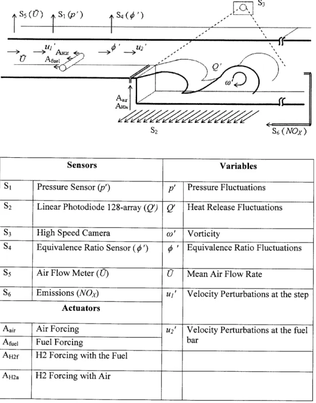
The experimental test-bed is a backward-facing step combustor which provides a sudden expansion with recirculation zone that anchors the flame, as shown in Figure 2-1 and Figure 2-2. It consists of a rectangular stainless steel duct with a cross sectional area 40 mm high and 160 mm wide. Halfway along the length of the combustor, a ramp contracts the channel height from

40 mm to 20 mm, followed by a constant-area section and a sudden expansion back to 40 mm.

The step height is 20 mm. The overall length of the combustor is 1.9 m, with the step located in the middle. The air inlet to the combustor is choked. The exhaust gases are expanded at the end of the chamber. The combustor is equipped with quartz viewing windows. An air compressor supplies air up to 110 g/s at 883 kPa. Propane is used as the primary fuel. Fuel is supplied at several spanwise holes from a fuel manifold located upstream of the step, at 17.5 cm or 35 cm. Fuel is injected in the opposite direction to the flow to improve mixing. The sensors and actuators are positioned as indicated in the figure. In the figure, p' is pressure fluctuations, U is the mean air velocity in the upstream, u,' and u2' are velocity fluctuations at the point of fuel injection and the step, respectively,

Q'

Figure 2-1 Photograph of the MIT backward facing step combustor with various sensors and actuators

Here, I describe the sensors used in the backward facing step combustor. Pressure fluctuation is measured with the Kistler pressure sensors (SI). CH* chemiluminescence, which can be related to heat release fluctuation is measured with the linear photodiode array (S2). 2D

flame structure is measured with a high-speed camera (S3). Equivalence ratio fluctuation is

measured with the laser and photodetector arrangement (S4). The pressure and equivalence ratio

measurements are logged at 1000 Hz by a Pentium III with a dSPACE data acquisition board installed. The linear photodiode array voltages are captured by a Pentium IV with National Instruments data acquisition hardware installed. The overall sample rate is 64 kHz to read all the photodiodes, and each snapshot is captured at 500 Hz. In the following, detailed descriptions of the sensors are provided.

I5

"'airL

Si Pressure Sensor (p') p' Pressure Fluctuations

S2 Linear Photodiode 128-array (Q')

Q'

S3 High Speed Camera wo' Vorticity

S4 Equivalence Ratio Sensor (#') ' Equivalence Ratio Fluctuations

S5 Air Flow Meter (U) U Mean Air Flow Rate

S6 Emissions (NOx) Ul' Velocity Perturbations at the step

Actuators

Aair Air Forcing U2' _{Velocity Perturbations at the fuel}

Afruel Fuel Forcing bar

AH2f H2 Forcing with the Fuel

AH2a _{H2 Forcing with Air}

Figure 2-2 Schematic of the backward facing step combustor with various sensors and actuators

- -.P. OR

S3

2.1.1 Sensors

Pressure Sensors (Si)

Kistler pressure sensors are used to measure the dynamic pressure response from the interior of the combustor. The 6061B ThermoCOMP Quartz Pressure Sensor can measure 0-2.5

bar up to 0-250 bar. It is water-cooled and designed especially for small combustion engines and

for thermodynamic investigations in the laboratory.

Linear Photodiode Array (S2)

CH* chemiluminescence is measured spatially and temporally using a new sensor design

involving a linear photodiode array to capture distributed heat release characteristics [33,34]. An

NMOS linear image sensor (S3901-128Q) is available from Hamamatsu Photonics that provides 128 individual photodiodes in a linear array. Each pixel is 2.5 mm high and 45 um wide. A

flame image can be projected onto this array using the appropriate optics, and a "linear snapshot" can be taken. This has an advantage over a single photodiode, because it provides spatial information. It also has an advantage over a CCD camera, because the data can more easily be streamed to a computer for analysis, and the amount of data can be handled in real-time for control purposes. Each pixel integrates the light intensity over time, and resets when it is read.

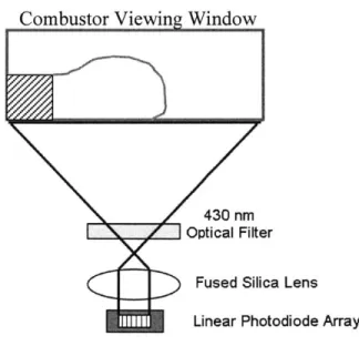
In the experiment, the flame image passes through an optical bandpass filter centered at 430 nm, the wavelength of CH* chemiluminescence (Figure 2-3). Unlike most CCD arrays which have peak sensitivity in the infrared region, the linear photodiode array has a high UV

sensitivity, making it suitable for this application. A bi-convex UV fused silica lens is used to focus the image of the flame onto the chip. The photodiode array has high spatial resolution in the streamwise direction, and integrates the light intensity in the vertical direction.

High Speed Camera (S3)

To capture 2D flame images at a high resolution and high speed, a MotionPro CMOS camera from Redlake is used. The MotionPro system is designed to capture high-speed digital images and deliver them directly into a PC for analysis and documentation with maximum frame resolution of 1280 x 1024 pixels with record rates up to 1000 frames per second. Flexible recording options permit using the PCI-board memory as a circular buffer into which specified pre- and post-trigger frames are recorded, or dividing it into a segmented buffer for multiple session operation.

Combustor Viewing Window

430 nm Optical Filter

Fused Silica Lens Linear Photodiode Array

Figure 2-3 Linear Photodiode Array Sensor (S2) Schematic. The flame image is filtered for CH*

Equivalence Ratio Sensor (S4)

The equivalence ratio sensor uses a laser and a photodetector. The laser emits a beam of light of the wavelength (3.39 pm) that is absorbed by hydrocarbons like methane and propane

[35]. On the other side of the combustor, a detector is installed that is sensitive to that

wavelength of light. When fuel passes through the laser beam, it absorbs some of the laser light and the detector signal is reduced. The intensity of the light can be related to fuel concentration using the Beer-Lambert law, as described by Lee et al. [35].

If= dx

I/Jo =10 0

where I is the intensity of incident monochromatic light, I is the intensity of transmitted light through the absorbing species, e is the decadic molar absorption coefficient (cm2/mol), 1 is the

absorption path length, and c is the concentration of absorbing species (mol/cm3). Figure 2-4

shows the schematic of the device as installed in the step combustor.

InAs Detector I I

Air Flow Sensors (S)

The air mass flow meter is a Sierra Instruments 780S-NAA-N5-EN2-P2-V3-DD-0 Flat-Trak. The maximum flow rate is 173 g/s. The maximum pressure is 827 kPa. The unit is powered by an 18-30 V DC power supply, and it outputs a signal from 0-10 V DC which is proportional to the mass flow rate of the air.

Emission Sensors (S)

Emissions sensors are installed on the rig to provide quantitative measurements of performance characteristics such as NOx concentration and burning efficiency. Fuel modulation is a common stabilization technique. The impact of fuel fluctuations on emissions and efficiency has been measured, but the results have not been used in the feedback loop in a way that optimizes several performance parameters simultaneously at a fixed operating condition [36,37]. Additionally, a study of emissions will provide insight into the possibility that air forcing produces cleaner emissions and more complete burning than fuel modulation. For example, air injection at the step may serve to cool the flame, reducing NOx.

Other uses for this equipment will be to correlate the linear photodiode array with emissions characteristics. For example, it appears that the flame becomes more compact when controlled with air injection. Compact flames are associated with low emissions because of decreased residence time in which to form NOx. Preliminary analysis of linear sensor images appears to show this compact flame shape after control is applied. If a correlation can be made between emissions and linear sensor image, it is possible that the linear sensor could serve as an

An NOx emissions sensor has been installed in the combustor rig. The emissions probe is located 62 cm downstream from the step in the exhaust section. The probe extends 20 mm (half the combustion chamber height) into the chamber, through a 'A-NPT threaded boss. The probe is attached to a Universal Analyzers Model 270S Stainless Steel Heated Stack Filter. The sample line is connected to a Universal Analyzers Model 520 Single Channel Sample Cooler. The cooler brings the sample down to 4 *C. A peristaltic pump removes to the exhaust trench the water that is condensed by this operation. The cooled sample is sent to the Thermo Environmental Instruments Model 42C High Level NO-NO2-NOx Analyzer.

2.1.2 Actuators

In the following, I describe the air and fuel actuators. As indicated in Figure 2-2, the fuel injection occurs several step heights upstream pointing upstream for uniform spanwise mixing. Fuel can be modulated at the fundamental unstable frequency, but since the fuel has time to mix in the streamwise direction before it reaches the flame, the authority of fuel modulation is reduced. Also, this type of actuation introduces a delay between the time the fuel is modulated and the time the fuel encounters the flame, which is not only moving, but also spatially distributed. Air forcing which occurs very close to the dump plane can deliver high authority for actuation energy. Also, adding additional air at the step tends to decrease the temperature, which is favorable for NOx reduction. Detailed description of the air and fuel actuation is in the

Forcing Air (Aair)

Control actuation is accomplished using Dynamco D1B2204 Dash 1 direct solenoid poppet air valves. This valve can supply 1.8 g/s of air when supplied with 689 kPa. The valve is connected to a plenum beneath a 2 mm spanwise slot and 12 mm upstream of the step.

Fuel Forcing (Afuel)

Another valve used for actuation is the Moog D633-7315 AIC Direct Drive Valve (DDV). It has its own built in feedback loop to ensure the spool position using an LVDT. This feedback loop is controlled by the Moog D143-098-013 Single Axis Electronic Controller. This unit is powered by a 48V Condor Power Supply, which also powers the valve. The controller accepts inputs from -10 VDC to 10 VDC.

A transfer function for this valve was determined using system identification. White noise

with a bandwidth of 1000 Hz was the input. The spool position, measured with the LVDT was the output. The spool position is related to mass flow rate by a calibration. The transfer function is

h(s) 0.03837s3 _{- 69.11s} 2 _+1.786

x 10's +1.495 x 10'

S)V(s) s4 +2634s 3 + 7.934x 106S2 +1.034x10 10 _s+3.946x101 2

where rh is mass flow rate (kg/s) and V is the input to the valve (Volt). The Bode plot in Figure

Bode Diagram -90-0 CA -160 Q 20 , 360 -450 1010 10 Frequency (rad/sec)

Figure 2-5 Moog DDV Bode Plot (Bandwidth is 444Hz)

H2 (AH2f & AH2a) Injection

To extend the flammability limit and increase the resistance of the flame to extinction, hydrogen is delivered at 0-9 mg/s through a Sierra Instrument mass flow controller. Hydrogen is either mixed with propane and introduced through the fuel bar, AH2f, or mixed with the air jet and introduced through the slot,

AH2a-2.2

Modeling of Combustion Dynamics

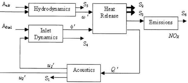
Figure 2-6 shows schematically how various flow, combustion and acoustics mechanisms interact, and their contributions to the combustion dynamics and emissions. This model features the following:

- _{The feedback mechanism that contributes to combustion dynamics, which couples} heat-release dynamics and acoustics.

" The heat-release perturbations that arise due to fluctuations in the equivalence ratio,

#',

and hydrodynamic perturbations, co'.

Optimal actuation for control depends on the mechanism leading to combustion instability. For example, if equivalence ratio fluctuations play a significant role, upstream fuel modulation may work best. On the other hand, if flame-vortex interaction is the governing mechanism, hydrodynamic-based actuation near the step, such as spanwise air injection, would be more effective. A parametric study of the impact of the inlet conditions and the hydrodynamics on the combustion instability is shown in the following sections.

Hydrodynamics H eat 2

Emissions

Afuel _{~ Inlet}

--yDyn ami cs NOX

S4

Ulf ~Acoustics

-Figure 2-6 Schematic diagram of the acoustics, hydrodynamics and heat release dynamics and their interactions.

2.2.1 The Role of the Inlet Dynamics

(Mixture Inhomogeneity)

I first examine the role of fuel/air mixture inhomogeneity,

#'

#'

1 + -_

U

following a convective transport time delay, z,,, determined by the mean mixture velocity, U,

L

and the distance from the point of fuel injection to the burning zone, L , r,, = = [21,38]. U

The convective delay from the point of fuel injection to the burning zone determines the phase between

#

injection location. To determine the impact of the mixture inhomogeneity, or

#

I now consider two cases: I and II, where the fuel bar was located 17.5 cm and 35 cm

upstream from the step, respectively. In both cases, the uncontrolled combustor was operated at different air-flow rates. Figure 2-7 shows the effect of varying the equivalence ratio and Reynolds number on the overall sound pressure level (OASPL). In all these experiments, the excited acoustic mode frequency, fa, was 38 Hz. In Figure 2-7(b), the pressure level almost monotonically increases with the Reynolds number while it is insensitive to the changes in the mean equivalence ratio. In contrast, in Figure 2-7(a), the impact of Reynolds number is non-monotonic showing reduced pressure level at Re = 8500 and increasing suddenly at Re = 9500.

Also at Re = 9500, the pressure level is sensitive to the changes of the mean equivalence ratio.

Similar observations (pressure level increases with the increase in the Reynolds number and is sensitive to the mean equivalence ratio change at high Reynolds number) have been made in Ref.

Re = 9500 Re - -= 6400 Re 7400 Re = 8500 0.55 0.6 0.65 0.7 0.75 0.8 0.85 0.9 0.95

(a) Case I (fuel bar at 17.5 cm)

162 -160 -0 158 -156 154 152 -150 -0.5 Re 8500 - -Re 7400 Re = 6400 Re= 5300 0.55 0.6 0.65 0.7 0.75 0.8 0.85 0.9 0.95 1

(b) Case II (fuel bar at 35 cm)

Figure 2-7 The impact of varying equivalence ratio and Reynolds number on the overall sound pressure level in Cases I and II.

To understand this discrepancy in Cases I and II, this stability map is redrawn with the convective time delay, z,,, as the x axis as shown in Figure 2-8. The convective time delay from

162 -160 -158 -0 158 152 150 0.5 1 1

the fuel injection point to the step is shown in the figure as multiples of r , where r is the acoustic time scale, 1/fa = 26.3 ms. If the instability was controlled by the mixture

inhomogeneity only, a stability band should appear in these maps as the time delay is varied as follows: stable zones when the transport delay is between nir and (n+0.5) r and unstable zones when the delay is between (n+0.5) r and (n+1) z- [21,38]. No changes in the pressure fluctuations were shown in Figure 2-8(b) during these transitions indicating that mixture inhomogeneity does not play a role in Case II. However, in Case I, a pressure drop is observed when the time delay is between r and (n+0.5) r indicating that the equivalence ratio oscillation has a secondary role. This secondary role of the equivalence ratio oscillations in Case I explains the non-monotonic relation between the pressure level and the Reynolds number observed in Fig. Figure 2-7(a).

I further investigated the extent to which the mixture inhomogeneity contributes to

combustion instability. Equivalence ratio oscillations (S4) and the corresponding pressure signal

(Si) are compared in Cases I and II at two different operating conditions. First, at Re = 5300 and

#

Case II due to streamwise diffusion, while significant equivalence ratio fluctuations are observed in Case I. The pressure amplitude is higher in Case I indicating that the equivalence ratio fluctuation increases the pressure oscillations at this operating condition. Note that Case I is in the band between (n+0.5) z and (n+l) r . On the other hand, even without equivalence ratio fluctuations, pressure oscillations are still significant in Case II.

0.9 0.8 0.7 0.6 S0.5 1 1.2 1.4 1.6 1.8

(a) Case I (fuel bar at 17.5 cm)

165 160 155 U U 150 3

Figure 2-8 The impact of Cases I and II.

U U U 3.5 4 U 0 U 4.5 5 5.5 ' tot' /

(b) Case II (fuel bar at 35 cm)

convective time delay on the overall sound pressure level in

The power spectra obtained at a second operating condition, at Re = 8500 and

#

U

a

both cases, where equivalence ratio oscillations may damp out pressure oscillations. While significant equivalence ratio fluctuations are present, Case II has lower values since the fuel bar is positioned further upstream, similar to the Re=5300 experiment. Since the equivalence ratio fluctuations, under these conditions, provide negative feedback, Case I exhibits a lower pressure amplitude. However, both cases show significant pressure oscillations, indicating that the essential mechanism here is not mixture inhomogeneity.

4 i'- Case I L3 Case II 2-C, Q - - - -- -- - -0 0 10 20 30 40 50 Freq(Hz) - Case I 0.4 - ---- Case 11 -\ 0.2 Ji 000 0 10 20 30 40 50 Freq(Hz) (a) Re=5300,

#

Figure 2-9 Pressure (Si) and equivalence ratio (S4) frequency spectra at (a) Re=5300 and

#=0.85

2.2.2

The Role of Hydrodynamics and Flame-Vortex

Interactions

Velocity perturbations can cause repeated shedding of vortical structures at the step. This, in turn, causes the flame shape to change, thereby generating large amplitude of heat release fluctuation. This vortex shedding has a preferred frequency quantified by a Strouhal number St =

fHH / U = 0(0.1) where H is the step height and fH is the frequency in Hz [40]. If the preferred

vortex shedding frequency is near the acoustic mode frequency, fa, the system is more prone to combustion instability.

The strong dependency of combustion instability on the Reynolds number or the mean velocity described above suggests that the primary mechanism causing combustion instability is the hydrodynamics and its interaction with flame. As mentioned before, hydrodynamics has a preferred frequency around fH = 0(0. lU / H). Interestingly, strong instability occurs above

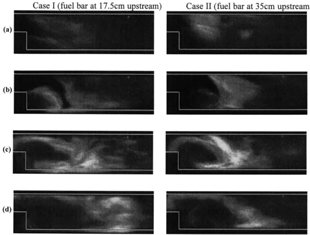
Re=9500 in Case I, and Re=7400 in Case II, as shown in Figure 2-7, in which the preferred frequency is fH =33Hz and 25Hz, respectively, both of which are close to the acoustic frequency, fa,=38Hz. High speed CCD images in Figure 2-10, captured at 500 frames/s, show strong flame-vortex interactions with no noticeable difference in the flame structure between the two cases. These images confirm the role of flame-vortex interactions in the combustion instability mechanism.

Case II (fuel bar at 35cm upstream) (a)

(b)

(d)

Figure 2-10 High speed CCD images of the flame in the backward-facing step combustor at Re=6300 and

#

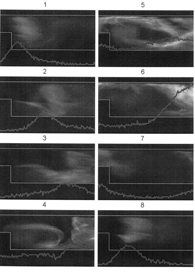
Now, I now show the cyclical flame-vortex interactions using high-speed imaging. We start the analysis of the mechanism from the moment of maximum velocity, according to Figure 2-12

(numbers between brackets correspond to the image number in the figure). Figure 2-11 shows 8 snapshots of the flame from the video record, successive images are separated by 4 ms, that is, the cycles ends almost halfway between (7) and (8) since the cycle time is close to 25 ms. Around the moment of maximum velocity, the flame appears as a vertical front moving downstream of the step (1). Note that due to a combination of local small-scale turbulence and relatively weak variation in the spanwise direction, the flames appear as thick zones. As the

vertical front that accelerates forward on the top half of the channel, and a horizontal front that extends back to the step (2). It is interesting to observe near-extinction at the step during this part of the cycle, apparently due to the high flow velocity/strain rates there (2-3). As the velocity becomes negative, the vertical flame curves slightly forward as it moves faster along the upper wall than the lower wall, and the horizontal flame curves upwards, away from the step, and forms a forward fold closer to the lower walls (4). As the flame departs from the step, it bums vigorously into the inlet channel (4-5). Meanwhile, reactants are trapped in the fold, and in between the fold and the leading curved flame (5). The inception of the fold can be seen in (3-4) clearly, as well as the formation of reactants traps between the fold and the leading vertical flame

(4-5). During this part of the cycle, the curved horizontal flame propagates almost vertically towards the top wall, pushing its leading and trailing edges downstream and upstream, respectively, with the latter migrating further into the inlet channel (4-6). As the velocity emerges from the negative region, the flames surrounding the fold start to converge inward, burning the trapped reactants and closing the gaps (5-6). According to the images, this is the moment of maximum total burning rate. Meanwhile the migration of the trailing edge of the flame into the inlet channel, which started when the velocity delved into the negative domain, is halted as the velocity recovers (5-7). Signs that the flame was pushed back towards the step while the velocity was rising towards its maximum are seen in (7). The cycle is now over, and

1

5

2

6

3

7

4

8

Figure 2-11 High speed CCD images, and the CH* data captured by the linear photodiode, images were captured at 500 Hz, and represent slightly more that one cycle.

41 2 - -0 a-00 4L e + 4-44 -2 Il 0 Js- Pressure 3 --a- Velocity --- Heat Release 4 ' -5 0 5 10 15 20 25 30 Time (ms)

Figure 2-12 Pressure, velocity and heat release rate, with the numbering of the points corresponding to frames in Figure 2-11.

Now, we look closely at the CH* data to correlate the flame geometry, the heat release rate and the pressure. At the beginning of the cycle, the CH* distribution peaks near the step, where the flame front is located at that moment (1). As the flame propagates downstream, the CH* distribution advances with it (2), stretching downstream with a flatter peak as the two parts of the flame become distinguishable (3). Consistent with the video images that shows partial extinction at the step, CH* signal there is near zero (2-3), until the flame is pushed away from the step and into the inlet channel (4). We note the strong correlation between the brightness of the video image and the local CH* signal, confirming the intended use of the former as a surrogate for

near the step, a weak CH* signal starts to appear there, growing slowly in a nearly flat distribution behind the leading peak (4-6), the latter corresponding to a more energetically burning and folding flame that continues its forward propagation (5). One can clearly see the sign of a flame advancing upstream in the CH* image in (5). As the flames converge towards the centers of the folds, the leading peak in CH* rises significantly, heralding the peak heat release rate (6). This is followed by a rapid drop in CH* throughout the channel, except in the inlet channel where a flame is convected back downstream, following its brief early migration there (7). The flame moving downstream the step is again captured in the CH* in (7-8).

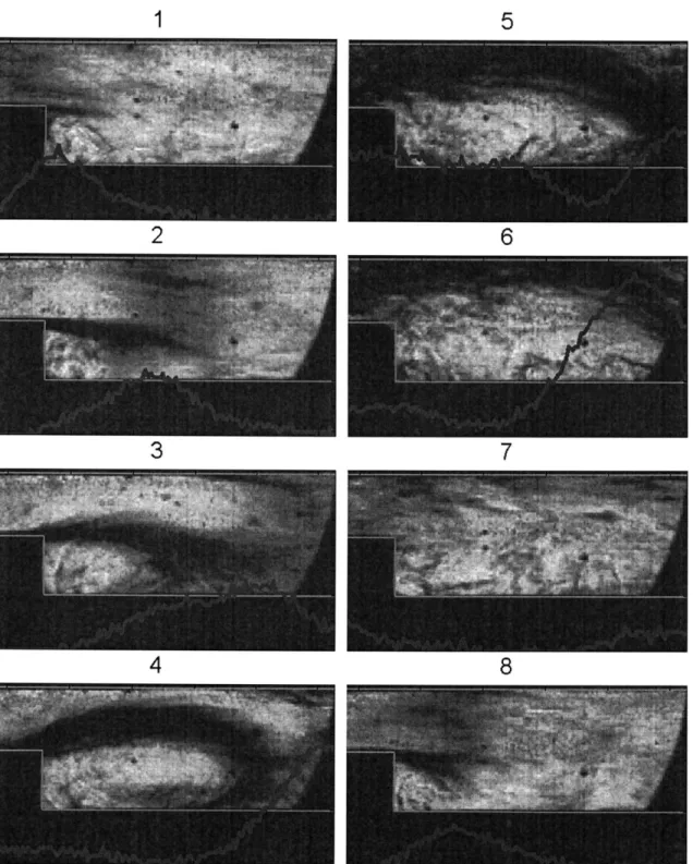
The streamwise integral of CH* represents the instantaneous total heat release rate, shown in Figure 2-12. The fast but more gradual rise in total heat release, followed by the faster drop and slow recovery are clearly depicted in this figure. Because of the dynamics described in the previous paragraphs, the total heat release rate peaks almost 100' ahead of the velocity at the step, at a moment when the velocity near the step is still relatively low but rising. As can be seen in the same figure, and because the dominant acoustic mode is a quarter wave mode, the pressure also leads the velocity by 900, and the pressure and heat release rate are in phase, as expected in an unstable combustor. The mechanism responsible for this coupling is clearly fluid dynamic in nature, and is embedded in how the flow downstream the step causes the flame convolutions shown in Figure 2-11. Next, we examine the Schlieren images to confirm the close relationship between the bright zones in the direct video images and the burning zones, or "thick" flames in the case we analyze here.

before. Statistical variations are responsible for the small differences between the images shown in Figure 2-11 and Figure 2-13, however the similarity is nevertheless very strong. In general, the Schlieren images are better indicators of the flame front surface than the direct video since they capture the density gradient. However they can be affected more by the spanwise averaging, and by heating due to the proximity of walls, e.g., close to the step, which can introduce weak local density gradients in the absence of flames. Despite that, the Schlieren images show strong resemblance to the direct video images, and are also strongly correlated with the CH* distributions.

I 5

2

6

3

7

4

8

Figure 2-13 Schlieren images with CH* data.

2.3 Simultaneous Control of Combustion Instability and

Emissions

In this section, I show open and closed-loop control results using the air jet and H2 addition, in order to simultaneously reduce pressure oscillations and NOx emissions. The fuel bar is located 35 cm upstream of the step. In Section 2.3.1, I consider a static air jet (Aair) near the step and H2 addition to the primary fuel (AH2f). In Section 2.3.2, I show the impact of modulating the air jet (Aair) when it is mixed with hydrogen (AH2a). Primary fuel modulations

(Afuel) at the fuel bar were also attempted, but, as expected from the results of Section 2.2, its

impact on combustion instability was negligible.

2.3.1 Static Air

and H2 injection

(AH2f)

The effect of a steady transverse air jet (Aair), introduced a short distance upstream of the step, on the pressure fluctuations, and the impact of hydrogen addition to the primary fuel (AH2f) in the presence of the transverse air jet as well are now examined. In these tests, the Reynolds number was 6300, with a corresponding average velocity, U = 4.4 m/s. The primary fuel supply

was fixed. The transverse jet air velocity, u,, was varied from 0-8.4 m/s. The hydrogen addition was at 1.6 and 3.2 % of the primary fuel, based on the lower heating value. The baseline equivalence ratio,

#

Figure 2-14 shows OASPL as a function of momentum ratio of main air to cross jet flow,

#8=

#8

Without hydrogen, the flame blows out for 8 < 1.8. However, with 8 > 1.8 the flame became sustainable again, with a pressure reduction of up to 14 dB from the baseline case. With air addition, the overall equivalence ratio was mostly below the nominal flammability limit of propane/air mixture. Moreover, a relatively large momentum in the transverse jet was necessary to reduce the pressure fluctuations and stabilize a flame near the step at yet lower equivalence ratio. Thus, it appears that the impact of the transverse jet is aerodynamic. Studies of simple jet in cross flow show that at small velocity ratios, the jet hardly penetrates into the stream, while as the jet velocity increases, the jet penetration is pronounced and its impact is sustained several jet widths downstream [41]. At high velocity ratios, the jet deflects the primary stream upwards, keeping it away from the lower walls. By deflecting the stream away from the lower wall, less heat is lost to the lower wall and combustion is more adiabatic. Since the transverse jet reduces heat loss and lowering the heat loss promotes burning of lean to very lean mixtures [42], the air jet enables burning at a lower overall equivalence ratio.

Figure 2-14 shows that adding H2 to the primary air stream, in the presence of the transverse jet, has a weak impact on the pressure level before the point of maximum pressure oscillation is reached. Beyond this point, the effect of H2 addition is to support a more stable flame, lowering pressure oscillation and preventing blowout. Moreover, adding hydrogen enables burning over the entire range of the jet mass flow rate (we no longer see blowout around /=1). This is consistent with previous observations that doping hydrocarbons with small amounts