HAL Id: hal-02323403
https://hal.archives-ouvertes.fr/hal-02323403
Submitted on 15 Jun 2020
HAL is a multi-disciplinary open access
archive for the deposit and dissemination of
sci-entific research documents, whether they are
pub-lished or not. The documents may come from
teaching and research institutions in France or
abroad, or from public or private research centers.
L’archive ouverte pluridisciplinaire HAL, est
destinée au dépôt et à la diffusion de documents
scientifiques de niveau recherche, publiés ou non,
émanant des établissements d’enseignement et de
recherche français ou étrangers, des laboratoires
publics ou privés.
Hector Torres, Zhan Su, Dimitris Menemenlis, Sylvie Le Gentil
To cite this version:
Patrice Klein, Guillaume Lapeyre, Lia Siegelman, Bo Qiu, Lee-lueng Fu, et al.. Ocean-Scale
In-teractions From Space. Earth and Space Science, American Geophysical Union/Wiley, 2019, 6 (5),
pp.795-817. �10.1029/2018EA000492�. �hal-02323403�
observations has properties that differ from those related to classical geostrophic turbulence theories. In the last decade, a large number of theoretical and numerical studies has pointed to submesoscale surface fronts (1–50 km), not resolved by satellite altimeters, as the key suspect explaining these discrepancies. Submesoscale surface fronts have been shown to impact mesoscale eddies and the large-scale ocean circulation in counterintuitive ways, leading in particular to up-gradient fluxes. The ocean engine is now known to involve energetic scale interactions, over a much broader range of scales than expected one decade ago, from 1 to 5,000 km. New space observations with higher spatial resolution are however needed to validate and improve these recent theoretical and numerical results.
1. Introduction
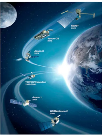
In 1992, a satellite with a high-precision altimeter, Topex/Poseidon (T/P, CNES/NASA), was launched in space to observe the sea surface height (SSH) in all oceans over a range of scales from 100 km to more than 5,000 km. SSH observations, a proxy of surface pressure, were used to retrieve oceanic surface motions using the geostrophic approximation (that assumes an equilibrium between Coriolis and pressure gradi-ents forces). First analyses of T/P observations profoundly revolutionized the field of oceanography. They showed that General Ocean Circulation Models (OGCM) with low spatial resolution were strongly deficient in estimating the kinetic energy (KE) of oceanic motions (Fu & Smith, 1996; Stammer et al., 1996). Wal-ter Munk, testifying before the U.S. Commission on Ocean Policy in April 2002, emphasized that T/P was “the most successful ocean experiment of all time”. In September 2018, over 300 ocean scientists attended a 5-day symposium in Ponta Delgada (Azores Archipelago) to celebrate 25 years of Progress in satellite radar altimetry. Ocean monitoring over more than two decades, using T/P and other satellite altimeters (Figure 1), has led to a major scientific breakthrough responsible of a paradigm shift: all the oceans are now known to be populated by numerous coherent eddies at mesoscale (100–300 km) as illustrated by Figure 2a. Altime-ter observations further emphasize these eddies capture almost 80% of the total oceanic KE of the ocean (Chelton et al., 2011; Ferrari & Wunsch, 2009; Morrow & Le Traon, 2012; Wunsch, 2002, 2009). Although energetic eddies are present everywhere, they are intensified in hot spots associated with major oceanic currents such as the Gulf Stream, the Kuroshio Extension, and the Antarctic Circumpolar Current (see Figure 2b). This vision of a strongly turbulent ocean at mesoscale has been confirmed by recent numerical OGCMs performed with high resolution of a few kilometers (see Figure 3).
Due to the high vertical stratification of the open ocean and the Earth rotation, oceanic motions at scales larger than 100 km are geostrophic and quasi-horizontal (Vallis, 2017); that is, vertical motions at these scales are very weak. So it is not surprising that the ocean mesoscale turbulence (OMT) revealed by satel-lite altimeters was then expected to obey the properties of geostrophic turbulence (GT), described in many
Correspondence to:
P. Klein,
Citation:
Klein, P., Lapeyre, G., Siegelman, L., Qiu, B., Fu, L.-L., Torres, H., et al. (2019). Ocean-scale interactions from space. Earth and Space Science, 6, 795–817. https://doi.org/10.1029/ 2018ea000492
Received 5 OCT 2018 Accepted 3 APR 2019
Accepted article online 10 APR 2019 Published online 22 MAY 2019
©2019. The Authors.
This is an open access article under the terms of the Creative Commons Attribution-NonCommercial-NoDerivs License, which permits use and distribution in any medium, provided the original work is properly cited, the use is non-commercial and no modifications or adaptations are made.
Figure 1. Existing and future satellite altimeters (see https://sealevel.jpl.nasa.gov/).
theoretical and numerical studies starting with Charney (1971; see, e.g., Hua et al., 1998; Hua & Haidvogel, 1986; McWilliams, 1989; Rhines, 1975, 1979).
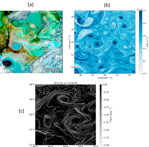
Because of the specific impacts of the rotation and vertical stratification, GT properties strongly differ from the classical 3-D turbulence properties (Tennekes & Lumley, 1974). A first difference is the existence in GT of an inverse KE cascade, driven by the nonlinear interactions between eddies, such that KE fluxes from the scales of eddy sources (mostly explained by baroclinic instability) toward larger scales (for which Rossby wave dispersion starts to dominate and nonlinear interactions weaken). Such inverse KE cascade is con-comitant with the nonlinear merging between coherent eddies giving rise to larger ones (Vallis, 2017). As a consequence, the resulting eddy fluxes significantly increase the total KE and further strengthen large geostrophic eddies by making them more coherent with a longer life time and ultimately leading to the emergence of zonal jets when Rossby wave dispersion becomes significant (Panetta, 1993; Rhines, 1975). Such inverse KE cascade is not observed in 3-D turbulence that only experiences a direct KE cascade from KE sources to smaller scales and therefore to dissipation scales (Tennekes & Lumley, 1974). A second differ-ence is the direct cascade of dynamically passive or active tracers toward small scales driven by geostrophic eddies (Lapeyre et al., 2001). Through the action of stretching and folding, geostrophic eddies generate long and thin filaments of tracers (as illustrated in the ocean by the chlorophyll or Ertel potential vorticity maps; see Figures 4a and 4b) that eventually mix with their surrounding environment (Ledwell et al., 1993; Pierrehumbert et al., 1994). Maps of Finite Size Lyapunov Exponents, or FSLE, are a usual index to mate-rialize these stretching and folding processes (see Figure 4c). The associated mechanisms, called chaotic advection (Aref, 1984; Lapeyre, 2002), make mixing much more efficient than expected from the classical diffusion paradigm used in 3-D turbulence, by at least 2 to 3 orders of magnitude (Garrett, 1983).
Using the GT framework has been illuminating to understand how oceanic mesoscale eddies, observed by satellite, control the global meridional heat transport (Hausmann & Czaja, 2012) and how they shape the large-scale ocean circulation through the inverse KE cascade (Hurlburt & Hogan, 2000). The GT frame-work has also been used to understand how OMT drives the three-dimensional dispersion and mixing of
Figure 2. (a) Trajectories of cyclonic (blue lines) and anticyclonic (red lines) eddies (estimated from altimeter data)
over the 16-year period, October 1992 to December 2008, for lifetimes>16 weeks (from Chelton et al., 2011). (b) Map of the standard deviation of eddy SSH amplitude (in centimeters; from Chelton et al., 2011, used with permission.) SSH = sea surface height.
tracers, such as nutrients and therefore the biological diversity and carbon storage (d’Ovidio et al., 2010; McGillicuddy Jr, 2016). Mezic et al. (2010) applied GT ideas to improve the forecast of pollutants dispersion using altimeter observations. They used these ideas for the forecast of the oil spill dispersion after the Deep Water Horizon accident in the Gulf of Mexico (see also Poje et al., 2014). Assimilation of satellite altimeter observations and in situ global data sets (such as the ARGO float dataset) in numerical models has led to the fast development of operational oceanography (Chassignet et al., 2018; Le Traon, 2013). Some assimilation techniques make use of the GT framework to better represent the OMT impacts on tracers. For example, Gaultier et al. (2012) proposed to assimilate the stretching (or strain) field (i.e., the second-order spatial derivatives of SSH) instead of simply assimilating SSH. These authors showed how this idea helped to much better predict the chlorophyll dispersion by mesoscale eddies.
Figure 3. Instantaneous snapshot of the kinetic energy in the global ocean, from a global Estimating the Circulation
and Climate of the Ocean (ECCO) numerical simulation ((1/48)◦degree resolution in the horizontal and 90 vertical levels). (See https://science.jpl.nasa.gov/projects/ECCO–ICES/).
Figure 4. (a) Satellite image of the chlorophyll in the Southern Ocean (see https://earthobservatory.nasa.gov/). (b) Map
of the Ertel potential vorticity in the Southern Ocean from the global ECCO numerical simulation (see above). Ertel potential vorticity is a dynamical active tracer conserved on a 3-D Lagrangian trajectory. (c) Map of the Finite Size Lyapounov Exponents (FLSE) in the Southern Ocean estimated using sea surface height from the global ECCO numerical simulation ((1/48)◦resolution in the horizontal and 90 vertical levels; see https://science.jpl.nasa.gov/ projects/ECCO-IcES/). FSLE are an index of the dispersion of tracers and particles by geophysical eddies (with a size of less than 100 km on this map; see more details about FSLE in d’Ovidio et al., 2010).
Still, some disconcerting discrepancies between OMT properties diagnosed from SSH observations and what is expected from GT theory are not fully understood (Morrow & Le Traon, 2012) as detailed in section 2. One of the key suspects, highlighted by numerical models with high spatial resolution, is the impact of smaller scales not resolved by existing satellite altimeters, in particular surface frontal structures with a 1- to 50-km width (called submesoscales in the present paper) for which the geostrophic approximation still works, but only at zero leading order. The numerous numerical and theoretical studies devoted to submesoscales and their interactions with mesoscale eddies of the past 15 years have led to startling discoveries discussed in section 3. One of them points to the extension of the inverse KE cascade to scales down to 30 km, that is, in a regime where frontal processes are beginning to take place. This suggests that the oceans are even less diabatic and more inertial than we thought; that is, fluxes of any quantities (including KE) are much less controlled by diffusivity or viscosity (which leads to irreversible downgradient fluxes) and more by nonlinear interactions that can lead to reversible up and downgradient fluxes. Mesoscale and submesoscale motions with scales down to 30 km should be observable by the forthcoming Surface Water and Ocean Topogra-phy (SWOT) altimeter mission (Fu & Ferrari, 2008) described in section 4. However, one challenge to meet to analyze these future observations is that balanced motions (BMs) with scales smaller than 100 km are entangled with another class of motions, the internal gravity waves (IGWs), as discussed in section 5. The most recent results using numerical models with the highest spatial resolution allowed by available petascale computers (Chassignet & Xu, 2017, Lévy et al., 2010, Su et al., 2018, Torres et al., 2018; Figure 3) highlight that ocean-scale interactions, involving scales down to 1 km, affect the ocean dynamics in
counter-Figure 5. Frequency (cycle/day) and zonal wavenumber (cycles/km) spectrum of sea surface height variance estimated
from altimeter data. (left) A two-dimensional spectrum plotted on a linear power scale, smoothed in frequency and zonal wavenumber. (right) The logarithm of the power. Dashed curves indicate the barotropic and first baroclinic mode dispersion curves of Rossby waves. Dash-dotted lines are the corresponding curves for the unit aspect ratio. The “nondispersive line” defined in the text lies along the ridge of maximum energy density and is closely approximated by the dotted white line (in the red area of the right panel) with a slope of 4 km/day (from Wunsch, 2009, 2010, © La Societe Canadienne de Meterologie et d'Oceanographie, reprinted by permission of Taylor&Francis Ltd, www. tandfonline.com on behalf of La Societe Canadienne de Meterologie et d'Oceanographie.).
intuitive ways, as illustrated by some examples in section 6. Submesoscale structures in one region not only impact ocean dynamics locally but also impact ocean dynamics in remote regions (Chassignet & Xu, 2017; Lévy et al., 2010). The implication is that understanding how the ocean engine works, over such a large range of scales, requires a numerical strategy involving large domains and employing the highest spatial resolution. However, as Carl Wunsch put it during the OSTST meeting in Lisbon in 2010: “Increased resolu-tion in ocean models needs to be accompanied by higher resoluresolu-tion observaresolu-tions” on a global scale, which is presently a real challenge, as discussed in section 7. Such observations are indeed highly needed to question theories and models in order to improve our understanding of the ocean dynamics, which eventually will lead to new theories and models. The synergy of using observations from different satellite missions should help to better understand the dynamics involved in this broad range of scales, as discussed in section 7. The purpose of this paper is not to provide a thorough and comprehensive review of the important contri-bution of satellite altimeters to the knowledge of the OMT but rather to point to the missing mechanisms that can potentially improve this knowledge. The paper mostly focuses on the upper ocean (from the sur-face down to ∼1,000 m) in extra-equatorial latitudes. Equatorial dynamics are discussed in another paper in this issue (see Menesguen et al., 2019).
2. Ocean Mesoscale Turbulence and Theory of Geostrophic Turbulence
Present altimeter observations concern spatial scales (larger than 70–100 km) for which the associated motions are characterized by a Rossby number (defined as Ro≡ U∕fL with U and L, respectively, a veloc-ity and length scales, and f the Coriolis frequency) smaller than 1. This means that these surface motions are either in geostrophic balance (i.e., a balance between Coriolis and horizontal pressure forces leading to
−𝑓 ⃗k × U = −g∇SSH, with ⃗k the vertical vector) or in gradient wind balance (a balance that, in addition,
involves the nonlinear terms, i.e., U.∇U − 𝑓 ⃗k × U = −g∇SSH; Vallis, 2017).
BMs diagnosed from satellite altimeter observations now concur with the idea that the oceans are fully tur-bulent, involving strongly interacting mesoscale eddies and giving rise to significant energy transfers across scales. This turbulent character was revealed by one of the first𝜔-k spectrum (with 𝜔 the frequency and k the horizontal wavenumber) of ocean variability estimated from SSH observations (Wunsch, 2009, 2010). As illustrated in Figure 5, the maximum of the SSH variance does not follow the dispersion relation curves asso-ciated with linear Rossby waves. Rather, it lies approximately along a “nondispersive” line, c.k + 𝜔 = 0 (with
k < 0), corresponding to an eddy propagation speed of c ≈ 4.6 cm/s (close to the values found independently
by Fu, 2009). This finding highlights the strong nonlinear character of mesoscale eddies, confirmed later on by the study of Chelton et al. (2011). All these results point to the existence of an energetic OMT expected
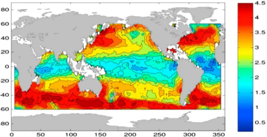
Figure 6. Global distribution of the spectral slopes (k−n) of sea surface height wavenumber spectrum in the
wavelength band of 70–250 km estimated from the Jason-1 altimeter measurements. The color scale is related to values of n (from Xu & Fu, 2012, © American Meteorological Society. Used with permission.).
to share the GT properties described in Charney (1971), Hua and Haidvogel (1986), McWilliams (1989), and Hua et al. (1998). However, some intriguing discrepancies between OMT and GT properties quickly emerged. Let us comment on two of them.
The first one concerns the KE spectral slope estimated from satellite altimetry. Based on GT theory, the KE spectrum should scale in k−3(Charney, 1971). However, KE spectra deduced from altimeter observations using the geostrophic balance do display a linear slope in log-log space in the scale range 100–300 km, but with a power law varying between k−2and k−3. This discrepancy, early noted by Fu (1983), was first attributed to altimeter noise. But more careful estimations, using a larger set of altimeter observations, by Le Traon et al. (2008), confirmed the k−2slope. Such slope for the KE spectrum suggests that smaller eddies resolved by satellite altimeters are more energetic than predicted by GT. Xu and Fu (2012) recently highlighted an even more complex picture displaying a strong regional dependency of the SSH spectral slope (Figure 6). On one hand, in many high KE regions, the resulting KE spectral slopes vary between k−3and k−2. On the other hand, in low KE regions, such as in the eastern part of ocean basins, the spectral slope is even flatter than k−2, which is unrealistic in terms of geostrophic motions (Xu & Fu, 2012). The consensus that presently emerges is that this diversity of spectral slopes is not due to altimeter noise but is due to physical mechanisms other than those involved in GT that vary seasonally and regionally (Dufau et al., 2016; Xu & Fu, 2012).
Another discrepancy concerns the KE fluxes or the inverse KE cascade. As mentioned before, GT theory suggests that mesoscale geostrophic eddies should experience an inverse KE cascade, with KE fluxing from the scales of eddy sources (50–100 km for the ocean) to the scales of the most energetic eddies (Le∼250–300
km for oceanic mesoscale eddies; Charney, 1971; Hua & Haidvogel, 1986; Hua et al., 1998; McWilliams, 1989; Rhines, 1975. Studies by Smith, 2007 and Tulloch et al. 2011), using altimeter observations and in situ data, confirmed the factor 3 to 4 between the eddy source scales and scales of the most energetic eddies, suggesting an inverse KE cascade over a broad scale range. However, the first KE fluxes estimated from altimeter observations by Scott and Wang (2005) were not consistent with this picture. Rather, these authors found an inverse KE cascade over a narrower scale range, that is, starting only at wavelengths larger than 150 km, the smaller wavelengths (including the eddy source scales) experiencing a direct KE cascade (Figure 7a). Some studies, such as Arbic et al. (2012) and Arbic et al. (2013), questioned the contribution of smaller scales, unresolved by altimeter observations, for the transfer of energy between scales. Using an OGCM with a (1/32)◦spatial resolution, they showed that the scale range and magnitude of the inverse KE cascade are strongly sensitive to the resolution of small scales: when small scales are taken into account, the inverse KE cascade involves a much broader scale range involving smaller scales. Thus, KE at scales unresolved by satellite altimeters may contribute to KE fluxes that strengthen eddies resolved by altimetry through the inverse KE cascade. This contribution of unresolved scales seems to be in agreement with the ∼ k−2spectral slope previously mentioned and as further detailed in section 3. Note that, in terms of inverse KE cascade, Arbic et al. (2012) are the first authors to show that OMT experiences an inverse KE cascade in frequency as well.
Figure 7. (a) Spectral kinetic energy flux versus total wavenumber estimated from altimeter data. Black curve using
sea surface height on a32 × 32grid, red curve using sea surface height on a64 × 64grid, blue curve using velocity on a64 × 64grid. Positive slope reveals a source of energy. The larger negative lobe reveals a net inverse cascade to lower wavenumber. Error bars represent standard error. (From Scott & Wang, 2005, © American Meteorological Society. Used with permission.) (b) Spectral kinetic energy flux (from numerical simulations) integrated over the upper 200 m for a flow forced by the Charney instability (and therefore involving submesoscale frontal structures; solid black) and a flow forced by Phillips instability (and therefore with no submesoscale structure; solid gray). Uncertainty is represented as dotted lines based on the assumption that the 360-day run corresponds to 12 independent realizations. In the inset, the vertical axis is zoomed in the range of large wavenumbers to better emphasize the forward cascade. (from Capet et al., 2016, © American Meteorological Society. Used with permission.) Similar results are found in Sasaki et al. (2014). For larger scales, OMT properties appear to match GT properties. One example concerns the arrest of the inverse KE cascade which leads, from GT, to the emergence of alternating zonal jets with a width close to the Rhines scale, that is, the scale at which the Rossby wave dispersion starts to dominate and the nonlinear interactions weaken (Hua & Haidvogel, 1986; Panetta, 1993; Rhines, 1975; Vallis, 2017). Maximenko et al. (2005, 2008) tested their existence using satellite altimeter observations averaged over more than 10 years (which filters out mesoscale eddies). Results reveal the presence of multiple zonal jets, with an east-west velocity direction alternating with latitude, in many parts of the world oceans (Maximenko et al., 2005, 2008). At midlatitudes, jets have often a meridional wavelength close to or larger than 300 km, that is, close to the Rhines scale.
The second example concerns the vertical eddy scale. The combination of SSH and moorings observa-tions (Wunsch, 2009, 2010; Wortham & Wunsch, 2014) shows that roughly 40% of the KE at mesoscale is barotropic in nature, with about another 40% lying in the first baroclinic mode. Since the buoyancy fre-quency, N(z), in the ocean is surface intensified, the KE contribution of the first baroclinic mode is also intensified there, leading to the conclusion that KE inferred from altimeter observations is primarily (but not wholly) in the first baroclinic mode (Hua et al., 1985; Wunsch, 2010). In other words, KE at mesoscale con-centrates in the first 500–1,000 m below the surface in agreement with the GT theory and numerical studies
of Fu and Flierl (1980), Hua and Haidvogel (1986), and Smith and Vallis (2001). As found by these studies, the energy is rapidly transferred from high to lower baroclinic modes, leading to an inverse KE cascade that is not only 2-D but also 3-D in space.
As a summary, altimeter observations reveal that OMT shares some similarities with GT but also point to some discrepancies. Present studies indicate that many of these discrepancies, in particular in high KE regions, are likely explained by the missing contribution of unresolved small scales of BMs that concern submesoscale density fronts at the ocean surface as discussed in section 3. On the other hand, discrepancies in low KE regions seem to be due to the contribution of IGWs, as discussed in section 5.
3. Ocean Mesoscale/Submesoscale Turbulence: A New Paradigm Involving
Submesoscale Fronts
It has been acknowledged for a long time that the formation and development of atmospheric storms (the equivalent of ocean mesoscale eddies) can only be understood by taking into account density fronts with smaller scales at the troposphere's boundaries (i.e., the Earth surface and the tropopause). The turbulence associated with this boundary frontal dynamics (Hoskins, 1976) was first studied by Blumen (1978) who developed a surface quasi-geostrophic (SQG) theory. SQG theory assumes zero potential vorticity in the fluid interior with the flow being driven by the time evolution of density at the boundaries, leading to intense fronts at scales smaller than the Rossby radius of deformation (Held et al., 1995). SQG turbulence was used to explain the dynamics of the atmospheric tropopause by Juckes (1994) and Hakim et al. (2002).
The impact of surface density fronts at submesoscale on the OMT started to be questioned only in the early 2000s. Subsequent studies were based on the theoretical results obtained for the atmosphere and in partic-ular on the SQG theory. Although it has obvious limitations and shortcomings, such as an underprediction of the amplitude of subsurface velocities (see LaCasce, 2012 for example), SQG dynamics coupled with GT à la Charney (Tulloch & Smith, 2006) has been a helpful dynamical framework to understand the interac-tions between submesoscale dynamics and mesoscale eddies. But later studies have revealed a more complex picture as detailed below.
3.1. Surface Frontal Dynamics
Within the oceanic context, early 2000s numerical models (Lévy et al., 2001) that resolved scales down to 10 km pointed to an appealing property of surface density fronts at submesoscales. These fronts are intimately associated with large vertical velocities extending from surface down to a depth of at least 300–500 m, with values much larger than those reported for 3-D GT but close to those reported for SQG turbulence (Klein & Lapeyre, 2009). Two other properties of SQG turbulence that address the discrepancies mentioned before, led to studies focused on near-surface fronts at submesoscales and their interactions with mesoscale eddies using the SQG paradigm (starting in 2006 with LaCasce and Mahadevan (2006), Lapeyre and Klein (2006) and Lapeyre et al. (2006)): the first property is the k−5/3KE spectrum of SQG turbulence (Blumen, 1978; Held et al., 1995), instead of a k−3spectrum for 3-D GT or 2-D turbulence. The second property is that an SQG flow experiences an inverse KE cascade (Capet et al., 2008), starting at submesoscale, indicating that submesoscale fronts may energize larger scales.
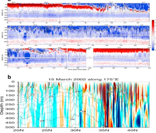
Later on, a large number of studies quickly revealed that the production of oceanic submesoscale fronts and their interactions with mesoscale eddies may result from mechanisms different from SQG. Thus, Boccaletti et al. (2007) and Fox-Kemper et al. (2008), among others, revisited previous results from Stone (1966) who described baroclinic instabilities within atmospheric boundary layers. They showed that similar instabilities occur within the oceanic surface mixed layer during winter when it is deep. These mixed-layer instabili-ties lead to the production of numerous intensified submesoscale fronts during this period. Seasonality of submesoscale fronts has been confirmed by in situ observations in the North Atlantic (Callies et al., 2015; Thompson et al., 2016; see Figure 8a) and further detailed by several oceanic numerical models at a basin scale (Chassignet & Xu, 2017; Mensa et al., 2013; Qiu et al., 2014; Rocha, Gille, et al., 2016; Sasaki et al., 2014 and also, J. Le Sommer, personal communication, June, 2018). Klein et al. (2008), Roullet et al. (2012), Qiu et al. (2014), and Capet et al. (2016) pointed to another mechanism, a coupled surface/interior baroclinic instability (the so-called Charney, 1947, instability), able to produce submesoscale fronts near the surface (a mechanism also emphasized by Tulloch et al., 2011). Recently, Barkan et al. (2017) further discussed how the high-frequency part of the wind forcing can also trigger frontal instabilities at submesoscale.
Figure 8. (a) Yearlong time series of Ertel potential vorticity (10−9s−3), calculated from glider data in the Northeastern Atlantic ocean. The time series is divided into (top) fall, (middle) winter, and (bottom) spring-summer periods; calendar dates (dd.mm) are provided along the top of the panels. The black contour is the mixed layer depth. (from Thompson et al., 2016, © American Meteorological Society. Used with permission.) (b) Meridional section of vertical velocity in the Northwestern Pacific (from a numerical simulation): vertical velocity (color, m/day), potential density (black contour), and Mixed-Layer Depth (MLD) (green line). (from Sasaki et al., 2014).
In most of these studies, the driving mechanism for the production of submesoscale fronts is the action of the geostrophic strain on the surface buoyancy gradients which leads to intensified horizontal fronts and strong vertical motions. It turns out that these fronts, whatever mechanisms that produce them, have properties close to SQG turbulence, such as a tight relation between buoyancy and relative vorticity (see Figure 7 of Klein et al., 2008) and an ∼ k−2(i.e., close to k−5/3) KE spectrum slope associated with an inverse KE cascade starting at submesoscales. Some extensive reviews have been recently dedicated to surface frontal dynamics at submesoscale in the oceans such as those by McWilliams (2016) and Lapeyre (2017).
3.2. Coupling Between Surface Frontal Turbulence and OMT: A New Energy Route Involving Submesoscales
Whereas mesoscale eddies capture most of the horizontal motions (horizontal KE), submesoscale fronts are now known to capture most of the vertical velocity field (vertical KE) in the upper ocean, that is, in the first 500–1,000 m below the surface (Klein et al., 2008; McWilliams, 2016,Thompson et al., 2016; see also Figure 8b). This important property, that can be demonstrated using SQG and QG arguments (see Figure 10 in Klein & Lapeyre, 2009), has been confirmed by several numerical models at a basin or global scale (Sasaki et al., 2014; Su et al., 2018; see Figure 8b). As Ferrari (2011) puts it “these small-scale surface fronts are the equivalents of the thin ducts in the lung called aveoli that facilitate the rapid exchange of gases when breathing.” Near-surface submesoscale fronts are now thought to be the preferential path of heat, nutrient, and other gas exchanges between the ocean interior and surface. In addition, vertical velocity associated with submesoscale fronts impacts the energy route. Indeed, vertical fluxes of buoyancy (or density) driven by submesoscale frontogenesis near the ocean surface correspond to a transformation of potential energy (PE) into KE that scales as w𝜌 ∝ |∇𝜌|2with w the vertical velocity and𝜌 the density (see Capet et al., 2008;
Fox-Kemper et al., 2008; Lapeyre et al., 2006 for this scaling). Since the density spectrum near the surface has a k−2slope (Fox-Kemper et al., 2008; Sasaki et al., 2014), and therefore ∇𝜌 has a flat spectrum, this means
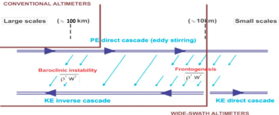
Figure 9. Schematic of the energy route involving mesoscales and submesoscales. PE is known to experience a direct
cascade from large to small scales because of the eddy stirring (see upper line). The new energy pathway involving submesoscales includes a transformation of PE into KE at fine scale (∼10–20 km) due to frontogenesis and an inverse KE cascade over a wide spectral range (see lower line). Conventional satellite altimeters only capture the classical energy pathway involving interior baroclinic instability at mesoscale (down to 100 km). Future wide-swath altimeters, such as Surface Water and Ocean Topography, should capture the energy pathway involving finer scales (down to
∼10–20 km). PE = potential energy; KE = kinetic energy.
that w𝜌 is captured by the smallest scales (Klein & Lapeyre, 2009). In terms of energy exchanges, the picture that emerges is a tight interaction between oceanic mesoscale eddies and submesoscale motions that lead to more energetic mesoscales eddies. Indeed, as sketched in Figure 9 (upper part), mesoscale eddies stir and stretch the surface density field leading to the production of surface density anomalies at smaller and smaller scales (a process called direct PE cascade) and therefore to the production of fronts at submesoscale. These submesoscale fronts give rise to vertical fluxes of density, and therefore to a transformation of PE into KE at submesoscale. A large part of this KE at submesoscale is then transferred to mesoscale eddies through the inverse KE cascade (Capet et al., 2016; see Figure 7b and lower part of Figure 9).
The energy route involving submesoscale density fronts can be coupled with the energy route à la Salmon (Salmon, 1980), that is, the one associated with GT involving a transformation of PE into KE at the Rossby radius of deformation (i.e., at mesoscale) through baroclinic instability, as sketched in Figure 9. Such cou-pling has been proposed by several studies (Callies et al., 2016; Tulloch & Smith, 2006). The resulting energy route and the associated ocean-scale interactions now include a much broader range of scales (Figure 9) with the inverse KE cascade now starting at submesoscales, as shown by Capet et al. (2016; Figure 7b). This inverse KE cascade over a broad scale range reconciles with the findings of Smith (2007) and Tulloch et al. (2011) and is also consistent with the results from Arbic et al. (2013) mentioned before. As sketched in Figure 9, future wide-swath satellite altimeters (such as SWOT; see section 4) should resolve not only the eddy generation scales but also a large part of submesoscales and therefore this inverse KE cascade. The inverse KE cascade over such a broad scale range has been questioned when the strong ageostrophic character of submesoscale fronts is taken into account (see Molemaker et al., 2010 for a discussion). So far, most numerical models at a basin or a global scale, using primitive equations with resolution up to 1–3 km (Capet et al., 2016; Mensa et al., 2013; Qiu et al., 2014; Rocha, Chereskin, et al., 2016; Rocha, Gille, et al., 2016; Sasaki et al., 2014; Su et al., 2018), take into account this ageostrophic character. They point to a transition scale, between the inverse and the direct KE cascade, close to 20–30 km in terms of wave-length depending on the season and the oceanic region (see again Figure 7b). Many of these studies further show how energetic submesoscale fronts in winter can impact the mesoscale eddy field in spring and sum-mer because of the time lag associated with the inverse KE cascade (see Qiu et al., 2014; Sasaki et al., 2014). Thus, mixed-layer instabilities at submesoscale in winter appear to provide an explanation of the puzzling seasonality of mesoscale KE (displaying a KE peak in spring/summer) observed in altimeter observations (Sasaki et al., 2014; Zhai et al., 2008). Numerical models also reveal a significant seasonality of the velocity wavenumber spectrum, displaying a k−2slope in winter and k−3slope in summer. These results are consis-tent with the in situ data analysis of Callies et al. (2015) in the Gulf Stream region, of Qiu et al. (2017) in the Western Pacific, and with the results from Xu and Fu (2012) and Dufau et al. (2016) based on a reanalysis of conventional altimeter observations.
Figure 10. The minimum wavelengths (km), Ls, expected to be resolved by Surface Water and Ocean Topography (a), in ASO (b), and in FMA (c). The seasonal change (ASO-FMA) is shown in panel (d). These wavelengths have been estimated using a numerical simulation (from Wang et al., 2019, © American Meteorological Society. Used with permission.) ASO = August-September-October; FMA = February-March-April.
4. Observational Challenges Using Future Satellite Altimetry (SWOT)
The theoretical and numerical results, of the last decade, on submesoscale BMs and their impacts on mesoscale eddies, need to be confronted and confirmed by observations. Since these results emphasize a strong regionality and seasonality, observations have to be global in space and continuous in time over sev-eral years. Only satellite altimetry can achieve this goal. Existing conventional radar altimetry has, however, two limitations. First, the instrument noise exceeds signal strength at wavelengths shorter than 50–70 km. Second, only one-dimensional SSH is profiled along the satellite ground tracks. To advance the observational capability, and in particular to capture a broader scale range of BMs, a wide-swath altimeter mission, SWOT, has been designed to observe SSH with a higher spatial resolution and in two dimensions (Fu & Ferrari, 2008). This is possible using the radar interferometry technique (Fu & Ubelmann, 2014; Rodríguez et al., 2018). The SWOT resolution is expected to be about 15 km over 68% of the ocean, assuming 2-m significant wave height, along a swath with a ∼ 120 km width (see https://swot.jpl.nasa.gov/mission.htm).
However, before diagnosing BMs at scales smaller than 50–70 km using SWOT observations, several chal-lenges have to be met. First, the measurement noise increases with significant height of surface waves and this noise is known to be seasonally and geographically dependent. Second, at wavelengths shorter than ∼ 100km, the SSH signals of internal tides and IGWs may become comparable to those of submesoscale BMs. This entanglement of the balanced and wave motions is discussed in more details in the next section. It leads to a complicated spatial and temporal variability of the scales of BMs resolvable by SWOT (Qiu et al., 2018). Using an OGCM with a high spatial resolution (similar to the one leading to Figure 3), Wang et al. (2019) studied the scales expected to be resolved by SWOT after taking into account the noise issues. Shown in Figure 10 are global maps of the minimum wavelengths, Ls, possibly resolvable by SWOT. In the tropics,
the measurement noise is generally the lowest owing to the small height of surface waves, leading to the highest resolution (Ls < 20 km), which is also attributable to the shallow spectral slope of the SSH (Xu & Fu, 2012). In regions of the Southern Ocean with moderate mesoscale KE, the measurement noise is the worst owing to the large height of surface waves, which leads to the poorest resolution (Ls ∼40–50 km).
Figure 11. (From Torres et al., 2018). (i) Schematic spectrum displaying the multiple dynamical regimes: Mesoscale
Balanced Motions (MBM), Submesoscale Balanced Motions (SBMs), “Unbalanced Submesoscale Motions” (USMs) and IGWs. Additionally, the scheme shows the linear dispersion relations of the first 10 baroclinic modes for IGWs (in green, upper part) and of baroclinic mode one for Rossby waves (in green, lower left corner). (ii)
Frequency-wavenumber spectra of KE (EKE [m2/s2/(cpkm×cph)]) corresponding to the Kuroshio-Extension region, in winter. The spectrum, estimated from a numerical simulation, is multiplied by k and𝜔. (ii) (a) Frequency spectra. (b) Wavenumber spectra. (c) Frequency-wavenumber spectra (from Torres et al., 2018). Three horizontal bands with frequencies close to tidal (semidiurnal and diurnal) and inertial frequencies span a larger range in the small scales band. Integrating this𝜔 −kspectrum over the k range or𝜔range leads to the frequency spectrum (a) or the wavenumber spectrum (b), respectively.
However, in other regions of the Southern Ocean with strong mesoscale and submesoscale eddies, such as downstream the Kerguelen Plateau, the resolution is much better (Ls < 30 km). As shown in Figure 10d,
during the winter seasons, the resolution is generally poorer than summer north of 40◦S because of the effects of surface waves. The situation south of 40◦S is different. During winter, the mesoscale energy is so high that the signal strength overcomes the increased noise, leading to higher resolution than summer. In addition to the variability of the spatial resolution, the temporal sampling of SWOT is also challenging. Owing to the 120-km swath, it will take 21 days to map the world oceans, with the number of repeat obser-vations varying from two in the tropics to six at latitudes of 60◦. Given the short time scales of the ocean variability at small scales, this temporal sampling poses another challenge to reconstruct coherent patterns of SSH over time. To meet this challenge, it is desirable to make use of high-resolution assimilative models guided by geophysical fluid dynamics argument (Ubelmann et al., 2015) and also by an a priori knowledge of the relative contribution of BMs and IGWs (see Qiu et al., 2018; Torres et al., 2018). These last two stud-ies should help analyze the regionality and seasonality of observations at submesoscales. Given the global high-resolution measurements of SSH signals down to O(15 km), the SWOT mission should provide us with unprecedented information about the evolution of small-mesoscale and submesoscale features and the possibility to reconstruct the upper ocean circulation such as relative vorticity and vertical velocity associ-ated with BMs (Klein et al., 2009; Qiu et al., 2016). By disentangling the SSH signals of BMs versus IGWs (see section 5 below), the SWOT-measured SSH data may also allow us to potentially explore interactions between the balanced and unbalanced motions.
5. BMs and IGWs
As mentioned before, ocean currents with scales equal to or less than 300 km involve not only BMs but also IGWs whose properties significantly differ from BMs. IGWs include wind-forced near-inertial waves, with frequencies close to f and coherent internal tides with diurnal and semidiurnal frequencies (Alford et al., 2016; Müller et al., 2015). IGWs also include a continuum of motions with frequencies higher than f and spatial scales smaller than 100 km (see Figures 11i and 11ii). IGWs, unlike BMs, are characterized by a fast propagation and are mostly driven by weakly nonlinear interactions (Müller et al., 2015), with almost zero potential vorticity (see Alford et al., 2016 for a review). These characteristics explain why, contrary to BMs, IGWs have almost no direct impact on vertical and horizontal advective fluxes of any quantity. On the other hand, IGWs are known to drive a large part of the ocean mixing through a direct KE cascade toward the smallest scales (Polzin & Lvov, 2011). As a consequence, they trigger irreversible diffusive fluxes and
cyclonic ones which, in turn, modifies the OMT properties (Klein et al., 2003).
Besides driving localized mixing, more recent studies suggest that the interactions between IGWs and BMs may stimulate submesoscale fronts and their associated vertical velocity field (Barkan et al., 2017; Rocha et al., 2018; Taylor & Straub, 2016; Thomas, 2017; Wagner & Young, 2016; Xie & Vanneste, 2015). Thus, IGWs caught up in a balanced strain field may experience considerable modifications to their propagation direc-tion and speed, leading to nonzero momentum and buoyancy fluxes associated with these waves (Thomas, 2017). These fluxes represent an energy transfer from mesoscale KE to the wave PE, this energy being subse-quently transferred to submesoscale fronts with high frequencies. Such mechanism, also called stimulated imbalance, leads to increase the vertical velocity field associated with submesoscale fronts and therefore the vertical advective fluxes of any quantities (Barkan et al., 2017; Rocha et al., 2018; Thomas, 2017). These energy transfers are still not well understood, and whether they can explain the energy observed in the region of “unbalanced motions” displayed in Figure 11, panel i, is unclear. Their confirmation by future studies will indicate whether high-frequency IGWs can lead, in addition to irreversible mixing, to a substantial increase of vertical advective fluxes of any quantity (Su et al., 2018).
In summary, understanding the interactions between BMs and IGWs, and the consequences on ocean mix-ing, is still in its infancy but is progressing quickly. Results obtained so far on this topic have been mostly obtained from numerical models. They need to be confirmed or infirmed by observations. As a preliminary, the question is how to partition motions into BMs and IGWs in the global ocean from observations.
5.2. Partition of Motions Into BMs and IGWs in the Global Ocean
BMs can be diagnosed from SSH for scales down to at least 100 km. Coherent tidal motions have an impact on SSH at specific wavenumbers. These tidal peaks explain the shallow SSH spectrum slope (much shallower than k−4) found by Xu and Fu (2012) in low KE regions (Richman et al., 2012; Savage et al., 2017a; J. Callies, personal communication, November, 2018). Tidal motions can be retrieved from long time series of SSH observations (that filter out mesoscale eddies; Egbert et al., 1994; Ray & Mitchum, 1997; Ray & Zaron, 2016; Stammer et al., 2014). Near-inertial waves have no impact on SSH (Gill et al., 1974) but can retrieved from surface drifters (Lumpkin & Elipot, 2010). Diagnosing the IGW continuum with higher frequencies and higher wavenumbers (scales smaller than 100 km) from observations is still a challenge because of the strong entanglement of BMs and IGWs at these scales. Recent studies indicate this challenge may be partially met using satellite observations.
Using OGCMs with tides, several studies in the last 3 years have documented the spatial distribution of BMs and IGWs in the world ocean (Rocha, Gille, et al., 2016; Savage et al., 2017a, 2017b; see Figures 11 to 16 in 2017b). Qiu et al. (2018) and Torres et al. (2018) have further analyzed when and where IGWs with scales smaller than 100 km have a dominant imprint on the surface fields observable from space. One important property exploited by Qiu et al. (2018) and Torres et al. (2018; see also Savage et al., 2017a; Savage et al., 2017b) is that IGWs and BMs occupy two distinct regions in the𝜔-k spectral space, separated by the dispersion relation curve for the highest baroclinic mode of IGWs (see the schematic in Figure 11, panel i). The region above this curve (that includes frequencies equal to or higher than f ) is associated with IGWs and exhibits discrete bands aligned with the linear dispersion relation of the different baroclinic modes, suggesting weakly nonlinear interactions (see Figure 11, panel ii; Rocha, Chereskin, et al., 2016; Savage et al., 2017a; Torres et al., 2018). On the other hand, the region below the highest baroclinic mode is associated
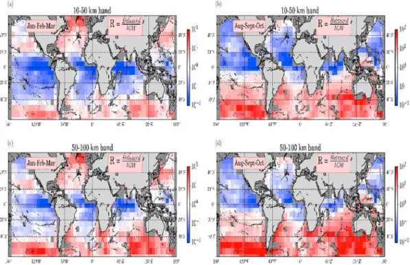
Figure 12. Global maps of the ratio R (see below) for kinetic energy at the ocean surface (estimated from a numerical
simulation): Top panels stand for submesoscale range (10–50 km); bottom panels stand for mesoscale range (50–100 km). Left panels are for January to March (winter in the Northern Hemisphere and summer in the Southern Hemisphere), and right panels are for August to September (summer in the Northern Hemisphere and winter in the Southern Hemisphere). For a given range of spatial scales, the variance above the dispersion relation curve for internal gravity waves (IGWs) corresponding to the highest baroclinic mode has been associated with IGWs and the one below this curve associated with balanced motions (BMs). R is the ratio between the variance associated with BMs and that associated with IGWs:R = BMvariance
IGWvariance. So for a given spatial-scale band, R> 1means that the variability of the flow is explained by BMs, and R< 1means that the variability of the flow is explained by IGWs. These panels emphasize the strong seasonality of the partition of kinetic energy into IGWs and BMs for scales smaller than 100 km and the strong regional diversity and differences between Northern and Southern Hemispheres (from Torres et al., 2018).
with BMs and has energy continuously spread out in the𝜔-k space, suggesting strong energy exchanges through nonlinear interactions (Figure 11, panel ii).
Qiu et al. (2018) and Torres et al. (2018) defined a criterion to discriminate BMs and IGWs for two scale ranges (10–50 and 50–100 km). Their criterion R makes use of a𝜔-k spectrum (see caption of Figure 12 for the definition of R). From the definition of R, BMs dominate for R > 1 and IGWs for R < 1. Based on 12,000𝜔-k spectra that cover the global ocean, their results highlight that IGWs dominate BMs in many regions (region in blue in Figure 12). Results emphasize not only a strong seasonality (with BMs dominating in winter and IGWs in summer) but also a strong regional variability. These two studies further revealed that, in summer, the IGW impacts on SSH lead to a significant slope discontinuity on the SSH wavenumber spectrum, at scales smaller than 100 km, a discontinuity not observed on the KE spectrum. On the other hand, IGWs were found to have no impact on sea surface temperature (SST) and Sea Surface Salinity (SSS). These very different signatures of IGWs on SSH, KE, SST, and SSS indicate that exploiting the synergy of using different satellite observations should help to discriminate IGWs and BMs in the global ocean (Torres et al., 2018). In that context, it is important to mention that, in addition to the SWOT mission, a future Wind and Current Mission (WaCM), still under development, aims to produce simultaneous observations of wind stress and surface oceanic currents at high resolution (Rodríguez et al., 2018). The strong potential of WaCM will be to observe not only surface currents but also the wind work (i.e., the dot product of the wind stress and surface currents) and therefore to identify the wind-driven near-inertial motions that have no signature in SSH (Gill et al., 1974).
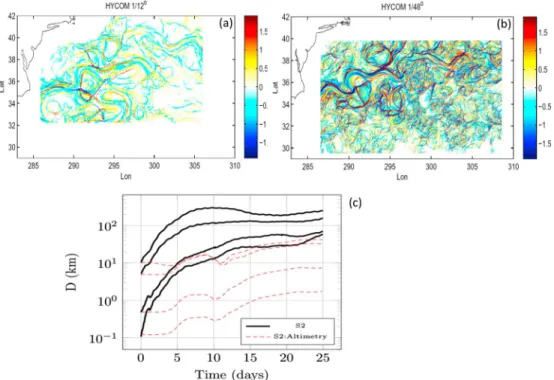
Figure 13. Finite Size Lyapunov Exponent from a simulation without (a) and with submesoscales (b). The color panels
indicate Finite Size Lyapunov Exponent in day−1. Blue colors show inflowing/stable trajectories from forward in time, and red colors show outflowing/unstable trajectories from backward in time particle advection. (from Haza et al., 2012, used with permission.) (c) Separation distance of a particle pair as a function of time, D(t), estimated in the Gulf of Mexico using (1) high-resolution data from 300 drifters (black curves) and (2) low-resolution AVISO sea surface height data (red). Dispersion is found to be 10–100 times larger when high-resolution data are used (from Poje et al., 2014, used with permission.).
6. Impact of Ocean Mesoscale/Submesoscale Turbulence on the Earth Climate
BMs (including mesoscale and submesoscale motions) are now known to have a strong impact on the large-scale ocean circulation, the ocean biology, and on the coupled ocean-atmosphere system, through the vertical and horizontal fluxes of any quantities. Recent studies, based on satellite altimeter products com-bined with in situ observations and on results from numerical simulations within large domains at high resolution, have highlighted the ocean turbulence contribution to the transport of heat, mass, chemical constituents of seawater, and air-sea interactions. In this section, we discuss some examples related to the impacts of this turbulence (that includes submesoscale fronts) on ocean dynamics and air-sea interactions. Impacts on ocean biology and carbon storage are discussed in recent review papers such as Lévy et al. (2012), Mahadevan (2016), and McGillicuddy Jr (2016).6.1. Stirring and Mixing Properties
The stretching (or strain) field and the Lagrangian accelerations associated with geostrophic eddies deter-mine the properties of the dispersion of tracers and particles (Hua & Klein, 1998; Lapeyre et al., 1999). In GT, the k−3KE spectrum slope implies that only by the largest eddies are responsible of the stretching of small-scale filaments. The tracer fluxes from large to small scales are associated with “nonlocal” scale inter-actions as the large scales control the small scales (Scott, 2006). However, when the KE spectrum slope is in k−2, such as when energetic submesosale fronts/eddies are present, filament dynamics are controlled by all eddies (including submesoscale eddies). Such interactions are called “local” since small-scale filaments can be produced by the smallest eddies (Scott, 2006). In that case the dispersion properties are much differ-ent from those driven by GT (Foussard et al., 2017; Özgökmen et al., 2012; Scott, 2006). Differences between local and nonlocal properties are well highlighted by maps of Finite Size Lyapunov Exponents as displayed in Figures 13a and 13b (from Haza et al., 2012). When submesoscale fronts/eddies are taken into account, FSLE are characterized by scales much smaller and magnitudes much larger (i.e., more intense stirring) than when submesoscale fronts/eddies are not taken into account.
Figure 14. Global patterns of vertical heat transport (estimated from a numerical simulation) explained by
submesoscales (<50 km) in winter (January–March for the Northern Hemisphere and July–September for the Southern Hemisphere). Values are spatially smoothed over 3◦×3◦square boxes; positive values indicate upward. In most area of midlatitudes, vertical heat transport at submesoscales is∼20–200 W/m2and is systematically upward (adapted from Su et al., 2018, used with permission).
Figure 13c (from Poje et al., 2014) issued from the analysis of high-resolution observations from surface drifters (that take into account submesoscale fronts and eddies) and SSH observations (that do not resolve submesoscale fronts and eddies) further quantifies the contribution of submesoscale fronts/eddies on the particle dispersion: particle dispersion is larger by at least 1 order of magnitude when estimated from high-resolution observations that include submesoscales (black curves in Figure 13c) than with observations that do not include submesoscales (such as those from AVISO SSH; see the red dashed curves in Figure 13c).
6.2. Horizontal Heat Transport
Hausmann and Czaja (2012) analyzed the relationship between satellite microwave SST and altimeter SSH observations. In regions of large SSH variability, SST and SSH mesoscale anomalies are nearly in-phase, involving intense warm-top anticyclones and cold-top cyclones. In quieter regions, weaker SST signa-tures are almost in quadrature with eddy SSH. These authors found that eddies flux heat poleward in the mixed-layer over a broad range of oceanic regimes. Magnitude of this heat transport, particularly significant in the Antarctic Circumpolar Current region, attains ∼ 0.2 PW, a value similar to that found by other studies using different observations, in particular the ARGO float data set (see Dong et al., 2014; Qiu & Chen, 2005) and studies using numerical simulations (Lévy et al., 2010). However, Hausmann and Czaja (Hausmann & Czaja, 2012) found that the poleward (equatorward) propagation of warm anticyclones (cold cyclones) pro-duces a much weaker poleward heat transport in the mixed layer than the horizontal fluxes resulting from the westward phase shift between SST and SSH fluctuations. In other words, the meridional heat transport is not so much due to individual eddies transporting temperature anomalies, but it is principally due to hor-izontal heat fluxes resulting from the stirring of temperature anomalies by mesoscale eddies. This finding points to the importance of the phase shift between SSH and SST mesoscale anomalies for the estimation of the meridional heat fluxes. Lévy et al. (2010) further revealed that taking into account the impact of the sub-mesoscale structures, in addition to that of sub-mesoscale eddies, does not lead to a systematic increase of the total meridional heat transport. Rather, impacts of submesoscale structures lead to significantly decrease this transport in some regions and increase it in others (see their Figure 12).
6.3. Vertical Heat Transport
Submesoscale frontal dynamics are known to be characterized by O(1) Rossby number and to capture most of the vertical velocity field in the upper ocean (Klein & Lapeyre, 2009; McWilliams, 2016; Mensa et al., 2013; Sasaki et al., 2014; Thompson et al., 2016). One consequence, revealed by Hakim et al. (2002) and confirmed by Lapeyre and Klein (2006) and McWilliams et al. (2009; see also Fox-Kemper et al., 2008, 2011), is that these submesoscale fronts are associated with positive vertical heat fluxes, that is, upgradient (from deep cold waters to surface warm waters) and not downgradient. This adiabatic property has been highlighted in a recent paper by Su et al. (2018) using an OGCM at unprecedented high spatial resolution (2 km in the horizontal and 90 vertical levels). Results indicate that upper ocean submesoscale turbulence produces a systematically upward heat transport that is 5 to 10 times larger than the vertical heat transport explained by mesoscale eddies! Wintertime magnitudes of these submesoscale heat fluxes are up to 200 W/m2for
mid-Figure 15. Vertical distribution of the modeled (left column) zonal velocity (cm/s) and (right column) eddy kinetic
energy (cm2/s2) along 55◦W for the (1/50)◦, (1/25)◦, and (1/12)◦numerical simulations (from Chassignet & Xu, 2017, © American Meteorological Society. Used with permission).
latitudes (when averaged over 3 months and in boxes of 300-km size; see Figure 14). These vertical heat fluxes warm the sea surface by up to 0.3◦C annually and produce an upward annual-mean air-sea heat flux anomaly of 4–10 W/m2at midlatitudes (Su et al., 2018). Such results indicate that submesoscale BMs
asso-ciated with submesoscale frontal structures are critical to the vertical transport of heat between the ocean interior and the atmosphere and are thus a key component of the Earth's climate. Noting that submesoscale fronts are preconditioned by mesoscale eddies, the results from Su et al. (2018) further highlight the impacts of the ocean-scale interactions on the Earth Climate.
6.4. Impact of Submesoscale Fronts on the Large-Scale Ocean Circulation
The impact of submesoscale frontal physics on the large-scale ocean circulation has been examined by Lévy et al. (2010) and Chassignet and Xu (2017). To test this impact, these authors used several numerical mod-els at a basin scale, each one with a different spatial resolution. After a reasonable spin-up period (10–20 years), the large-scale ocean circulation and the mean structure of the ventilated thermocline strongly differ when the resolution increased from 10 to 2 km (which highlights the impact of submesoscales). Changes involve the emergence of a denser and more energetic eddy population at the 2-km resolution, occupy-ing most of the basin and sustained by submesoscale physics. Takoccupy-ing into account submesoscale dynamics leads to “regional” and “remote” effects. Regional effects occur through the inverse KE cascade that strongly intensifies zonal jets such as in the Gulf Stream region. This intensification subsequently leads to isopycnals steepening (through the thermal wind balance), which significantly counterbalances and locally overcomes the eddy-driven heat transport that tends to flatten isopycnals (Lévy et al., 2010). Chassignet and Xu (2017) further note that, when the spatial resolution is increased, the representation of the Gulf Stream penetration and associated recirculating gyres changes from unrealistic to realistic (in terms of comparison with obser-vations) and that the penetration into the deep ocean drastically increases (see Figure 15). Remote effects occur through the resulting general equilibration of the main thermocline that shifts zonal jets at midlati-tudes southward by a few degrees, significantly altering the shape and position of the gyres. Consequence is that the deep convection in high latitudes is reduced, leading to a significant modification of the merid-ional overturning circulation. Thus, results from Lévy et al. (2010) and Chassignet and Xu (2017) emphasize
that the impact of submesoscale fronts on the mean circulation and mean transport at a basin scale cannot be ignored anymore. There is a need to repeat these two numerical experiments in larger domains with an even higher spatial resolution (J. Callies, personal communication), in particular on the vertical, using the coming exascale computers.
6.5. Air-Sea Interaction
Chelton et al. (2004) discovered a remarkably strong positive correlation between surface winds and SST at mesoscale (i.e., 100–300 km) using a combination of radar scatterometers and SST observations. As shown later by Frenger et al. (2013), mesoscale eddies are characterized by a positive correlation between SST, SSH, cloudiness, and precipitation rate. Similar correlations were found between air-sea heat fluxes and SST (Bôas et al., 2015; Byrne et al., 2015; Ma et al., 2015). An arising question concerns the impact of OMT at the scale of the atmospheric storm track (i.e., O(5,000–10,000 km)). Ma et al. (2015) and Foussard et al. (2019) showed that increased air-sea heat fluxes at the ocean surface, due to oceanic eddies, could lead to a nonlocal response associated with a modification of the atmospheric circulation far from the oceanic eddying region. In parallel, using numerical models with spatial resolution accounting for scales as small as 50 km, Minobe et al. (2008) showed that local SST fronts in the Gulf Stream could impact the entire troposphere. These authors found a conspicuous signal in their atmospheric general circulation model, indicating a wind con-vergence over the warm flank of the oceanic front up to 12 km in altitude (i.e., close to the tropopause). One important characteristic is that the wind convergence was found to be proportional to the SST Laplacian (a second-order derivative that involves small scales). This sensitivity to small scales explains why past numer-ical models, with lower resolution, were unable to represent such dynamics (Bryan et al., 2010). Since then, numerous studies with higher spatial resolution have highlighted the importance of such SST gradients, with scales down to the submesoscales, for the tropospheric storm tracks (Deremble et al., 2012; Foussard et al., 2019; Nakamura et al., 2008). These results have led to a renewed interest in understanding the role played by SST anomalies at scales down to 5–10 km in atmosphere dynamics.
Although the ocean current magnitude is much smaller than the atmospheric wind speed, a large number of numerical studies, at least in the last two decades, have shown that oceanic currents at mesoscales and submesoscales can also significantly impact the wind stress. In terms of ocean dynamics, the resulting effects on the wind work lead to a net KE transfer from the ocean to the atmosphere. This transfer corresponds to a decay of almost 30% of the ocean KE at mesoscale at midlatitudes (Eden & Dietze, 2009) and less than 20% for oceanic submesoscales (Renault et al., 2018). In terms of atmospheric dynamics, the wind stress curl and divergence resulting from the ocean current impacts should affect the vertical velocity in the atmosphere. A recent in situ experiment has been carried out in the Gulf of Mexico using a Doppler Scatterometer to observe simultaneously the surface currents and wind stress at very high resolution (∼2.5 km). The results reveal and confirm the strong correlation between the wind stress curl and the relative vorticity associated with oceanic submesoscales (E. Rodriguez, personal communication, November, 2018). Magnitude of the wind stress curl is such that the wind divergence in the atmosphere is 1 order of magnitude larger than found by Minobe et al. (2008).
These results further confirm that oceanic mesoscale eddies and submesoscales structures can significantly impact the atmospheric boundary layer and the whole troposphere. There is still some work to do to further quantify these impacts and the consequences on the atmospheric storm tracks.
7. Discussion and Conclusion
Analysis of altimeter observations collected in the last 25 years and results obtained from OGCMs with high spatial resolution emphasize that all the oceans are fully turbulent, involving a broad range of scales from at least 2 km to 5,000 km. All these scales are now known to strongly interact, leading to signifi-cant energy exchanges between scales, in particular in the upper ocean. Resulting ocean-scale interactions impact the Earth climate in counterintuitive ways. For instance, the smallest scales render mesoscale eddies more coherent with a longer lifetime and can also trigger significant upgradient and not downgradient ver-tical fluxes of any quantity. A better understanding of the IGWs impacts may lead to a more complex vision depending on how much they interact with BMs. Overall, results highlight that the oceanic fluid is much less diabatic and much more inertial than thought 25 years ago (i.e., again with fluxes much less controlled by diffusivity or viscosity and more by nonlinear interactions that lead to reversible upgradient and down-gradient fluxes). Numerous studies now emphasize that these ocean-scale interactions are crucial for the
BMs and internal gravity waves have different impacts in terms of fluxes on the KE budget, which points to the need to discriminate them from observations. In that respect, future wide-swath altimeter missions, such as the SWOT mission (Fu & Ferrari, 2008), will be critical to make major advances. These observations are the only ones capable to diagnose correctly BMs down to scales of 30–50 km. However, these future SSH observations will have to be combined with existing satellite observations as well as with those from missions under development to retrieve other IGWs. The latter missions include WaCM (Rodríguez et al., 2018), already mentioned, that will observe simultaneously the wind stress and oceanic currents at very high resolution and therefore give access to near-inertial waves and smaller IGWs. They also include other missions such as the Surface KInematic Monitoring mission (Ardhuin et al., 2018) and the Wavemill mission (Martin et al., 2016) aiming to observe surface currents with high resolution. An optimal strategy to better capture the subtleties of ocean turbulence would be to exploit the synergy of analyzing all these satellite observations in combination with in situ data on a global scale, such as the ones collected by surface drifters (Lumpkin et al., 2017) and ARGO floats (Le Traon, 2013) deployed in all oceans.
The importance, for the Earth climate, of fully taking into account the ocean-scale interactions is further emphasized by recent geophysical studies on the Earth atmosphere and oceans. The Earth atmosphere involves cyclones and anticyclones (although with larger scales than in the oceans) that strongly interact the so-called atmospheric storm tracks. However, if geophysical turbulence refers to an inverse KE cascade over a broad inertial range (defined as the scale range between the eddy source scale and the scale of the most energetic eddies), the atmosphere is found much less turbulent than the oceans (Jansen & Ferrari, 2012). The atmosphere is indeed characterized by an inverse KE cascade over a very small inertial range compared to the oceans (Merlis & Schneider, 2009; Schneider & Walker, 2006). Scales of the atmospheric cyclones and anticyclones are close to their source scales (scales of the baroclinic instability). On the other hand, as pointed out several times in this paper, the OMT is characterized by an inverse KE cascade over a broad inertial range (Hua & Haidvogel, 1986; Hua et al., 1998). The consequence, as discussed by Jansen and Ferrari (2012), is that the atmospheric response to external forcings is much faster and much less iner-tial than the ocean response, which should impact the dynamics of the coupled ocean-atmosphere system. These differences between the ocean and atmosphere turbulent properties emphasize the importance of the future developments on ocean-scale interactions for studies of climate and climate change (Jansen & Ferrari, 2012).
References
Alford, M. H., MacKinnon, J. A., Simmons, H. L., & Nash, J. D. (2016). Near-inertial internal gravity waves in the ocean. Annual Review of
Marine Science, 8, 95–123.
Arbic, B. K., Polzin, K. L., Scott, R. B., Richman, J. G., & Shriver, J. F. (2013). On eddy viscosity, energy cascades, and the horizontal resolution of gridded satellite altimeter products. Journal of Physical Oceanography, 43(2), 283–300.
Arbic, B. K., Scott, R. B., Flierl, G. R., Morten, A. J., Richman, J. G., & Shriver, J. F. (2012). Nonlinear cascades of surface oceanic geostrophic kinetic energy in the frequency domain. Journal of Physical Oceanography, 42(9), 1577–1600.
Ardhuin, F., Aksenov, Y., Benetazzo, A., Bertino, L., Brandt, P., Caube, A. P., et al. (2018). Measuring currents, ice drift, and waves from space: The sea surface kinematics multiscale monitoring (SKIM) concept. Ocean Science, 14, 337–354.
Aref, H. (1984). Stirring by chaotic advection. Journal of Fluid Mechanics, 143, 1–21.
Barkan, R., Winters, K. B., & McWilliams, J. C. (2017). Stimulated imbalance and the enhancement of eddy kinetic energy dissipation by internal waves. Journal of Physical Oceanography, 47(1), 181–198.
Blumen, W. (1978). Uniform potential vorticity flow: Part I. Theory of wave interactions and two-dimensional turbulence. Journal of the
Atmospheric Sciences, 35(5), 774–783.
Acknowledgments
We dedicate this study to our colleague and friend Bach Lien Hua who was the first woman to give a Lorenz Conference (in 2006) and who made so many significant and insightful contributions to the understanding of oceanic turbulence. We thank the two reviewers for their constructive comments and in particular Eric Chassignet for his advices during the revision process. We also thank Jinbo Wang for his insightful comments. This study was carried out at the Jet Propulsion Laboratory, California Institute of Technology, under contract with the National Aeronautics and Space Administration (NASA), at the Laboratoire de Météorologie Dynamique and at the Courant Institute. P. K. is supported by a NASA Senior Fellowship and the SWOT mission. G. L. is supported by the CNES-SWOT mission. L. S. is a JPL JVSRP affiliate and is supported by a joint CNES-Région Bretagne doctoral grant. B. Q. and L. L. F. acknowledge support from the NASA SWOT mission (NNX16AH66G). H. T. and D.M. are supported by NASA Physical Oceanography (PO) and Modeling, Analysis, and Prediction (MAP) Programs. Z. S. has been supported by NASA NPP postdoc fellowship and NASA grant NNX15AG42G. This work is partly funded by CNES (OSTST-OSIW grant). Data used in this paper can be found in the NASA website (https://science.jpl.nasa.gov/ projects/ECCO-IcES/).