Subjective and objective rating of intelligibility of speech recordings

(1)

Publisher’s version / Version de l'éditeur:

Vous avez des questions? Nous pouvons vous aider. Pour communiquer directement avec un auteur, consultez la première page de la revue dans laquelle son article a été publié afin de trouver ses coordonnées. Si vous n’arrivez pas à les repérer, communiquez avec nous à PublicationsArchive-ArchivesPublications@nrc-cnrc.gc.ca.

Questions? Contact the NRC Publications Archive team at

PublicationsArchive-ArchivesPublications@nrc-cnrc.gc.ca. If you wish to email the authors directly, please see the first page of the publication for their contact information.

https://publications-cnrc.canada.ca/fra/droits

L’accès à ce site Web et l’utilisation de son contenu sont assujettis aux conditions présentées dans le site

LISEZ CES CONDITIONS ATTENTIVEMENT AVANT D’UTILISER CE SITE WEB.

123rd Audio Engineering Society Convention [Proceedings], pp. 1-12, 2007-10-05

READ THESE TERMS AND CONDITIONS CAREFULLY BEFORE USING THIS WEBSITE. https://nrc-publications.canada.ca/eng/copyright

NRC Publications Archive Record / Notice des Archives des publications du CNRC : https://nrc-publications.canada.ca/eng/view/object/?id=d8d3b0f9-937a-430b-9174-29085941dcec https://publications-cnrc.canada.ca/fra/voir/objet/?id=d8d3b0f9-937a-430b-9174-29085941dcec

NRC Publications Archive

Archives des publications du CNRC

This publication could be one of several versions: author’s original, accepted manuscript or the publisher’s version. / La version de cette publication peut être l’une des suivantes : la version prépublication de l’auteur, la version acceptée du manuscrit ou la version de l’éditeur.

Access and use of this website and the material on it are subject to the Terms and Conditions set forth at

Subjective and objective rating of intelligibility of speech recordings

(2)

S u b j e c t i v e a n d o b j e c t i v e r a t i n g o f

i n t e l l i g i b i l i t y o f s p e e c h r e c o r d i n g s

N R C C - 5 0 0 8 7

G o v e r , B . N . ; B r a d l e y , J . S .

A version of this document is published in / Une version de ce document se trouve dans: 123rd Audio Engineering Society Convention, New York, N.Y., Oct. 5-8, 2007, pp. 1-12

The material in this document is covered by the provisions of the Copyright Act, by Canadian laws, policies, regulations and international agreements. Such provisions serve to identify the information source and, in specific instances, to prohibit reproduction of materials without written permission. For more information visit http://laws.justice.gc.ca/en/showtdm/cs/C-42

Les renseignements dans ce document sont protégés par la Loi sur le droit d'auteur, par les lois, les politiques et les règlements du Canada et des accords internationaux. Ces dispositions permettent d'identifier la source de l'information et, dans certains cas, d'interdire la copie de documents sans permission écrite. Pour obtenir de plus amples renseignements : http://lois.justice.gc.ca/fr/showtdm/cs/C-42

(3)

Audio Engineering Society

Convention Paper

Presented at the 123rd Convention 2007 October 5–8 New York, NY, USA

The papers at this Convention have been selected on the basis of a submitted abstract and extended precis that have been peer reviewed by at least two qualified anonymous reviewers. This convention paper has been reproduced from the author's advance manuscript, without editing, corrections, or consideration by the Review Board. The AES takes no responsibility for the contents. Additional papers may be obtained by sending request and remittance to Audio Engineering Society, 60 East 42nd Street, New York, New York 10165-2520, USA; also see www.aes.org. All rights reserved. Reproduction of this paper, or any portion thereof, is not permitted without direct permission from the Journal of the Audio Engineering Society.

Subjective and objective rating of

intelligibility of speech recordings

Bradford N. Gover and John S. Bradley

Institute for Research in Construction, National Research Council, Ottawa, Ontario K1A 0R6, Canada brad.gover@nrc-cnrc.gc.ca

ABSTRACT

Recordings of test speech and an STIPA modulated noise stimulus were made with several microphone systems placed in various locations in a range of controlled test spaces. The intelligibility of the test speech recordings was determined by a subjective listening test, revealing the extent of differences among the recording systems and locations. Also, STIPA was determined for each physical arrangement, and compared with the intelligibility test scores. The correlation between STIPA and the intelligibility scores was not found to be high in all situations. A computer program was written to determine STIPA in accordance with IEC 60268-16. The result was found to be highly sensitive to the method of determining the modulation transfer function at each modulation frequency, yielding the most accurate result when normalizing by the pre-measured properties of the specific stimulus used.

1. INTRODUCTION

Speech recordings are made for a variety of reasons, including audio transcripts, archiving, broadcast, or transmission. In some cases, the people speaking are attempting to speak directly into a microphone, but in other instances, they may be at a distance from one, or even unaware that a recording is taking place. In any situation, a basic intention of such a recording is that the speech be intelligible. Under adverse conditions, such as reverberation, high noise, or distant microphone location, this can be quite challenging.

For a given room, having its own reverberant and characteristic noise response, a more or less intelligible speech recording may result from using

different microphone systems or placements. It is of interest to understand the magnitude of the differences in performance, to allow for optimal device selection and placement.

It is also of interest to be able to predict or rank-order the performance of recording systems using an objective measure. The STIPA measure defined in IEC 60268-16 [1] is potentially well suited for this purpose. STIPA has been shown to be well correlated with the original STI measure under a range of conditions [2], however it is not without its problems [3]. In theory, STIPA could be measured for various recording system placements, and the subjective intelligibility predicted.

This paper presents some results of physical measurements and subjective listening tests for speech recordings made under controlled conditions.

(4)

2. PROCEDURES AND EQUIPMENT

For each of the four test spaces, one loudspeaker

The loudspeaker used was an NTI TalkBox [4],

The test sentences were in English,

phonetically-Device Channels Directionality Additional description

Test speech was recorded with a variety of microphone systems in four test spaces, spanning a wide range of acoustical conditions. The intelligibility of the recordings was determined from a subjective listening test, and STIPA was also determined. Section 2 below describes the procedures, facilities, and equipment used. Section 3 describes the listening test and its results. Section 4 presents the STIPA results; Section 5 some potentially important issues related to its calculation. Section 6 offers some conclusions.

(talker) position and three microphone (recording) positions were chosen. The test speech and STIPA modulated noise stimulus were played at a fixed level over a small loudspeaker and recorded with a number of microphone systems, located in turn at each recording position. The recording devices are described in Sec. 2.1, and the test spaces are described in Sec. 2.2.

which is intended for speech intelligibility testing. It consists of a single 12 cm driver in a small box (approximately 15 x 15 x 15 cm). The TalkBox includes a CompactFlash card playback system that plays digital (.wav) files at a fixed level, equalized to be flat on axis. The test signals and sentences reported in this paper were played at a fixed level in each test space: 50 dBA (at 1 m, free field) for three of the test spaces, and 60 dBA (at 1 m, free field) in the other. Refer to Sec. 2.2 for details. The level and equalization were verified in an anechoic chamber.

balanced, and of low predictability [5]. For each

configuration of each microphone system in each recording position, 5 unique test sentences were recorded.

2.1. Recording Devices

In total, seven different microphone systems (devices) were used. Brief descriptions are presented in Table 1. The term “device” is used to refer to not only the microphone(s), but also all associated signal processing and amplification. The naming convention used was to label each D1, D2, D3, and so on. Devices D1, D2, D3 are commercial devices, all using omnidirectional microphone elements. Device D4 refers to a pair of omnidirectional laboratory microphones (B&K type 4190), and a fixed-gain preamplifier (GRAS 12AA). No additional processing was involved. Devices D5 and D7 (the latter used only in one room) were cardioid electret cartridges with fixed-gain amplification. Device 6 was a 6-element curvilinear array with a directional gain of 7 dB from 400-4000 Hz, and fixed-gain amplification.

The three commercial devices (D1, D2, and D3) were used in some locations with multiple settings (e.g., different levels of compression). In the naming convention, these were referred to as different device configurations, and C1, C2, or C3 was appended to the device name.

The microphone recording locations within each room were named M1, M2, and M3. When placing a 2-channel device, the microphones were placed 30 cm apart, with one at the nominal position (to allow direct comparison with the 1-channel devices). The only 2-channel recordings where the microphones were not 30 cm apart were for device D2 in configuration C2, where they were 0.5 cm apart.

D1 1 Omni Equalization, compression

D2 2 Omni CODEC

D3 2 Omni Recorder using perceptual coding

D4 2 Omni Pair of laboratory microphones and preamps

D5 1 Cardioid Cardioid electret

D6 1 Array 6-element curvilinear array

D7 1 Cardioid Cardioid electret

(5)

Gover and Bradley Intelligibility of Speech Recordings

In the following, naming codes DiCjMk (i,j,k = 1,2,3) appear, used to refer to specific measurement cases for a particular device, configuration, and placement. For example, to refer to device D1 in configuration C2 in microphone location M3, the code “D1C2M3” is used.

2.2. Test Spaces

As stated above, the four test spaces used for the recording and measurements were selected to have widely different acoustical properties. The spaces were named C, K, R, and T, and are described in the following subsections.

2.2.1. Test Space C

Test Space C was the most reverberant of the four spaces. It was a concrete reverberation chamber,

measuring 8.3 x 5.1 x 3.5 m, into which were brought several pieces of absorptive foam, to control reverberation. A plan drawing of the room is shown in Fig. 1(a). Also indicated in the figure are the locations of the test loudspeaker (S) and microphone devices (M1, M2, and M3). The reverberation time (measured with the NTI TalkBox loudspeaker) in each octave band is shown in Fig. 1(b). RT was about 1.5 s up to 1 kHz, dropping to 0.6 s at 8 kHz. For the testing, a 30 s recording of mechanical system noise was played (looped continuously) into the room via a pair of loudspeakers located in the far corners of the room (i.e., away from the test loudspeaker and microphone locations). The spectrum of the noise measured in the room is shown in Fig. 1(c), and it had an overall level of 46.1 dBA. The test speech and STIPA signal were played at a fixed level of 50 dBA at 1 m in a free field.

(b)

(a)

(c)

Figure 1 Test Space C: (a) plan view indicating test loudspeaker position (S), and microphone device locations (M1, M2, and M3), (b) octave-band reverberation times, and (c) background noise spectrum (overall level 46.1 dBA).

AES 123rd Convention, New York, NY, USA, 2007 October 5–8 Page 3 of 12

(6)

2.2.2. Test Space K

Test Space K was a 6.7 x 4.1 x 2.8 m carpeted listening room, fitted with a table and chairs. A plan drawing is shown in Fig. 2(a), indicating the locations of the test loudspeaker (S) and the microphone devices (M1, M2, and M3). The reverberation time (measured with the NTI TalkBox loudspeaker) in each octave band is shown in Fig. 2(b). RT was less than 0.6 s at all frequencies,

having a value of 0.4 s at 1 kHz, and dropping to nearly 0.2 s at 8 kHz. For the testing, a 60 s recording of residential dishwasher noise (looped continuously) was played into the room via a single loudspeaker located next to the table behind position S. The spectrum of the noise measured in the room is shown in Fig. 2(c), and it had an overall level of 49.9 dBA. The test speech and STIPA signal were played at a fixed level of 50 dBA at 1 m in a free field.

(b)

(a)

(c)

Figure 2 Test Space K: (a) plan view indicating test loudspeaker position (S), and microphone device locations (M1, M2, and M3), (b) octave-band reverberation times, and (c) background noise spectrum (overall level 49.9 dBA).

(7)

2.2.3. Test Space R

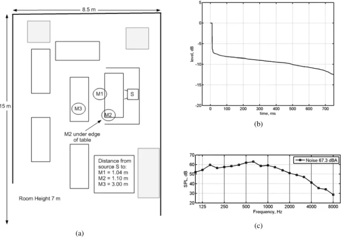
Test Space R was a very large room containing several tables and chairs. The dimensions of the room were 15 x 8.5 x 7 m. A plan drawing of part of the space is shown in Fig. 3(a), indicating the locations of the test loudspeaker (S), and the recording microphones (M1, M2, and M3). The reverberation time in this room was very difficult to measure due to the fact that the early arriving sound was due to a small number of strong discrete reflections, and the late, reverberant field was masked by the room noise. The reverse-integrated

“Schroeder” decay curve shown in Fig. 3(b) is therefore stepwise over the first 10 dB or so, and then “in the noise”. Acoustically, it behaves as a nearly anechoic, noisy space. For the testing, a 45 s segment of noise recorded in a busy restaurant was played into the room (looped continuously) via a four loudspeakers located away from the testing area. The spectrum of the noise measured in the room is shown in Fig. 3(c), and it had an overall level of 67.3 dBA. The test speech and STIPA signal were played into this test space at a fixed level of 60 dBA at 1 m in a free field.

(b)

(a)

(c)

Figure 3 Test Space R: (a) plan view indicating test loudspeaker position (S), and microphone device locations (M1, M2, and M3), (b) broadband level decay curve, and (c) background noise spectrum (overall level 49.9 dBA).

(8)

2.2.4. Test Space T

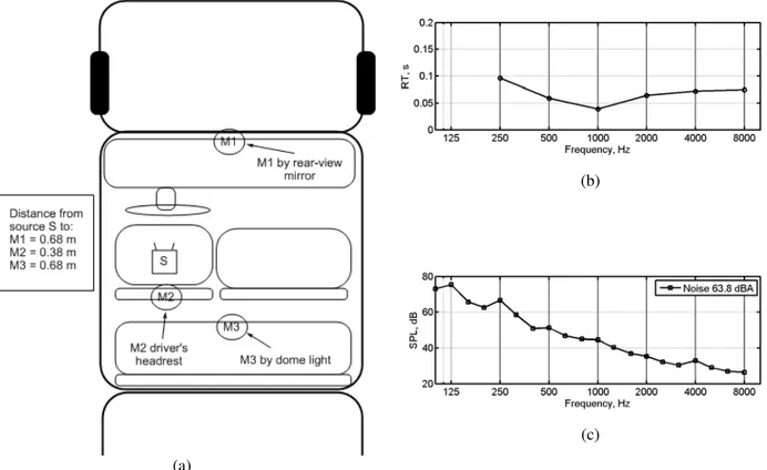
Test Space T was the passenger cabin of a full-size pickup truck (Chevrolet Cheyenne 2500). This space was smaller and less reverberant than the others used. A plan view is shown in Fig. 4(a), indicating the loudspeaker position (S) at the driver’s head location, and microphone locations (M1, M2, and M3). The reverberation time (measured with the NTI TalkBox loudspeaker) in each octave band is shown in Fig. 4(b). RT was less than 0.1 s at all frequencies. For

the testing, the truck was stationary and not running, but a 6 s segment of noise recorded while it had been driving at 50 km/h was played (looped continuously) via two loudspeakers (one located on the bench seat behind S, the other on the floor of the passenger side), neither pointed at the measurement area. The measured spectrum of the noise is shown in Fig. 4(c), and it had an overall level of 63.8 dBA. The test speech and STIPA signal were played at a fixed level of 50 dBA at 1 m in a free field.

(b)

(a)

(c)

Figure 4 Test Space T: (a) plan view indicating test loudspeaker position (S), and microphone device locations (M1, M2, and M3), (b) octave-band reverberation times, and (c) background noise spectrum (overall level 63.8 dBA).

(9)

3. LISTENING TEST

In total, there were 83 sets of recordings made, 44 of which were 2-channel. These resulted from combinations of device Di in configuration Cj in microphone positions Mk, for most (but not all) possible combinations. The 2-channel recordings were treated as 1-channel by considering only one channel. Counting the 1-channel and 2-channel recordings separately resulted in 83 + 44 = 127 unique test conditions. For each of the 127 test conditions, 5 test sentences were recorded, for a total of 635 test sentences. One-quarter of these sentences was played for each of 40 listening test subjects, distributed so that by the end of testing, each test sentence was heard and rated by 10 subjects. None of the subjects had significant hearing loss and all spoke English as a first language. The testing protocol was approved by the NRC Research Ethics Board (NRC O-REB Protocol 2006-47).

3.1. Description

The listening test subjects listened over headphones (Sennheiser HD 280) at a fixed, comfortable level (that they selected). One at a time, the recorded sentences were played. The subjects were instructed that after each sentence was played they should repeat (speak out loud) the words they were able to understand. The test operator scored the word intelligibility by noting those words correctly identified. The scores were normalized to indicate the fraction of words correctly identified, ranging from 0 (none) to 1 (all).

3.2. Results

The word intelligibility scores from 10 subjects for all 5 test sentences for a given microphone device case (i.e., device Di, device configuration Cj, location Mk) were averaged. The mean score for a particular device placement is therefore the average of 50 subjective responses.

The results for all test conditions are shown in Fig. 5. The black bars are for the 1-channel (mono) recordings, and the light grey bars are for the 2-channel (stereo) recordings. An asterisk (*) to the left of a light grey bar (between the DiCjMk code and the bars themselves) indicates that the difference in score between the 1-channel and the 2-1-channel recording is statistically significant (p < 0.05). The absence of an asterisk next to a light grey bar indicates that the difference between the 1-channel and 2-channel scores is not significant.

Admittedly, Fig. 5 is dense with information, but close inspection indicates outcomes that may be useful to better understand the particular devices tested.

For example, the upper left plot shows the results from Test Space C. The top 11 measurement cases correspond to recordings made at microphone location M1. It can be seen that the most-intelligible recording was the 2-channel recording made with device D2 in configuration C1 (light grey bar D2C1M1), although D4C1M1 (pair of laboratory microphones) is not significantly different. The most intelligible 1-channel recording at this position was D6C1M1, for the directional array, although not significantly better than some of the 1-channel recordings from D2, D3, and D4. Device D5 (cardioid) resulted in the least-intelligible recordings: it was learned after testing that the microphone itself was significantly noisy. Device D1 (the top three bars) performed best in configuration C1, compared to D1C2M1 and D1C3M1.

At recording position M3 in Test Space R, the most intelligible 1-channel recordings were from device D6, the directional array. This location was 3 m from the source in a very noisy space, yet the word intelligibility was 0.8 (80%), much higher than any other device tested.

In Test Space T, the intelligibility scores for the recordings at position M1 are in general higher than for positions M2 and M3, which is not surprising given that these latter two are actually behind the speaking position. However, the recordings from device D2 (both 1 and 2-channel) and device D5 (cardioid) at position M2 were highly intelligible.

Results such as these demonstrate that important differences among the devices exist, and can be identified.

A more general observation is that the 2-channel scores are almost always higher than the 1-channel scores. For some cases, the word intelligibility was more than 0.2 (20%) higher for the 2-channel scores, which is a substantial difference. Evidently, this is an effect of a “binaural advantage” of stereo versus mono. This could provide useful guidance for users of 2-channel recording systems, when making decisions as to microphone placement.

(10)

Figure 5 Mean word intelligibility score results from the subjective listening test, grouped by Test Space. The black bars are for 1-channel recording and playback, and the light grey bars are for 2-channel. An asterisk (*) at the left indicates a significant difference (p < 0.05) between the corresponding 1 and 2 channel scores. The absence

(11)

4. STIPA RESULTS

As stated previously, in addition to recording the test sentences, for each device placement a recording was made of an STIPA modulated noise test stimulus. These recordings were processed in MATLAB (see below, Section 5) and the STIPA value for each measurement case was determined. For the 2-channel devices, only 1 channel was processed.

The listening test word intelligibility scores are plotted versus STIPA in Fig. 6, for all 83 1-channel device configurations. The overall correlation between the subjective scores and STIPA was not high: the R2 value (coefficient of determination) was 0.35. Broken down

by Test Space, it can be seen that the correlation was worst for Test Space R (R2=0.21), where the intelligibility scores were on average lowest, and best for Test Space K (R2 = 0.71).

The poor overall relationship between the listening test scores and the STIPA values indicates that STIPA may not generally be suitable for predicting the intelligibility of the recorded speech material. At an STIPA value of 0.5, word intelligibility scores ranging from almost 0 to almost 1 were observed. Omitting the Test Space R results, however, the relationship between intelligibility score and STIPA was stronger, indicating that in some situations the relationship may be more useful.

Figure 6 Mean word intelligibility scores of recorded sentences versus STIPA, for all 83 1-channel test cases. The different symbols indicate the breakdown by Test Space (C, K, R, or T).

(12)

5. CALCULATION OF STIPA

The STIPA stimulus used in the measurements was supplied by NTI with the TalkBox loudspeaker. The intention was to play the recordings into a Norsonic 118 analyzer equipped with the STIPA analysis option. However, after the recordings were made, it was learned that the process would not work since the stimulus is incompatible with the analyzer – the NTI stimulus is modulated differently than described in the IEC 60268-16 standard (see below, and [4]). This led to the need to calculate STIPA in software, which was done in MATLAB. Some issues are detailed below.

STIPA is calculated from the modulation transfer function, evaluated at two modulation frequencies per octave band. The modulation transfer function is the ratio of the modulation index of a test stimulus to the corresponding modulation index of the output of a system, having the test stimulus as input.

The well-known expression for the amplitude modulation of a test stimulus at a single modulation frequency F is

]

[

1 cos(

2 )

0

m

Ft

I

=

+

π

, (1 )

where m is the modulation index, I is the signal intensity (proportional to square of signal amplitude), and I0 is

the mean intensity (dc value). The test stimulus is designed with full-depth modulation (m = 1) at each modulation frequency of interest.

The two-frequency version (used for STIPA) where each octave band is modulated at frequencies F1 and F2,

both with the same modulation index of m, is

[

1 cos(

2

₁

)

cos(

2

₂

)

0

+

π

+

π

+

φ

]

=

I

m

F

t

m

F

t

I

. (2 )

For a particular F1 and F2, the maximum possible value

of m depends on the relative phase shift φ. In the assignment of frequencies in the STIPA scheme described in Annex C of IEC 60268-16, F1 is always

harmonically related to F2 by F2 = 5F1. It turns out that m can be as large as 0.55 (for a phase shift of π/2, for

example). This is mentioned, but not explained, in IEC 20268-16.

Annex C of IEC 20268-16 is “Informative”, not “Normative”, however, so there is not actually any requirement to use the assignment of modulation frequencies laid out therein. This is taken advantage of

in the NTI stimulus used in this work, which does not follow the proscribed scheme in the lower frequency bands. Rather than using a combined 2-octave-wide band for the 125-250 Hz range, the NTI scheme modulates them separately. The 125 Hz band is modulated at 1.6 and 8 Hz, and the 250 Hz band at 1 and 5 Hz [4].

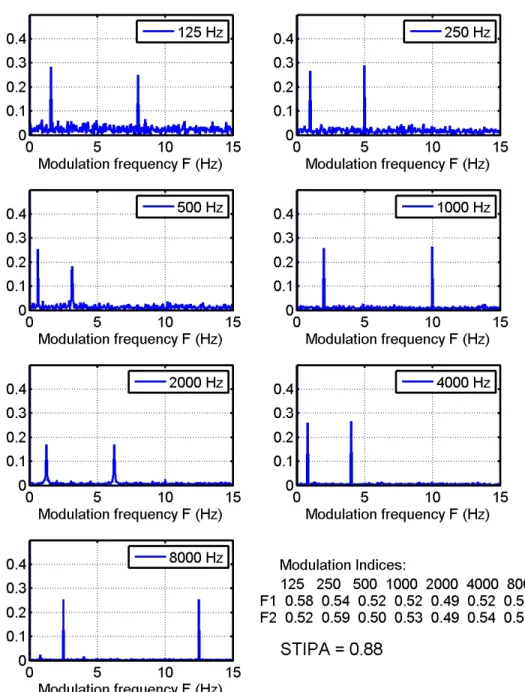
In developing a program to calculate STIPA, it was of course of interest to validate its performance. It should be possible to analyze the original stimulus itself and find modulation indices very close to 0.55, and therefore an STIPA value close to 1.0. This was not the case. Figure 7 shows the modulation spectrum of the stimulus used in the current measurements in each octave band from 125 to 8000 Hz. The spectra are normalized so that a single frequency modulation with a modulation index of m = 0.55 should appear as a narrow peak with height equal to 0.55/2 = 0.275. This is not precisely true for all peaks.

To calculate the modulation transfer function, and hence STIPA, from octave band modulation spectra such as those in Fig. 7 (or corresponding ones following transmission of the stimulus through a system under consideration), there is the need to determine the modulation index for each modulation frequency. Essentially, the amplitudes of the peaks at the modulation frequencies need to be determined. This raises the question of how. It seems reasonable to assume that the modulation of the noise stimulus is (or should be?) single-frequency, so it is tempting to determine the peak height (i.e., take the amplitude of the single FFT bin corresponding to the modulation frequency). This leads to errors when the modulation peak has breadth, as is seen, for example, in the 2000 Hz octave band. Reference [6] implies a one-third-octave filtering approach: doing so includes a lot of “noise” outside the single-frequency of interest. This can be mitigated somewhat, but not entirely, by narrowing the fractional octave bands under consideration. This was done herein.

As stated above, in calculating the modulation index from the stimulus itself (from the .wav file data), values of 0.55 were not found at all modulation frequencies. Refer to the values in Fig. 7. This is of course not too surprising since it is a modulated noise signal and there will be some variation due to the random nature of the noise.

(13)

Figure 7 Octave band modulation spectra for one 30 s segment of NTI STIPA test stimulus, and corresponding modulation indices. The resulting STIPA was 0.88.

However, repeated analyses of many segments of the stimulus, of varying lengths, were averaged, and the mean modulation indices did not converge to 0.55. The modulation indices shown in Fig. 7 were found for one 30 second segment, and led to an STIPA value of 0.88

when normalized by an “expected value” of 0.55 to obtain the modulation transfer function. This is not an effect of playback speed or jitter – there was absolutely no playback: the wave file data was read and analyzed. It must be an error related to calculating the modulation

(14)

index, or in assuming that the expected modulation depth of the stimulus should be 0.55.

The accuracy of STIPA calculation was improved greatly by using the actual pre-measured modulation depths of the stimulus. The modulation indices were calculated for 10 separate 30 second segments of the stimulus, and then averaged. When using this average as the “expected value” (rather than 0.55), modulation transfer function values very close to 1.0 result, and the resulting STIPA index value is also close to 1.0.

For example, a mean STIPA value of 0.998 with a standard deviation of 0.003 was determined from analyzing 10 segments of the stimulus, when normalizing by the mean modulation index values (pre-determined from a different 10 segments). Without this normalization, dividing instead by 0.55, the mean STIPA from 10 segments was 0.876 with a standard deviation of 0.006. That is, without normalizing the measured modulation indices by the stimulus-specific values, the STIPA values are not accurate.

This latter approach for calculating STIPA was implemented in the MATLAB routine. That is, the measured modulation index was normalized by that determined from the original stimulus. Confidence in this algorithm was gained by analyzing the signal resulting from the convolution of the STIPA stimulus with several measured impulse responses. The full STI values obtained from MLSSA were compared with the STIPA values calculated in MATLAB, and were found to agree well (within 0.03, depending on the impulse response, and varying from run to run depending on the random noise carrier).

6. CONCLUSIONS

The work reported in this paper was conducted in an effort to identify the presence and magnitude of differences among different microphone devices for recording speech, and to see whether an objective indicator such as STIPA could be useful in identifying those differences.

The listening test itself revealed some conclusions specific to the devices and placements studied, and more generally, evidence that 2-channel recordings were almost always more intelligible than the corresponding 1-channel recordings. This effect of binaural advantage is perhaps to be expected, but the magnitude of the improvement (as much as 0.2 (20%)

higher word intelligibility) has been observed in real, adverse conditions.

Even when calculating the modulation transfer function from the pre-determined modulation indices of the stimulus, the STIPA measure was not found to be well correlated, generally, with the subjective test intelligibility scores. For only a subset of the recordings was the correlation higher.

Due to the incompatibility of an STIPA stimulus and an analyzer from different manufacturers, calculation of the STIPA index in MATLAB was necessary. Doing so was not straightforward, and some issues related to its calculation may be relevant for discussion in terms of any future revision of IEC 60268-16.

7. ACKNOWLEDGEMENTS

Many thanks to Dr. Michael Stinson, Dr. Gilles Daigle, Mr. John Quaroni, and Mr. Randy Hartwig of the NRC Institute for Microstructural Sciences for assistance in data collection and many helpful discussions.

8. REFERENCES

[1] IEC 60268-16, “Sound system equipment – Part 16: Objective rating of speech intelligibility by speech transmission index,” IEC, Switzerland (2003). [2] K. Jacob, S. McManus, J.A. Verhave, and H.J.M.

Steeneken, “Development of an Accurate, Handheld, Simple-to-use Meter for the Prediction of Speech Intelligibility,” Chapter 7 in Past, present

and future of the Speech Transmission Index, TNO

Human Factors, The Netherlands (2002).

[3] P. Mapp, “Is STIPa a robust measure of speech intelligibility performance?” Convention Paper 6399, Presented at AES 118th, Barcelona (2005). [4] NTI AG, Liechtenstein. www.nti-audio.com

[5] “IEEE recommended practice for speech quality measurements,” IEEE Trans. Audio and Electroacoustics, 17, 227-246 (1969).

[6] T. Houtgast and H.J.M. Steeneken, “A review of the MTF concept in room acoustics and its use for estimating speech intelligibility in auditoria,” J. Acoust. Soc. Am., 77, 1069-1077 (1985).