Blind Bipedal Walking on Rough Terrain
by
Karsten P. Ulland
Submitted to the Department of Electrical Engineering and
Computer Science
in partial fulfillment of the requirements for the degrees of
Bachelor of Science in Electrical Engineering
and
Master of Engineering in Electrical Engineering and Computer
Science
at the
MASSACHUSETTS INSTITUTE OF TECHNOLOGY
May 1995
Copyright 1995 Karsten P. Ulland. All rights reserved.
The author hereby grants to M.I.T. permission to reproduce and to
distribute copies of this thesis document in whole or in part, and to
grant others the right to do so.
Author ...-- ...-
Department of Electrical Engineering and Computer Science
Certified by ...
..
Assistant Professor of'Electrical Engineering and Computer Science
.
.
.,..
- 1T
esis
Supervisor
Accepted by
'CHUSETTS
INSTITUTE
Accepted
by. .
...
.-
--.
_,.
F
TECHNOLOGY
'\
rU lVPe
.
R. MorgenthaleFG
,
0995
Chairman, Department Commit e
Graduate ThesesG 1
Blind Bipedal Walking on Rough Terrain
by
Karsten P. Ulland
Submitted to the Department of Electrical Engineering and Computer Science on May 30, 1995, in partial fulfillment of the
requirements for the degrees of Bachelor of Science in Electrical Engineering
and
Master of Engineering in Electrical Engineering and Computer Science
Abstract
This project develops a rough terrain walking algorithim using a simulated robot with prismatic knees and applies it to the control of a simulated robot with revolute knees through virtual modeling. The primary source of robustness lies in the use of force control at the joint level to effect cartesian position and velocity control. No detailed knowledge or sensing of the upcomming terrain is used or required at any time. Data is presented to show the effectiveness of this approach and to demonstrate the realistic limitations to which these models adhere.
Thesis Supervisor: Gill Pratt
Title: Assistant Professor of Electrical Engineering and Computer Science
Acknowledgments
I have to express my gratitude first to Gill, Jerry, Peter, Anne, Marc, Robert, Karl, Dave, Achilles and the Leg Lab in general. They were all a tremendous help. This thesis would not have happened without them.
I also wish to thank Myk, my roommates Matt, Phil, and Brad, Phrank and the Tang and Nestlee Quick hockey team, Parag and the PUTZ volleyball team, and everyone else who kept me company out here this year.
I must thank my parents for all their support and for the freedom they gave me to follow my dreams. I also want to thank all my elementary and high school teachers, who pushed me to realize my potential, especially Mr. Danielson, Mr. Lightfoot, Mrs. Moen, and Mr. Berg. I also owe a debt to all the people back in my home town of LaCrescent, MN, and at the Prince of Peace Church, for taking an interest in my plans and development, and for always meeting me with a warm welcome. Support from so many has helped to carry me through.
I do not know if theses are usually dedicated to anyone, but I want to send this one out to Odin and Justin-my not-so-little dog and not-so-little brother, respectively. Here's to a fun-filled summer together!
Contents
1 Introduction 1.1 W hy Legs? ... 1.2 Why Blind? ... 1.3 W hy Bipedal? ... 1.4 The Approach ... 2 Background 2.1 A Brief History ... ..2.2 A Summary of Rough Terrain Work ... 2.3 Biped Walking on Rough Terrain ...
3 The Models 3.1 Overview ... 3.2 The Ground ... 3.2.1 Ground Variables 3.3 KWALKA ... 3.3.1 KWALKA Variables 3.4 KWALKB ... 3.4.1 KWALKB Variables 3.5 Servos ...
4 The High Level Control
4.1 The Basic Control System .
11 11 12 12 12 15 15 16 16 19 19 19 20 21 22 25 25 27 29 29
...
...
...
...
...
...
...
...
4.2
Control
Variables
...
.
..
.
o ...
o .. ...
o
o
30
4.3 The States.. . . . ... . o . 31
4.3.1 Before Checking the State ... 33
4.3.2 Initialization and Oscillations ... 34
4.3.3 State 4: Double Support, Right Leg Forward ... 34
4.3.4 State 5: Double to Right Support Transition ... 36
4.3.5 State 6: Single Support on Right Leg ... 37
4.3.6 State 7: Right to Double Support Transition ... 39
4.3.7 State 8: Double Support, Left Leg Forward ... 39
4.3.8 State 9: Double to Left Support Transition ... 40
4.3.9 State 10: Single Support on Left Leg ... 40
4.3.10 State 11: Left to Double Support Transition ... 40
5 Results and Observations 41 5.1 Level Terrain ... 42
5.1.1 Smooth Surface Performance . . . ... 43
5.1.2 Rough, Level Terrain ... 46
5.2 Sloping Terrain ... . 54
5.2.1 Uphill ... 54
5.2.2 Downhill ... 57
6 Conclusions and Future Work 59 6.1 Conclusions .. . . . 59
6.2 Opportunities for Further Work .
...
. ....
...
61A Header Code Listings 63 A.1 Create Header Files .. O ... . O
O
. 63 A.2 KWALKA Control Header File . . . 64A.3 KWALKB Control Header File ... 66
B.1 CreateKWALKA Code .... ... 69
B.2 CreateKWALKB Code ... 72
C Control Code 75
C.1 KWALKA Control Code ... 75 C.2 KWALKB Control Code ... 89
D Simulation Code 107
D.1 Modifications to Main.c ... ... 107
E Terrain Files 125
E.1 Smooth Terrain and Hills ... 125
List of Figures
3-1 Configuration Variables of KWALKA ... 23
3-2 Configuration and Virtual Variables of KWALKB ... 26
4-1 The Controller States ... 32
4-2 Double Support ... 35
4-3 Transition to Single Support ... 37
4-4 Single Support ... 38
4-5 Transition to Double Support ... 39
5-1 KWALKA on smooth, level ground. All units in MKS, with angles in degrees. Dotted traces indicate the left side for leg data graphs. .. 44
5-2 KWALKB performance on smooth, level ground. All units in MKS, with angles in degrees. Dotted traces indicate the left side for leg data graphs. . . . ... 47
5-3 KWALKA performance on rough, level ground. All units in MKS, with angles in degrees. Dotted traces indicate the left side for leg data graphs. . . . ... 49
5-4 KWALKB performance on rough, level ground. All units in MKS, with angles in degrees. Dotted traces indicate the left side for leg data graphs. . . . ... 50
5-5 KWALKA performance on very rough, level ground. All units in MKS, with angles in degrees. Dotted traces indicate the left side for
leg data graphs.
.
...
....
52
5-6 KWALKB performance on very rough, level ground. All units in MKS, with angles in degrees. Dotted traces indicate the left side for leg data graphs. . . . ... 53 5-7 KWALKA performance on a smooth, uphill slope. All units in MKS,
with angles in degrees. Dotted traces indicate the left side for leg data graphs. . . . .. 55
5-8 KWALKB performance on a smooth, uphill slope. All units in MKS, with angles in degrees. Dotted traces indicate the left side for leg
data graphs. ... 56
5-9 KWALKA performance on a smooth, downhill slope. All units in MKS, with angles in degrees. Dotted traces indicate the left side for leg data graphs ... 58
Chapter 1
Introduction
1.1 Why Legs?
Although the wheel was invented thousands of years ago, scientists, inventors, sci-ence fiction writers, and dreamers have been contemplating legged locomotion for at least hundreds of years. Legs are attractive for numerous reasons. A vehicle or robot that walks instead of rolls has distinct advantages over uneven terrain. An active suspension is inherently a part of a legged system, allowing large scale control of body height and attitude. Legs can handle larger discontinuities than wheels or even treads. Finally, some motivation comes from a desire to make robots that more closely resemble their human inventors. Robots could then interact with people more like people interact with each other. Although legs are an arguably superior form of locomotion, wheels are found nearly everywhere today while legs are found principally on toys and temperamental robots in a few research facilities. The reason is that wheeled systems are much easier to control, power, and main-tain, given today's technology. Self contained legged systems still suffer from severe limitations in speed, balance capability, sensing, and power density. Research in all of these areas promises to continue this slow walk towards reality for this dreamy mode of movement.
1.2 Why Blind?
While arbitrarily detailed information about the terrain can be provided to the robot in simulations, actual implementations limit the precision to which this information can be known. For this reason, minimizing the knowledge of upcoming terrain in the simulation eases the algorithm's implementation on a physical system. In the limit, forward sensors are eliminated altogether, and the robot walks blind. This removes a large amount of computation from the walking control. It also means that vision or ranging could be used for a higher level, low frequency path planning to guide the general direction of the walking, so as to avoid rises and drop-offs which are too
steep to handle.
1.3 Why Bipedal?
Implementing such a system on a bipedal robot seemed to focus the issues most con-cisely. Since this model has point feet, no torque can be exerted on the ground. This means the gait is only statically stable in the double support phase. As roughly 10 percent of the time is spent in double support, dynamic stability becomes an issue. The controller has to run fast enough to stay ahead of the tipping time. The max-imum joint torques and/or forces become a limiting factor, although computation time is limited at the same time. The option of stopping to think was not allowed, making for a reactive algorithm which does its best with the conditions in which it finds itself. This requires an approach which performs a reasonable number of calculations and exercises loose control over the robot's inherent behavior. It must remain sufficiently flexible to accommodate what lies ahead.
1.4 The Approach
The algorithm developed in this work uses information from the robot's current state-horizontal velocity, joint positions, and ground contact-to determine control
outputs. It was first implemented on a model with revolute hips and prismatic knees. Then calculation functions to transform the inputs and outputs of the controller for
a robot with revolute knees were added. This adapted the algorithm for use on a second model, which is representative of an existing physical robot. Parameters were tuned to smooth vertical oscillation, minimize horizontal acceleration, and handle maximally steep positive and negative slopes.
Chapter 2
Background
2.1
A Brief History
Countless attempts at walking, running, hopping, or crawling machines have been made in the past few centuries-some successful, some not so successful. Concepts have been based on novel mathematical relationships, elaborate mechanical devices, and observations of people and animals. Creations have ranged from mechanical horses and bugs to computer controlled pogo-sticks and man-amplifier suits. While purely mechanical systems typically stumble because they cannot adapt to changes in the terrain, computer controlled systems still get bogged down with even moder-ately uneven terrain. Sensor limitations and non-ideal actuators further complicate the problems.
Recent work in legged locomotion is progressing in a handful of laboratories around the world. Walking robots range from bipeds to hexapods [1] [3] [4], while running and hopping robots have operated on one, two, and four legs [8]. The study of legged locomotion in animals, humans, and in simulations is more wide-spread [5] [6]. Applications range from medicine and optimizing human athletic performance to computer animation and actually building legged robots [5] [7] [9].
2.2 A Summary of Rough Terrain Work
Most rough terrain work has been based around four and six legged walking plat-forms [4] or general running systems [2] [9]. The primary issue in this work is foot placement: both choosing where to put each foot on the ground and how to load it after contact. Primary problems include terrain detection, path planning, and actuator power. Vision systems are beginning to develop the processing required to pick out relevant features in video data, and sufficient path planning algorithms have been worked out. However, these issues and the actuator limitations still limit most of this work to simulations.
In a simulated world, these problems can be solved by assumption. Arbitrarily detailed knowledge of the environment and the robot can be provided for free, power density and actuator speed can be increased as required, and arbitrary computing power can be dedicated to the simulation. The constraint of time need not even exist, as frames can be rendered slowly and played back at a faster rate. Simulation has allowed research to continue beyond the barriers still standing in the path of physical system development. Once real systems catch up with simulation assumptions, the knowledge gained from simulated systems should speed further development.
2.3 Biped Walking on Rough Terrain
While some biped walking algorithms have been implemented with varying levels of success and robustness, any rough terrain attempts on two legs have presumably involved adapting smooth terrain algorithms to deal with irregularities in the sur-face. Many attempts seem to be an afterthought based on an initial smooth terrain algorithm's success. The work in M.I.T.'s Leg Lab has always assumed smooth terrain in actual implementations. Knowledge of when the flight phase will end is quite important for their robots. This requires knowledge of what lies ahead, which can be provided by sensing systems or fulfilled assumptions.
Some papers from this lab deal with rough terrain but assume that the terrain is known in advance. While these approaches will be useful once sensing technology catches up, they provide little beyond interesting thought and simulations for now. The inverted pendulum walker demonstrates the closest approach to rough ter-rain preparation from the onset [3]. Since the motion is using force control to keep the body at a constant height above the ground, uneven terrain becomes a perturba-tion to the leg length. This observaperturba-tion led me to develop an biped controller which tried to keep the body at a constant height. I expected rather robust results from this if two major precautions were taken to avoid detrimental interaction with the ground. The first is to lift the feet high enough to clear what terrain may be under the swing leg. The second is to return the swing leg to the uncertain ground level without slamming it down. Once these problems are solved, quite extreme terrain became easily passable.
Chapter 3
The Models
3.1
Overview
This simulation models a planar bipedal robot walking on rough terrain. Roll, yaw, and lateral movement are prevented by a planar training joint attached to the ground. This connection only allows for translation in the XZ plane and pitching about the Y axis. The robot's knowledge of the terrain is based solely on information available from foot contact. The terrain consists of an XY grid of points with specified elevations, connected by planar patches. The model parameters are set to approximate an actual biped robot being developed in this lab. Actuator force limits and robot mass properties model those of the actual robot.
3.2 The Ground
Interactions with the ground model a collision with a pre-loaded linear spring damper. To speed computation the simulation only checks for contact at the user specified points of the robot. This can lead to entertaining crashes when the robot falls through the floor and hangs from it's feet, but that non-reality is not an issue unless things go dramatically wrong.
act on it. Spring constants, damping and pre-loads can be set for the X, Y, Z, and 0 directions. These values must be tuned for each robot until feet land without bouncing and do not excessively penetrate the ground.
A rough terrain addition to this ground model was provided by Peter Dilworth, a staff member in the M.I.T. Leg Lab. The model takes in a terrain file that allows one to specify how high the ground is at a grid of points in the XY plane. A new ground contact function linearly interpolates in two dimensions between the specified points to produce a three dimensional terrain. Although arbitrary heights can be specified at any point on the XY plane, the work discussed here kept the terrain linear. Heights only changed with movement in the X direction. The robot is limited to move in two dimensions, but it is still a three dimensional structure. Varying the terrain with Y would make the robot walk along a hillside, effectively, since the left and right legs are separated in the Y direction. I have left this as a future expansion of this work.
3.2.1 Ground Variables
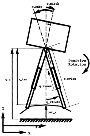
While interactions with the terrain are handled internally, it is nice to see what the robot is doing, and it is necessary to know how far off the ground the robot is. Having access to the terrain variables allows the control system to easily calculate the body height, and it makes it possible to graph the terrain. The following variables are shown in Figures 3-1 and 3-2:
q.z The vertical hip position relative to original ground level. This value is provided by the simulator. However, if more realistic issues such as robustness to sensor noise are important, this data should not be used. Instead the height to the ground should be calculated through a leg which is in contact with it.
termz The height of the terrain above the original ground. This is updated each control cycle to give the height of the terrain directly under the body. No state directly uses this information, but it is useful for displaying the robot's
view of the terrain it walked over.
z_ter The position of the hips relative to the terrain. This is the difference between
q.z and ter z and serves as the robot's measure of body height. A PD controller modifies the desired vertical force on the body to control this height.
3.3
KWALKA
My first approach, referred to as KWALKA, employs revolute hips on the bottom of a block body with prismatic knees. This allowed speedy initial development of a walking algorithm with intent to modify it for uneven ground. Initial work was easier with the prismatic joints for a number of reasons. Problems were more easily diagnosed and offered more intuitive solutions than a system with a revolute joint at each location. The whole structure was easy to directly analyze and tune. The variables measuring joint positions were easily understood, so images of desired behavior were easily quantified and geometric constraints and actuator limits were simple to choose.
Once the high level control had reached stability on level ground, adaptation to uneven ground proved rather trivial. This is perhaps a result of the force-based control when dealing with the ground. Changes required to deal with rough terrain involved checks to guarantee ground clearance on the swing foot, and handle
situ-ations when feet hit the ground unexpectedly. Uphill grades favored shorter stride lengths, while downhill sections were best handled with longer steps. Further work improved the efficiency and reduced peak actuator forces and torques.
The peak actuator output required was of primary concern in developing a real-istic simulation. A robot with an enormous power to weight ratio has little trouble dealing with hills and moving its limbs quickly enough to maintain very high veloc-ities, but real mobile robots have real limits which force the development of more efficient approaches. The key to keeping the simulation realistic was keeping the peak actuator output below the limits on the physical robot. For the hip joints,
this is easily checked. With prismatic knees, however, a constant force limit is not sufficient when trying to emulate a robot with revolute knees. The peak longitu-dinal force a revolute knee can produce is a function of the knee bend. While a peak longitudinal force could be calculated based on imaginary knee bend, the most direct way to emulate the real robot is to reconfigure the simulation.
One may ask why the robot was not built with prismatic knees, if these are sim-pler to conceptualize. Prismatic joints are usually avoided for reasons of complexity and durability of actual implementation. Additional material is required to prevent binding, and the drive system is continually subject to any forces on the leg. Since the power to weight ratio is a primary limitation for mobile robots, designs which require additional material to perform a given task are not preferred. Reliability and mean time between failures is a second issue. Having more parts which are pushed closer to their limits has a detrimental influence on the run time to repair ratio, making a real robot very time consuming to maintain.
3.3.1 KWALKA Variables
The configuration variables of KWALKA are shown in Figure 3-1.
q.pitch Measures the body rotation from vertical, with nose towards the ground
being positive. On a real planar system, this is easily sensed from the planar joint rotation. On a free robot, deviation from vertical would have to be measured with some sort of gyroscope, camera system, or vertical range-finder. Obtaining this data is not trivial, but it is not exceedingly difficult. It is very important information to have.
q.rhip Measures rotation of the hip relative to the body. Rotation under and
towards the rear marks the positive direction. This data is readily available from a potentiometer or shaft encoder on a real system.
q.rknee Measures displacement along the leg axis. Upward motion is positive,
retraction. A variety of linear position sensors could provide this input on a real robot, such as linear pots or magnetic coils,
q.z The distance from the hip to base ground. This is easily obtained on a two dimensional robot, as the vertical motion of the support can be measured; however, one of two different methods would be required on a free robot: Either calculate the ground height through the knee and hip parameters when a foot is on the ground, or add some sort of altimeter/range-finder to monitor the ground height below the body. Precision requirements may force one to use the more complicated method.
q.x The distance from the hip projection on the X axis to the global origin. This
simply keeps track of how far the robot has traveled, but it's derivative is very important for the gait control algorithm. With a boom or treadmill, this is straight forward data to obtain. However, two integrations of inertial data is one of the few ways to measure this in a free robot, and that makes noise a key issue. The algorithm has no need to accurately know the X position, so a real implementation could approximate step lengths if the data were deemed useful. The terrain needs this information, however, and it also allows the
simulator view to track the robot as with walks.
qd.x The velocity along the X direction. This provides input for a first order veloc-ity control in the double support phases. It also is important as a condition to end double support. Once the velocity is sufficient to coast over the lead foot, the trailing leg must enter the swing phase in order to be in place soon enough to prevent a fall.
thetar The angle of the hip relative to vertical. This value increases as the hip swings down and to the rear. It is simply calculated from the global body angle and the angle between the thigh and the body. Position controlling the supporting hip to this value keeps the body near level.
3.4 KWALKB
In order to prove sufficient efficiency, the algorithm was implemented on a second model, known as kwalkb. This model has revolute hips and knees, with the approx-imate geometry, mass properties, and actuator limitations of the physical robot. It required transformations on both sides of the control system to express the actual joint data in terms that the controller understood and to map the controller's com-mands onto the joints. This is a required step for implementation on the actual robot, as well, so it was work necessary at some point. While the controller still operates on a virtual prismatic leg, the actuator limits now correspond directly to those of the actual robot. Now physically achievable performance is easy to verify.
Also, when the controller requests too much torque, motor saturation is now simulated. The maximum torque is provided is fixed, placing a constraint on the maximum virtual leg force which varies with knee bend.
3.4.1
KWALKB Variables
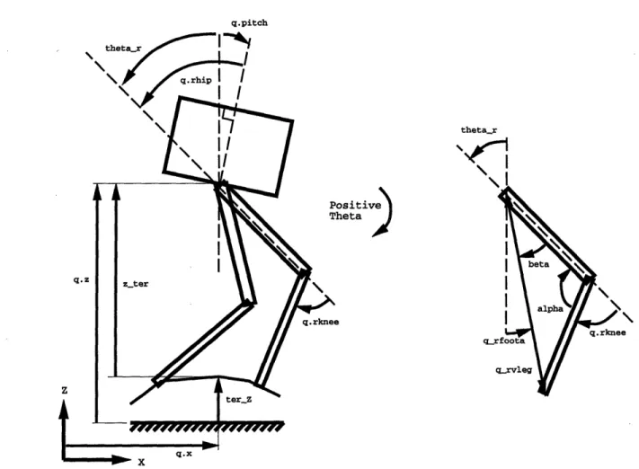
In addition to its configuration variables, KWALKB needs to calculate the data that the virtual leg would provide. All the variables are pictured in Figure 3-2. Only the right side variables are listed, since the same description is true for the left side as well. The physical variables are as follows:
q.pitch Measures body rotation relative to vertical, as on KWALKA.
q.rhip Measures rotation of the hip relative to the body. Rotation under and towards the rear marks the positive direction. This data is readily available from a potentiometer or shaft encoder on a real system.
thetar The angle between the thigh and vertical. This is the same on KWALKA.
q.rknee The outside angle between an extension of the thigh and the shank. This is the angle which fixes the distance between the hip and the foot. As with q.rhip, this is easily measured with a rotary sensor.
q.pitch theta_r
"
A1
sitive leta eFigure 3-2: Configuration and Virtual Variables of KWALKB
q.z Hip height from ground zero. This is the same as for KWALKA.
From these physical values, the controller can compute the data that a prismatic leg would be returning if its end points coincided with those of the real leg. The virtual data is put in the following variables:
qsrfoota The angle a line connecting the hip to the foot makes from the vertical.
From the physical variables, alpha and beta, the upper and obtuse angles in the real leg/virtual leg triangle can be found. These provide an intermediate step to calculate the angle of the virtual leg with respect to vertical using the law of cosines.
qrvleg The distance between the hip and the foot. This is the length of the virtual
leg. Again, the law of cosines can be used to express this length in terms of alpha and the link lengths.
3.5
Servos
In both models, a variety of servos can drive each joint. The default option is a limp servo, which exerts no torque at the joint. The planar joint employs limp servos along the X, Z, and pitch axes. In some states, other robot joint servos are set to be limp to keep foot contacts from generating contending shear forces.
A position control servo uses proportional and derivative gains to control the angle or extension of the joint. This mode is used to put the robot in the initial configuration. Once walking begins, position control is used to move the swing leg and to control the body pitch. The proportional term is closely related to the maximum forces, so the program takes this parameter from the user. In order to achieve the desired damping characteristics, the user specifies a damping ratio, from which a function calculates the required derivative gain.
A third type of servo available is PD position control with a feed forward force or torque term. This mode uses the same gains as the PD mode, but adds the ability
to directly add output torque of force to the PD control. This can shrink the steady state errors when approximate forces can be calculated. The PD control can then correct for errors between the requirements and the estimates, achieving the same total errors with lower PD gains, and therefore, better stability.
A pure feed forward servo is a fourth option. This ignores the position and derivative terms entirely and exerts the commanded force or torque, regardless of where the output is or how it responds.
A final mode is the feed forward servo with damping. The commanded force or torque is applied, but a viscous friction term generates a resistive force proportional to the velocity. This generates a constant velocity servo, which is used to lower the feet to the ground.
Servo outputs are constrained to reasonable limits on KWALKA and to the limits on the actual robot on KWALKB. For KWALKB, this ensures both that controls within the simulator will not exceed the maxima of the real robot and that the simulation's behavior will also predict performance degradation as situational demands exceed the actuators' abilities. Left unchecked, the actuator outputs could be recorded and screened to verify that maxima were not exceeded, but this would not demonstrate what may happen if the real robot is subject to situations which
Chapter 4
The High Level Control
4.1 The Basic Control System
The control system is a finite state machine which cycles through a series of states corresponding to each phase of the walking gait. While entering each state, the joint servos are put into a desired mode. One or more conditions specify when to transition to another state. While these conditions are not met, the joints are controlled as directed by the current state. The controller for both models operates on the distance from the hip to the foot and the angle between vertical and the hip to foot line. This in effect assumes that both models have a revolute hip with a prismatic knee.
For kwalka, this is the arrangement, but for kwalkb, this is a virtual structure. The commands for this virtual leg and the data about it must be transformed to deal with the leg that is actually there. This high level controller computes desired Cartesian forces which are then transformed to desired joint torques or forces. The desired vertical force is computed by a proportional plus derivative controller. It commands a vertical force to maintain the body height at the nominal Z parameter in all states. In single support mode, the only direction of force possible is in the line of the virtual leg. This fixes the ratio of the vertical to horizontal forces, so only one Cartesian force can be controlled in single support mode. By setting the
desired vertical force, body height is controlled, while forward velocity is left to do as it will.
The desired horizontal force is calculated only when both feet are on the ground. A simple proportional velocity controller works to maintain the horizontal velocity at the set-point. The robot's forward velocity slows significantly as it moves over the foot in single support, due to the constant height constraint. Once the body has crossed the foot, it accelerates until the swing leg lands. This controller simply applies a force proportional to the velocity error whenever possible (ie. in double support phases). The maximum horizontal force varies with configuration, so the force is limited at the joint level. When the controller commands too great a hori-zontal force, a net upward force results on one of the feet. The controller assumes that the ground is sticky and can therefore be pulled upon as well as pushed. This behavior is prevented by checking the net force on a supporting foot due to the joints. If this net force ever tries to pull on the ground, the joint commands are
adjusted to maintain a slight downward force on the ground.
4.2
Control Variables
Several variables affect the nature of the walking behavior.
qdd.x Desired X velocity. This parameter is the set point for a proportional velocity controller. The controller uses the difference between this set point and the actual Cartesian velocity to determine the desired horizontal force. In the double support phases of the gait, the weight is distributed between the feet to provide this force while supporting the robot as well.
q_d.z Desired hip height. This input is the set point for a PD controller that calculates a desired Cartesian force to control the robot's height above the ground.
theta-min Minimum forward angle to terminate the swing phase. This parameter specifies how far forward the swing leg must rotate before the swing phase is complete. This corresponds quite closely to stride length.
swinglead The offset used when the swing leg mirrors the support leg. This value is added to the negated support leg angle in order to put the swing leg ahead of being symmetric with the support leg. This allows better velocity control, since the lead leg touches down farther ahead of the body. The widened stride length allows a broader range of horizontal forces to be commanded.
gclearance A vertical offset for the swing leg. The swing foot must clear the last ground contact point by this value before the foot is considered clear to swing.
swinghi A vertical offset that determines the desired swing leg height. The desired value of the swing foot height is set from this offset, which is greater than the g-clearance offset. This puts the leg in motion towards a higher point. The clearance point provides a trigger to begin the swing, in anticipation of where the foot will soon be.
swingh A vertical offset for the swing leg relative to the support leg. On uneven terrain, the swing foot may leave the ground well below the support foot. If the desired position obtained from the swing-hi offset is insufficient to clear the height of the support foot, swing-h is used to find a new desired position for the swing foot.
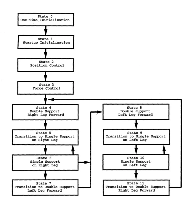
4.3 The States
The finite state machine's states include: initialization, stabilization, and re-peated states for double support, double to single support transition, single sup-port, and single to double support transition. Figure 4-1 summarizes the sequence of states. The repeated states treat the left and right steps separately, so the state
State 0 One-Time Initialization State 1 Startup Initialization State 2 Position Control State 3 Force Control ,i State 5
Transition to Single Support on Right Leg State 6 Single Support on Right Leg
•__••
H-State 9Transition to Single Support on Left Leg
State 10 Single Support
on Left Leg
t
Figure 4-1: The Controller States
State 4 Double Support Right Leg Forward
I
State 8 Double Support Left Leg Forward
State 7
Transition to Double Support Left Leg Forward
State 11
Transition to Double Support Right Leg Forward
I .
- I .
completely summarizes the phase and lead leg in the gait. This proved to be more straight forward, although somewhat repetitive.
4.3.1
Before Checking the State
There are a few calculations which are the same for all states. Rather than repeat these inside each state, they appear in adapt-control, which is called at the beginning of the control loop, before the state is determined. Two of these items use the rough terrain function to interpolate the current terrain height under the body, and update both the altitude of the terrain and the body height relative to it. Although the terrain altitude is not used in the control, it is useful to be able to graph the robot's perception of the ground height over time. I also used the difference between the ground height and the robot height from ground zero to fill the relative body height field. This information can also be calculated from the joint positions, as long as the feet are on the ground. I chose the absolute height differences because it simplified the expressions. This absolute measure of body height would be difficult to implement without very precise altimeters, it serves the same purpose as the more direct method of calculating the height from joint angles. If the robot model introduces noise in sensors and actuators, the joint angle calculation must be used to be consistent with the model.
The adapt-control function also computes other information, useful to the con-troller and to the observer. The angle and distance of each foot relative to the body is updated here, as well as an estimate of the terrain slope and the coefficient of friction each foot is experiencing against the ground. While some of this information
is not directly involved with the control, it is useful to have available when assessing how realistic the simulation was.
4.3.2 Initialization and Oscillations
States zero through three perform a series of set up and waiting functions which put the robot at rest before the walking algorithm begins. State zero performs all the one-time initializations, setting constants from the header file parameters and setting up the initial state. Setting globals to the #defined values seems redundant, but this allows initial values to be kept in the header file, away from the tangle of controller code. Making them globals allows them to be viewed and changed at any time in the simulation. This is an advantage when searching for correct parameter values to tune the behavior.
State one performs the detailed initialization and goes on to state two, which updates the knee commands to follow any user changes in the desired z height. After a brief delay, all joints are switched into force control mode, and the knee position gains are reduced, since position control is only used to move the knees when they are in the air from this point forward. The damping required to roughly achieve the desired damping ratio at each joint is calculated for the new gains. Finally, the desired Cartesian forces are calculated and then transformed into joint forces. This state waits for a moment so that any oscillations in the force control can settle out. Then walking can begin.
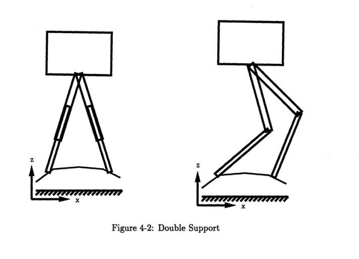
4.3.3
State 4: Double Support, Right Leg Forward
In the double support phase, Cartesian forces in X and Z are commanded. The lead leg's hip is position controlled to stabilize body pitch, but only while the lead foot is in contact with the ground. This check prevents hip torque from slamming the foot down if it bounces. The body tends to pitch forward in the single support phase as the swing leg is servo-ed forward. Thus, using the lead leg to correct this increases the downward pressure on the lead foot, while the trailing foot would lose contact pressure if that leg were trying to correct the positive pitch error. Therefore, the trailing leg's hip remains limp to keep the trailing foot on the ground while
Figure 4-2: Double Support
preventing internal forces from horizontally loading the feet.
Both knees operate in feed forward mode throughout the double support phase. Having set the hip torques as above allows feed forward forces or torques for the knees to be calculated from the Cartesian force equations, completing the transformation from desired Cartesian forces on the body to joint commands.
The trailing leg is vital to contribute horizontal velocity during the double sup-port phase. Once sufficient velocity exists to coast over the supsup-port leg with a specified minimum velocity, the trailing leg can be lifted. This condition is devel-oped by integrating the horizontal force acting if the lead leg were to support the weight of the robot and rotate from its current position to vertical. This is the energy that will be subtracted from the current kinetic energy. Since the vertical height is held constant, the kinetic energy at vertical will be the current kinetic minus the work done by the lead leg.
immediately. Once this final velocity clears the minimum velocity parameter, the trailing leg should enter the swing phase so that it can be in position to begin the next double support phase before excessive velocity develops from having the single support leg behind the body. This calculation does not factor in the deceleration from driving the swing leg forward, so the actual minimum velocity dips below the minimum velocity parameter. It is a sufficiently small error, however, that the
minimum parameter can be adjusted slightly higher to compensate.
Time spent in the double support phase can both accelerate or decelerate the body to bring it back to the desired velocity, depending upon which leg contributes more vertical force. As this happens, the minimum velocity condition becomes less demanding because the lead leg continues to rotate towards vertical. Eventually the minimum velocity condition should be satisfied, and control will switch to state 5. As a precaution, state five will take over if the support leg crosses vertical even if the condition is not satisfied. This case is only useful for real time control. It is likely to help the robot regain a stable gait if it has momentarily exceeded the algorithm's maximum velocity. It is quicker to skip to the next state after a direct comparison than to evaluate the minimum velocity expression first.
4.3.4 State 5: Double to Right Support Transition
The principle role of the double to single support transition is to lift the trailing leg off the ground so that it may enter the swing phase and servo forward to prepare for the next double support phase. The lead leg acts as if single support has begun. The horizontal force is ignored in order to maintain the proper vertical force. The body pitch is controlled by servoing the lead leg's hip, as in double support.
The trailing leg is servo-ed to raise the foot to a required ground clearance so that it will not hit the ground in the swing phase. With the prismatic knees, only the knee is position controlled to lift the foot and the hip is left limp. The revolute knee version uses action from both the hip and the knee to lift the foot off the ground along the angle of the virtual leg.
z
Figure 4-3: Transition to Single Support
The single support state is entered when the rear foot has been lifted higher than the larger of the lead foot height or the minimum ground clearance and the rear foot switch shows no ground contact.
4.3.5
State 6: Single Support on Right Leg
The single support phase simply rides out the transition of lead legs. The support leg's knee is force controlled to maintain body height, while the hip is position controlled to keep the body level. The swing leg is position controlled at both joints to keep the foot above the last ground contact or above the supporting foot by the ground clearance factor. The swing leg also positions the foot to mirror the angle to the support foot, plus a lead factor. This smoothes the transition from trailing leg to lead leg.
Once the swing leg reaches a minimum forward angle, the swing phase is com-plete, and the transition to double support happens in state 7. If the swing foot hits
--z
Figure 4-4: Single Support
the ground early, one of two actions is taken. If the swing leg is ahead of the support leg, this simply means that the transition to double support has already occured. The transition state is skipped, and the next double support phase is begun in state 8.
If the swing foot hits the ground while it is behind the support leg, a little stumble is executedj by jumping back to state 4. A severe toe-stub can remove sufficient energy to make it impossible to maintain vertical height and rotate over the support foot. By returning to the double support phase, the controller can try ensure there is sufficient energy to coast across the support leg. If the foot hits too far forward of the body, the is no chance to inject additional energy. A backwards fall is then unavoidable without quickly repositioning the feet.
z
-z
z
X X
Figure 4-5: Transition to Double Support
4.3.6 State 7: Right to Double Support Transition
This state is responsible for putting the swing leg back on the ground. This issue is somewhat complicated because the ground elevation beneath the lead foot is not known. To surmount this lacking information, a constant rate of descent is used to lower the foot until it hits the ground. The rate is chosen to be as quick as possible without excessive bouncing, and is set by the combination of a feed forward force and a damping constant. Once the foot registers ground contact, the next double support phase begins.
4.3.7
State 8: Double Support, Left Leg Forward
This state repeats the calculations of state 4, but with the left and right roles ex-changed. The left hip now controls the body angle while the right hip remains limp. More speed is provided by biasing the weight to the right foot, while deceleration is
caused by biasing to the left foot. The energy calculation triggers the transition to
state 9.
4.3.8 State 9: Double to Left Support Transition
While the right hip remains limp, the right foot is lifted from the ground. Once it sufficiently clears the ground or the left foot, single support on the left leg is controlled in state 10.
4.3.9 State 10: Single Support on Left Leg
Single support is executed on the left leg, simply mirroring the conditions and controls from the right leg support. The state can switch to 11 if the swing leg reaches the minimum swing angle, to 4 if the foot hits the ground in front of the support foot, or to 8 if it hits behind.
4.3.10 State 11: Left to Double Support Transition
As before with the right to double support transition, the swing foot is lowered to the ground, and double support in state 4 begins once contact is made.
Chapter 5
Results and Observations
The final performance of both models was quite surprising. Once the algorithms performed on smooth, flat terrain, bumps and significant hills required little more than tuning some parameters. A few new state transition conditions were added to remedy failings which were due to improper state assignment. These new conditions included issues like choosing which state to enter after single support if the swing foot hits the ground before reaching its goal angle. A few bugs in condition calculations even crept out towards the end when an improper variable was used in place of one that measured a similar, but different, value.
For this discussion I will divide the terrain into three main types: terrain with no net slope, terrain with a net up component, and terrain with a net down component. Each type can be smooth or rough to varying degrees. Data is shown from smooth, rough, and very rough versions of level terrain and smooth slopes. The up and down slopes represent the maximum steepness for which I could tune the individual models.
In general, the desired X velocity is kept low on all terrains. This always keeps the maximum forces lower, and it also keeps descents under better control. The double support phase attempts to prevent the velocity from ever falling below the minimum specified, but its prediction of the velocity after lifting the rear leg is based only on the robot's mass and the action of the support leg. There is a rather
significant reaction to the swing leg motion which makes the actual velocity in the swing phase drop lower than anticipated. The .3 m/s minimum I used in all cases proved adequate to prevent a backwards fall, but it was more like specifying the average velocity than the minimum.
5.1 Level Terrain
On level terrain, step length can be kept at a moderate size and the ground clearance variables are kept small. Short steps make for the most efficient motion, since the support leg must do little more than maintain its length, but the robot must then cope with more interactions with the uncertain terrain. If the step is too short, the robot can easily be upset by a drop in terrain, since that results in additional forward velocity that must be controlled by biasing weight to the lead leg in double support. If the lead leg is not sufficiently far ahead, the velocity cannot be reduced to the desired level. After a few steps this velocity can build out of control until the swing leg can no longer reach a position in front of the robot before it hits the ground.
If the lead leg swings too far forward, a down hill slope causes a fall. The leg cannot reach the ground after the swing phase, and the robot has to leave the leg extended and wait to fall onto it. This is usually catastrophic.
Keeping the swing leg close to the ground helps smooth out the transitions into and out of double support. This reduces the delay between the decision to pick up or put down a foot and the completion of the action. The conditions for lifting or putting down a foot neglect the transit time. At significant swing heights, this can become a significant factor in the ability to control the velocity.
An additional set of factors with great significance for the stability of the gait is the swinglead and theta-min combination. If the swing lead is too large, the steps become very long. To accommodate long steps requires additional power or significant body bounce. When the lead is too small, the swing leg gets behind,
and the velocity goes out of control. Thetanin couples with swinglead to find a balance between the control of the velocity and the efficiency. While no direct efficiency is calculated, the maximum torques and forces available from the joints prevent grossly inefficient gaits from being stable for long.
5.1.1
Smooth Surface Performance
Performance on smooth terrain was very good, but it did seem to suffer from the precautions present for handling rough terrain. Figure 5-1 presents the data sum-marizing the behavior of KWALKA on smooth, level terrain. The body exhibits small oscillations just above the set point. These are due to the simple PD height controller. It reacts to deviations caused from imperfect knee forces and commands more or less total vertical force to correct for deviations from the set-point.
The positive steady state error is due to an over estimate in the approximation used in calculating the force due to gravity. The thigh masses are being supported by the knee joints, but usually at an angle off vertical. Therefore, the linear joint structure is bearing some of the load, and the knees would not have to bear the entire weight. The calculations treat the force due to gravity as a constant and set the knee forces to counter it at all times.
The horizontal velocity exhibits oscillatory behavior for an unavoidable reason. The system is under actuated in single support. The vertical position control is given pressidence over the horizontal velocity, so each swing phase was expected to cause the velocity to fall and rise again. With no terrain disturbances and the small step length this run used, the double support states do not last long enough for the robot to achieve the desired horizontal velocity. Then, the velocity dips below the set minimum value because of the neglected swing leg interaction. This actual lower bound is a function of the swing leg mass properties and the forces applied to it. Since this is a constant offset, the minimum velocity set-point must be high enough to accommodate this loss.
0.5 1 1.5 2 Distance in Meters 2 4 6 0 2 4 6 V. a 0 2 4 0 2 4 Time in Seconds 0a) 0 LL 0 a Ye 0 2 4 20 T5 10 < 0 -o -20 6 1 Cl) 0. :3 >0 O. , 2 f 6 6 0 2 4
I
: :
!
t[
i:
i' ' I i 1 i i i1
,,b P. I, ;'· i % G " f % s* · ·-- -· .. ,· ,· 5 r ·d h· r.' r\ :I r·· r.· ) U-0 2 4 Time in Seconds 6Figure 5-1: KWALKA on smooth, level ground. All units in MKS, with angles in degrees. Dotted traces indicate the left side for leg data graphs.
0.4 x 'a N 'U, n 00.6 -o 0.4C (U N 0.2 ~.1 (D 1 V 0 a 0.55 N 0 0. 2 A 0 2 10 (U
05
C co Q. -Y? 4 4 1 -1 6 6 .. .... ' · · . · a) 0 I -.: 0 2 U.00 0.6 0) > 0.55 0.5 VVV\V\FWW\V\F\F~V 0 U. 0 LL C O(Uo
....ffifimm
· Jr i4lt.A:·A64MWM1.1 ·IU. N I I U.A) - -- - - - -·V
,, · · · U% I a* s " ' · n· rr · · II.- la ·. II · · ·· Ir · iEach drop of the state from 11 to 4 represents two steps. In this trial, the double support periods account for nearly half of the cycle time. Over half of the remaining time is spent in the single support phases. The short stride length and low ground clearances used here make the transitions between support modes very short.
In order to obtain sufficient joint velocities, the joint damping had to be kept quite low. This results in pitch oscillations in response to the swing leg movements, which remain bounded between plus and minus 3 degrees.
The hip torques remain between the bounds, except for a single spike at the onset of a right foot swing phase. The hip torques are limited by clipping desired position commanded to keep the hip response within the torque limits. This does not account for the derivative term in the controller, which provide an opportunity for the hip torque to momentarily exceed the defined maximum limit. Adding the
derivative term should keep the limits more strictly enforced. Since the knee forces are directly commanded, they are kept strictly within the defined limits. The forces are quite biased in the downward direction, which may make designs which take advantage of this more efficient. A symmetric drive costs additional weight for force potential in directions that are not used.
The parameters tracking the virtual leg-in this case, the actual leg-are also shown. The small deviations in leg length and small motions of the feet summarize this gait's small power expense.
The Cartesian forces act as expected. The vertical force hovers about the weight of the robot. Small deviations in vertical height require only minor adjustments in this direction. The horizontal forces peak at the onset of each double support state. This indicates that significant velocity is being lost in the swing phase each time. The magnitude decreases to a steady state level after the first few steps. A larger gain on the velocity controller could reduce the steady state error, but the
step length is a primary limitation on the settling time.
The final plot displays the effective coefficients of friction for the left and right feet. It goes to zero when the foot is off the ground. This is monitored by the
foot switch variable for each foot. The forces seem to dissipate out of proportion, however, and a delay in registering foot separation from the ground causes spikes each time a foot is lifted. Without the spikes, this gait requires a friction coefficient of at least .2.
The results for KWALKB on smooth, level ground are shown in Figure 5-2. Better control of the swing leg angle gave this run a longer stride length. This improved the horizontal velocity control but degraded the vertical stabilization. The velocity control was nearly perfect, with the range only slightly exceeding the desired max and min settings. This is likely due to the slightly lower body height than desired. The anticipated loss of energy is not as great as actual, so the disparity between the actual minimum and the desired minimum goes away.
The torque limits on the knees cause a more stringent limitation on the maximum virtual leg force that becomes worse with knee flexion: The more the knee bends, the less force the virtual leg can produce. The stride length limits the body height set point, since the feet must reach the ground at the limits of the step. This forces the knees to operate at a large enough flexion to make the virtual leg much weaker than on the prismatic model.
The Cartesian forces also show greater variation due to the wider stance. While the vertical force changes significantly, the desired horizontal force eventually shows only small spikes to restore energy lost in the step. While the desired horizontal forces are smaller, the applied forces are larger because of the wider stance. This drives the required coefficient of friction up to at least .4 at the start.
5.1.2 Rough, Level Terrain
The next set of tests were run on a randomly generated terrain spanning a list of points 0, 1, 2, 3, and 4 cm high. This required additional swing heights and swing leads to prevent tripping or stubbing the feet on the bumps.
KWALKA showed significantly larger altitude variations on this terrain. The terrain changed faster than the altitude controller could respond since each step put
0 0.5 1 1. Distance in Meters V.0. 0 0 2 2 4 4 5 2 0.4 x 'a 0.2 0 10 5 0 CL 6 6 0 2 4 ( 0 0e 0 a) 2 4 0 2 4 6 6 20 *- 10
0
,o -10 -20 2 4 2 4 6 Time in Seconds 1 ci, >00.5 2O~ n Ci...h
M z A' A.
A . . J A 2 4 Time in Seconds J,.,,, I A AkJ J \ 6Figure 5-2: KWALKB performance on smooth, level ground. All units in MKS, with angles in degrees. Dotted traces indicate the left side for leg data graphs.
N ', 0 , 0.6 0 rr -a 0.4 N102 0 A V.U A}0.55 N I.
J
_V
f___vvv\___
v
10 0 0 --10 (0) 0 .. I >1 0.6 0.55 0.5 V..tij 0 2 4 . , .. 0 8 100 ( o LO C _ 0 o -1000 0 6 . : I . : . - : - - . : '. . 'I : : ., :·· - - - -F"I\ · . `'"'"" LiY-L.- ·· ... .. . .... ....A.., I nA 11M I m I . AjI _ .,B vV 0.1 - AP " ' 6 O I ) · · A- ';'the foot at an unpredictable new height. The longer stride length kept the velocity under control, despite the sudden drops encountered in the terrain. The velocity regularly dips lower than it did on smooth terrain, but each double support phase manages to restore it to the set-point.
Double support takes up a longer segment of the stride cycle because the lead foot lands farther ahead. The pitch oscillations oscillate with the same magnitude, but are now biased slightly negative. Hip and knee torques are more widely varied than they were on smooth ground, but the average magnitudes only increase slightly. What changes significantly is the range of leg lengths. This is due in part to the longer stride length. The uneven ground causes additional modulation, making for marked increases in the motion of the legs. This test demanded much greater energy output from the robot.
Other new features this behavior exhibits are the zeroing of the desired horizontal force and the oscillation evident as the legs swing forward to -10 degrees. The longer strides cause both of these features to appear. The required friction has grown from the smooth ground case as well. There are fewer extraneous spikes, but the valid sections are higher.
Figure 5-4 shows the results of sending KWALKB across the rough terrain. Comparison with the smooth terrain test shows an increase in altitude variation, although it is always below the set-point. The gait cycles become less regular, and some of the double support phases lengthen considerably. The velocity remains very well controlled, with a slight variation beyond the bounds after a significant bump. Hip torques actually drop, and knee torques remain about the same. The last step with the right foot lands hard, as can be seen from the larger knee torque commanded at that point.
The range of virtual leg lengths and angles expands dramatically. This is mostly due to the lead leg taking a long time to come down when stepping into a depression, because the foot continues to move forward as it descends. The friction demands increase rather dramatically as well.
N Vt 0 .a 0.60 n: · ' 0.4 CU N 0.2 1 0) 0 0.5 1 1.5 Distance in Meters 0 2 4 x 'O 0.4 0.2 0 0 2 4 E 10 o 5 C _ 0 a. 6 0 a) 10 (D 2 0t U-0 2 4 6 2 4 6 0 2 4 6 2 4 ( 2 4 Time in Seconds 6 ' 10 C< 0 0 t -10 -20 1 ! 0.5 0 0 2 4 E
iM
Time in Seconds 6 0Figure 5-3: KWALKA performance on rough, level ground. All units in MKS, with angles in degrees. Dotted traces indicate the left side for leg data graphs.
1 '~ 0.55 N 0. a0 > 0.55 0" 0.6 0.5 20 0 0.45 a, 100 -100 0 C lo 0 r ~ r~~~~~~~~~~~~ I -~_ - _ ;r _ I . , .~ ~ ~ ~ ~. ~ . F * _ I %~~~~~~~~~~~~~~~~~ . .·· ...... ·.. ·.... '· · ' · · ·-"··' · ··._·:····1.-···. '· ·' - '· '' A. , _ , ._ . .~-, , _ ._ . w _ I ·.... ,...
.:... ..
c a\ 1 2 6 0.6 r rr PA U.0: 6 I 6 2 4 .... " ' ' ' ' '''" .. ·· rl ·. . .I · .· · ul I ·· · · v · r .·. - vr r · · vl · r · ·.1 1.5 2 Distance in Meters 4 4 4 x -o V 0 2 4 1 0 C.
0
6 0 20 0 2 o 0 C -10 -20 6 6 0 0 2 4 2 4 2 4 2 4 Time in Seconds c) co 2 :3 :E 6 1 0.5 0 0 2 4 Time in SecondsFigure 5-4: KWALKB performance on rough, level ground. All units in MKS, with angles in degrees. Dotted traces indicate the left side for leg data graphs.
N u. . 0.6 -O.4co0.4 N1 0.2 1-1 (D V 0 0.5 0.t N0.55 0 0 0 0.
I
10 0 -10 I 0 2 2 2 6 6 6 6 0.65 0.6 0) - 0.55 0.5 nfl A 0 100 ,o " 0 Co -100 C) 0 6 hi · · " '' ' · '· '· '" ·- · · · '' :. ·'· " '' ·. ... '· .· · · r · . . ~~~~~~ .~~~~~~~~ -I·.
·
~
'-.W.
A... I.-N -~~~~~·
o .. ... I I... · n A .v I n L IComparison of the two models on the rough terrain shows considerably less ve-locity and pitch deviation in KWALKB. The hip torques are lower, and the height varies by about the same amplitude. The revolute knee model shows greater varia-tion of leg length and angle, however. This can cost addivaria-tional energy. The efficiency comparison is somewhat clouded by the greater hip torque in the prismatic model, though. KWALKB's steps are longer and the average desired horizontal force is much lower. It does demand greater friction, however.
The next piece of terrain doubled all the heights of the rough terrain to produce very rough terrain. The grid points defining the terrain are 0, 2, 4, and 8 cm above the floor. KWALKA shows similar changes to those between the smooth and rough tests. The only notable increase is on body height control. The friction requirements grow noticeably as well. The commanded knee forces are slightly larger, and the virtual leg lengths and angles also increase by a small percentage. Figure 5-5 shows summarizes the results.
KWALKB shows a much more dramatic difference between its rough and very rough terrain performances. The vertical position error is much greater on the very rough terrain, and the knee torque increases enough to saturate on the last right foot step. The added vertical deviation aggravates the leverage disadvantage the knees experience. The velocity swings up by more than 40 percent stepping off a bump at the end.
Compared to the performance of KWALKA, the minimum velocity is better regulated, but the maximum velocity is less controlled. The vertical deviations are greater and still centered below the set-point. Hip torques are still significantly smaller, but virtual leg motion is considerably larger. More friction is required.