Asset liability management throughout macroeconomic cycle in financial institutions

Asset Liability Management throughout Macroeconomic Cycle in

Financial Institutions

By

Jingsi Yan

B.E. Computer Science & Engineering P.E.S. Institute of Technology, 2002

SUBMITTED TO THE MIT SLOAN SCHOOL OF MANAGEMENT IN PARTIAL FULFILLMENT OF THE REQUIREMENTS FOR THE DEGREE OF

ARCHNES

AT THE

MASSACHUSETTS INSTITUTE OF TECHNOLOGY JUNE 2013

02013 Jingsi Yan. All rights reserved.

The author hereby grants to MIT permission to reproduce and to distribute publicly paper and electronic copies of this thesis document in whole or in part

in any medium now known or hereafter created.

MASSACHUSETTS INSTiiTE oF TECHNOLOG0Y M

k-MAY 3 o 2

BRA R IF S

MIT Sloan School of Management May 10, 2013

Certified by:

Xavier Giroud Ford International Career Development Professor of Finance Thesis Supervisor

Accepted by:

Michael A. Cusumano SMR Distinguished Professor of Management Program Director, M.S. in Management Studies Program MIT Sloan School of Management

Asset Liability Management throughout Macroeconomic Cycle in

Financial Institutions

By Jingsi Yan

Submitted to MIT Sloan School of Management on May 10, 2013 in Partial Fulfillment of the

requirements for the Degree of Master of Business Administration.

ABSTRACT

In this thesis, we are going to study asset liability management throughout the macroeconomic cycle in financial institutions. There are two important problems in financial institutions. The first is that asset and liability management has significant effects on the financial institution's value. The second is that in different stages of the macroeconomic cycle, the effect of asset and liability management approaches is not same. Therefore, the purpose of the thesis is to study how asset liability management causes economic consequences for financial institutions and in what capacity. In this thesis, based on the analysis of asset liability management and the economic cycle, we establish a dynamic system to simulate how a financial institution makes decision throughout economic cycles. In order to simulate the system, we established a model to reflect how the economic cycle affects the financial institution's value by using the economic

relationship and we built up the decision making progress. Then we simulate the system through Matlab. From the simulation results, we can observe the changes of system in the given time horizon.

Thesis Supervisor: Xavier Giroud

ACKNOWLEGEMENT

I would like to express my deepest appreciation to my thesis advisor, Professor Xavier Giroud

from MIT Sloan School of Management, for his guidance. His patience encouraged me to explore more on this work. His quick response inspired me to improve my efficiency. His research attitude conveyed a spirit of positive energy from academia.

I would like to thank Chanh

Q

China Life colleagues, for their insightful comments and suggestions on formulating my thesis topic.

A special thank you to my husband Zhenwu Shi, who has continuously helped me improve my

capability of critical thinking. Many many thanks to my parents, grandparents and brother, who have always stood by me.

Table of Contents

. Asset Liability M anagem ent Introduction ... I 1.1 A LM -an innate issue in financial industry ... I

1.1. I Profit generation in financial institutions... 3

1.1.2 Risks in financial institutions... 4

1.1.3 Mismatch between asset and liability arrising from the profit model of financial institutions...5

1.2 A sset liability m anagem ent (ALM ) developm ent... 6

1.2.1 Role of A LM in m anagem ent of financial institutions ... 6

1.2.2 A typical ALM system in practice ... 7

1.2.3 Developm ent of A LM theory...8

2. Econom ic Cycle Introduction ... 10

2.1 The pain of the recent financial crisis ... 10

2.1. 1 The disaster in recent worldw ide crises ... 11

2.1.2 The asset liability m anagem ent of financial crisis in 2008 ... 12

2.2 The econom ic cycle ... 14

2.2.1 The history crises ... 14

2.2.2 A LM at different stages in the econom ic cycle ... 15

2.2.3 The econom ic cycle research ... 18

2.3 Fisher's opinion on the econom ic cycle... 19

3. A LM M odel throughout the Econom ic Cycle ... 21

3.1 G eneral A LM Decision Progress ... 21

3.1.1 A LM decision point ... 21

3.1.2 Decision of funding...22

3.1.3 Decision of asset allocation... 23

3.1.4 Decision of liability cost ... 24

3.2 Characteristics of A LM m odel...24

3.2.1 A LM m odel key factors ... 24

3.2.2 Econom ic environm ent key factors... 25

3.2.3 Em ploying A LM decision in the econom ic cycle... 26

3.3 A LM Econom ic Cycle M odel... 27

3.3.1 The planning horizon of ALM ... 27

3.3.3 The decision process... 30

3.4 Simulation... 33

3.4.1 Flow chart of A L M m odel ... 33

3.4.2 Scenario G eneration ... 34

3.4 .3 Sim ulation R esult... 36

3.5 C onclusion ... 37

Appendix... 38

1. Asset Liability Management Introduction

In this part, we describe how a financial institution generates profit and what kinds of risks it faces in its business. Then we point out that the profit generation method of financial institutions is the reason for the mismatch between asset and liability. After that we come to conclusion that asset liability management is an innate issue in financial institutions and ALM plays an important role in financial institutions' daily operation. Finally, we summarize asset liability management theories and introduce a typical asset liability management system.

1.1 ALM -an innate issue in financial industry

The financial system has a significant impact on the economy in the contemporary world. The financial system was created to efficiently transfer money between

investors and borrowers. As a result, high leverage ratios and a large amount of liabilities on balance sheets is the most prominent characteristic of financial institutions, such as banks, insurance companies and pension funds. Such kinds of characteristics determine that their balance sheet management should be different from industrial enterprises in terms of the different risks implied in the balance sheets (Danielsson, J. et al. 2011).

In the majority of non-financial industrial corporations, the core operation of an enterprise is to manage the assets to generate sustainable profits in order to maximize

benefits to shareholders. The liability side is used as a tool to reach certain optimal

leverage ratios. In corporate finance, given a net present value (NPV) project,

management will make financial decisions on the financing structure to determine the

relative mix of equity and debt on the liability side (Danielsson, J. et al. 2011). Based

on the situation above, asset liability management in non-financial industrial

corporations can be considered as a decision-making process that goes to the core

operation of an enterprise, in order to support the main source of its revenue, but not

its key profit-making business.

In financial institutions, the role of asset liability management is different from its

supporting role in non-financial institutions that we discussed above. It becomes the

main source of a financial institution's revenue. Financial institutions pay much

attention to the liability side and asset liability management because financial

institutions generate profit from simultaneously managing both assets and liabilities.

Asset liability management will be directly determined in a project but not an

alternative financing choice once a project has been decided to be undertaken. That is,

asset liability management is a core operational process in order for a financial

Figure 1. Typical Balance Sheet for Non-financial Enterprises

Manage physical asset to

generate proft _{> :- the physical asset operation}Manage Libility to match up

Figure 2. Typical Balance Sheet for Financial Institutions

Manage both asset and liability to generate profit

Financial Asset

Liability

Equity

<--Higher leverage ratio

1.1.1 Profit generation in financial institutions

Typical financial institutions generate profit from the difference between the interest

earned by assets and the interest paid to debtors. The spread between return of the

assets and the cost of the liability determines the profit margin for a financial

institution. For a bank, its profits come from the difference between how much it

earns from the deposit through investing its assets or lending loans and how much it

pays to the savers. For an insurer or a pension fund, profit comes from the difference

between how much they earn from managing the assets and how much they pay to the

Liability Physical

Asset

this amount should be recorded in the current liability and future sequent liability.

The insurer will earn the difference between yields of this amount and the implied

interest of that policy during whole period while this liability exists in its balance

sheet.

1.1.2

Risks in financial institutions

Financial institutions face various types of risks in the business world. The main

risks facing financial institutions include market risk, credit risk, liquidity risk,

operation risk and business risk (Zenios, S. A., & Ziemba, W. T. 2006).

Among these risks, liquidity risk is the most vital factor which directly leads a

company to bankruptcy. Liquidity risk is defined as the situation faced by a company

when it cannot raise cash to maintain its normal operations or when it lacks money to

execute a transaction under previously signed contracts. The liquidity risk comes

from the mismatch between the cash-on-hand and the redemption of potential liability,

which is determined by improper asset liability arrangement.

Market risk means that the return of prices of assets and liabilities change from time

to time due to market fluctuations. When the market fluctuates, the changed value of

the asset price or the return cannot be the same as the changed value of the liability

price or return. So the market risk brings a mismatch between assets and liabilities.

Credit risk is used to described the non-payment or potential non-payment of an obligor (counterparty, issuer or borrower) when their ability to make future payments is downgraded or questioned. When the credit default happens, the gap between assets and liabilities will suddenly appear, as the expected future cash flow from the credit products held by the financial institution will be reduced.

Operational risk is the loss resulting from people, systems and processes such as fraud or law suits. The loss from operational risk also will damage the balance sheet and also result in a mismatch as the loss negatively impacts the value of the asset and decreases future cash flow.

Business risk is the uncertainty of the margin or danger of loss in terms of the firm's business. Such kinds of business uncertainty will bring volatility to the asset liability situation and amplify the mismatch.

Based on the above analysis, some risks cause the mismatch, and the mismatch also reinforces these risks and amplifies the negative impact of these risks. To avoid such

mismatches, for several years, financial institutions have used asset liability

management to reach "risk neutral", which means the risk implied on the asset side is equal to the risk implied on the liability side.

1.1.3 Mismatch between asset and liability arising from the profit model of financial

Financial institutions' business is to provide services for packaging and selling risks

to the clients (Zenios, S. A., & Ziemba, W. T. 2006). When a financial institution

sells its products, it collects funds today and enters into a contract which commits

itself to providing future cash flow to its clients. On the balance sheet of a financial

institution, the asset side reflects current funding from financial products and the

liability side reflects future risks to pay the cash flow. The current return from the

asset side is used to pay the liability interest in the past and will be reserved to pay the

liability interest in the future. When the current interest rate changes, the difference

between the risks implied to assets and liabilities will expand. So the mismatch

between assets and liabilities is an innate problem for financial institutions.

1.2 Asset liability management (ALM) development

1.2.1 Role of ALM in management of financial institutions

Asset liability management is the management approach of managing risks from

mismatches between the assets and liabilities of enterprises. The goal of traditional

asset liability management is to align the risks from both sides to reach risk neutral.

Asset liability management focuses on both sides of the balance sheet. Different risks

should be assigned to both sides. On the asset side, asset liability management

focuses on market risk, credit risk and liquidity risk. On the liability side, it focuses

on volatilities of margins and liability costs (Zenios, S. A., & Ziemba, W. T. 2006).

The unique characteristic of financial institutions' balance sheets as described above requires financial institutions to place more focus on ALM. ALM becomes the most fundamental element of the management of financial institutions' daily operations.

1.2.2 A typical ALM system in practice

A simplified asset liability management system is constructed by data storage

analysis tools and reporting facilities, described by the Figure 3 (Zenios, S. A., & Ziemba, W. T. 2006).This framework of an asset liability management system can simulate the performance in order to align assets and liabilities.

Figure 3. Comprehensive Framework of ALM

Data Obligation details Market situation Asset details

Analysis Tools

Risk Measurement Risk Management

Revaluation Hedging

VAR analysis Optimization

Scenario analysis

Reports Financial Statements VAR

The necessary data should be input to compose an economic environment with the

contractual obligations, market information and the business situation. The data is

then used to perform risk measurement and risk management through analysis tools.

Then the results of the analysis form the reports of economic value and risk neutralize

(Zenios, S. A., & Ziemba, W. T. 2006). This ALM framework can provide a view of

the future balance sheet of a financial institution and offer the evidence of their

financial decisions.

1.2.3 Development of ALM theory

The history of asset liability management can be dated back to the 1950s when

Markowitz contributed asset allocation theory. Since.then, a huge amount of research

has been done to develop asset liability management theory. There are typically four

kinds of models classified by time period and uncertainty: single period static model,

single period stochastic model, multi period static model and multi period stochastic

models (Zenios, S. A., & Ziemba, W. T. 2006).

Single period static model: a static model does not count the effects of the random

variable. The return of the asset and liability is static. A typical single period static

model will assume a term structure of asset and liability both of whose durations are

matched. When the assets and liabilities are changed, the term structure will change

by the same amount with the same direction, and such kind of movements happen

independently.

Single period stochastic model: a stochastic model allows the input of a certain distribution of assets and liabilities at different market situations. A stochastic model can explain the correlation between the movements of assets and liabilities. A typical single period stochastic model can construct a portfolio that will have a certain distribution of gap between asset and liability returns in different scenarios under market scenarios. These scenarios will incorporate the correlations of different economic factors which affect asset and liability returns in the time horizon.

Multiperiod static model: a multi period model counts the portfolio rebalancing at certain time horizons. However, the portfolio in a multiperiod static model is rebalanced in the static point, which is not realistic.

Multiperiod stochastic models: a multiperiod stochastic model considers both asset and liability returns movements under certain distribution dynamically throughout the whole time horizon. It provides a framework to simulate the realistic asset liability management problem through realistic simulation to help the financial institution define a strategy resolve the problem (Zenios, S. A., & Ziemba, W. T. 2006).

2. Economic Cycle Introduction

In this part, we start with the pain of the financial crisis to illustrate the failure of normal ALM in extreme circumstances. Then we discuss the different characteristics of stage economic cycles and how these affect ALM. After that, we summarize related economic cycle research. Last, we introduce Fisher's explanation about the economic cycle, which is used to construct the model later.

2.1 The pain of the recent financial crisis

Crisis is an extreme situation of the economic cycle. The financial crisis is the most common manifestation in the crisis stage of the economic cycle. When the crisis happens, all the assets, especially the financial assets, lose a large part of their value. There are a number of different types of financial crisis. One is the bank crisis when banks run out of liquidity or are trapped in related difficulties. Another is the

speculative bubbles and crashes when the stock market or real estate market collapses. Currency crisis is another type, when the currency devaluates suddenly.

The 2008 financial crisis reminded us how fragile the economy is. The economy always experiences cyclic periods of good and bad times. However, the economic cycle is not a regular fluctuation. Two cycles are never similarly repeated

recession, recovery and boom from the trough to the peak. Crisis is the extreme stage that drags the peak down to the trough quickly in the economic cycle.

2.1.1 The disaster in recent worldwide crises

The most recent financial crisis is the crisis that happened in 2008. Before 2007, the property market in developed countries had boomed for almost thirty years. This is related to the government relaxation of the monetary policy and untightening the control of financial institutions to raise funds across the world. As a result, the real estate market, especially the mortgage market, became overheated (Honkapohja, S. 2009). Personal debt, including mortgage debt, expanded massively. During that

period, the mortgage market brought a lot of profit to the financial system. At the same time, some financial innovation facilitated the expansion of the mortgage market. The process of securitization was created to allow the transfer of risk between different entities by packaging and pricing the cash flow. This process was widely used in the mortgage market and made the mortgage risk penetrate to broad areas. When this process broadens, the liquidity and the efficiency of the credit market

improved and this phenomenon reinforced the institutions to increase the leverage level. Once the leverage level was too high to bear a tiny movement of default sensitivity, the whole financial system would collapse. Because of the deep penetration of these securitized products, the whole economy was trapped into the crisis.

In the crisis of 2008, the subprime mortgage acted as a trigger to the crisis. Subprime

mortgage is a type of a mortgage from the borrowers with a low credit rating. When

the market price of real estate shows a little signal of prices decreasing, the financial

institutions, which are major lenders of subprime mortgages, become worried about

both their mortgage values and their mortgage relevant investment products. At this

point, they are cautious to lend money to any more. When most financial institutions

behaved as above, the liquidity in the market became short and the banks which used

up their cash would have to become bankrupt soon. No wonder however large a

financial institution is, an overnight shortage of cash would lead it to bankruptcy.

2.1.2 The asset liability management of financial crisis in 2008

The mismatch of assets and liabilities is an amplifier of the liquidity shortage in

financial institutions, which finally lead them to the bankruptcy (Honkapohja, S.

2009). In a fragile financial system, financial institutions not only get liquidity from

their clients such as depositors, but they also provide liquidity to them. For a

financial institution, the timing of the liquidity demanded is uncertain. Financial

institutions make a profit through lending money to invest illiquid long term assets.

Therefore, the funds in the financial institution play a role as an intermediary in the

economic system and create the mismatched between assets and liabilities. In the

crisis, the asset value will shrink very much when the market price drops down.

Furthermore, the prevailing investment product Credit Default Swap (CDS) also

intensifies the mismatch. CDS is an insurance that allows a buyer to get compensation

from the seller when a default or other credit event happens. So CDS is a kind of contingent liability of the financial institutions which underwrite it. When the crisis happened, the CDS contracts require them to carry out the promise. As a result, this kind of derivative intensifies the mismatch of assets and liabilities by enlarging the liability side. The shrinking of liquidity on the asset side and the growing liability stretches the gap between assets and liabilities with a combined action.

In the crisis, this combined action will lead financial institutions to collapse. When crisis happens, obligators of financial institutions tend to withdraw their assets. This behavior is the best rational response of the obligators to keep their asset safe. When this behavior happens, the liquidity of the financial institutions will soon run out and the mismatching finally drives the bank to bankruptcy.

In practice, financial institutions usually know the importance of ALM and try their best to optimize ALM. However, the mismatch still pushed many profitable financial institutions to bankruptcy in the 2008 crisis. The phenomenon shows that although ALM approaches have proved to have been able to earn profit for the financial institutions in normal situations, they cannot work in an extreme economic environment like financial crisis. To avoid this happening, in different economic stages, financial institutions should deploy the proper asset liability management to keep healthy cash flows and exploit the mismatch in moderate economic stages to make more profit.

2.2 The economic cycle

In text books, the economic cycle is defined as the fluctuation in broad areas of the

economy in production, trade, financing activity, capital market and other economic

activity over several years. These fluctuations move under a long-term growth trend

and move from peak to trough through slump and recession and then go from

recovery to boom. So there are four stages for the economic cycle: boom, slump,

recession and recovery.

The economy shifts over time between these periods. Though there are not strictly

academic definitions of these periods, a typical indicator for the economic cycle is the

growth rate of Gross Domestic Production (GDP). Economic cycles exist both in

certain regions and worldwide. Because of the current globalization, a regional crisis

would spread easily to the whole world. In recent years, the economic crisis has often

been triggered by financial crisis which has featured as the financial asset value

depreciates and is sold off.

2.2.1 The history crises

Historically, after industrialization, financial crises have appeared more frequently.

According to the research (Honkapohja, S. 2009), the frequency of financial crises

since 1973 is twice the number of crises which happened over the period 1945 to

1971. Those crises affected the direction of macroeconomic development. The

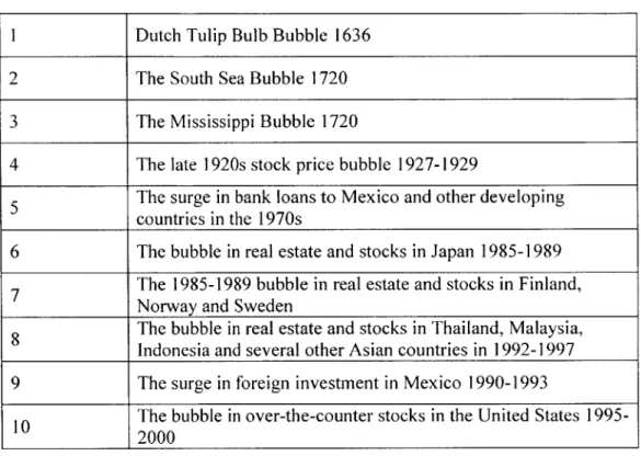
following table shows the big ten financial crises (Kindleberger, C. P. 2000).

Table 1. Big Ten Financial crises I Dutch Tulip Bulb Bubble 1636

2 The South Sea Bubble 1720 3 The Mississippi Bubble 1720

4 The late 1920s stock price bubble 1927-1929

5 The surge in bank loans to Mexico and other developing countries in the 1970s

6 The bubble in real estate and stocks in Japan 1985-1989

7 The 1985-1989 bubble in real estate and stocks in Finland, Norway and Sweden

8 The bubble in real estate and stocks in Thailand, Malaysia, Indonesia and several other Asian countries in 1992-1997 9 The surge in foreign investment in Mexico 1990-1993

10 The bubble in over-the-counter stocks in the United States 1995-2000

2.2.2 ALM at different stages in the economic cycle

Economic cycles are complex and will affect economic activities in all areas. From the basic characteristics analyzed above, many variables would affect the results of asset liability management of financial institutions. For the asset side, the variables in economic cycle, like the interest rate and security market price, would have a

return of a stock market in a certain fiscal year, the more gain the financial

institutions can get from equity class. For the liability side, the variables such as

interest rate and expected inflation rate will affect the cost of the liability. For

example, the higher expected inflation, the higher implied rates should be priced in

the insurance policy in order to attract the clients. These variables which affect the

ALM show certain distribution in different economic stages.

One whole economic cycle will experience recovery, boom, slump and recession.

Different stages have different characteristics.

In the stage of recovery, Consumer Product Index (CPI) would slightly rise, stock

prices also increase, manufacturing production expands, monetary circulation speed is

faster and the interest rate is relatively low. In this stage, the return of the asset is high

due to the prosperous capital market and the cost of liability is moderate as the CPI

expectation is not high in this stage.

When the recovery continues, the economy steps into the booming stage. CPI

accelerates the rise, stock price rising slows down; manufacturing production is still

expanding, the velocity of money is super quick, the credit of the whole economy

extends to the maximum. However, due to the general rise in prices and production

scale, money is still scarce and interest rates rise to a moderate level. Transportation,

energy, raw materials are in shortage. Housing prices are extremely high but there is

still some volume to support the price. Consumer loans expand and triangular debts

increase. Then false prosperity appears. In this stage, the return of the asset is still high because of a good capital market price. And the cost of new liability which flows in this year would be high because of the scarcity of money. These high cost

liabilities often bring negative results in the following stage.

The economy may slump when default happens and go to the stage of crisis. Goods are overproduced. There is no trade in the real estate market and housing prices

quickly drop. Stock prices depreciate. Many factories become bankrupt or are trapped into difficulty. Unemployment maintains a high level. The velocity of money is very slow and credit is stagnant. Money is very scarce while interest rates soar. This stage is the hardest time for financial institutions' ALM. In this situation, the asset return will go down and the new coming liability cost would be extremely high. The probability of squeezing is very high at this stage. So many financial institutions run out of cash in this stage and lack capital.

Then the economy comes into recession or depression stage. The overproduction continues in this stage. CPI is still declining. The capacity of manufacturing maintains an excessive rate. The business activity is decreased to a low level and the money is

also excessive. Interest rates fall to the lowest level. In the recession stage, the asset return would be low and the liability cost is also low. But the profit of the financial institution will maintain in the low level because the market players have not enough money and are cautious after the panic. If the recession stage takes a long time with a high unemployment rate, we name the serious recession, depression.

2.2.3 The economic cycle research

There is a long history of studies on the economic cycle. In 1819, Jean de Sismondi

first systematically exposited cyclic economic changes. This theory became an

important academic explanation of the 1825 crisis, which was the first obvious global

economic crisis in peaceful times. He identified the overproduction and

underconsumption before the collapse and pointed out that wealth inequality was its

reason. In 1867, Karl Marx further studied the periodic crisis in the Das Kapital.

Early study about the economic cycle focused on the political issue.

Since the economic cycle was pointed out, many studies tried to find the reasons.

Credit cycle is one of the important theories. In credit cycle theory, the increasing

weight of total debt over GDP pulls economic expansion while the shrinking of total

debt size over GDP causes recession. The persisting recession results in the

depression. This theory takes the high leverage ratio as the proximate cause of the

crisis and financial institutes which provide credit for economic activities are the

center of the economic cycle.

A primary theorist using the credit cycle to explain the cause of the economic cycle is

Irving Fisher. He created a debt deflation system to explain the depression and the

whole cycle of the economy in his classic work Blooms and Depressions and Debt

Deflation. A more recent additional theory is Financial Instability Hypothesis, which

Keen are representatives for this theory. Minsky proposed an explanation of cycles founded on fluctuations in credit, interest rates and financial frailty, called

the Financial Instability Hypothesis. In an expansion period, interest rates are low and companies easily borrow money from banks to invest. Banks are not reluctant to issue loans because expanding economic activity brings businesses increasing cash flows and therefore strongly supports their ability to pay back the loan. This process leads to firms becoming excessively indebted, so that they stop investing, and the economy goes into recession. Since then, it has been a long time since much empirical research was carried out to study the relationships between complicated business behaviors and representative indicators or ratios in view of economic cycle.

2.3 Fisher's opinion on the economic cycle

In this part, we discuss more about the Fisher's opinion on the economic cycle which we will use to construct the economic cycle in the ALM model later (Fisher, 1. 1933).

In Fisher's classic work Debt Deflation Theory of Great Depression 1933, he pointed out the dominant reason which causes recessions and depressions is

over-indebtedness at the starting point and the debt deflation follows this phenomenon soon after. He created a theory that the credit cycle makes the economic cycle and many other factors which seemingly explain the economic cycle are minor factors. This way is proved to simplify the problem of the economic cycle by deducting a huge number of correlated variables in the economic cycle.

This theory holds a view that all complex variables in the economic cycle can be narrowed down to two factors: the over-indebtedness problem, or debt deflations problem. In this theory, Fisher also incorporated that fact that debt might not be paid in real business. Fisher argued a chain reaction on how the Great Depressions

happened (nine chain reactions): over-confidence leads to over-indebtedness. Over-indebtedness would lead the debt liquidation, which results in selling off at deep discount. Then the deposit in bank system will shrink when the loans are paid off. So the circulation velocity of currency slows down. This phenomenon is accompanied by the falling of price levels and dollar depreciation. Then the net worth of assets

decreases more, accompanied by bankruptcies. In this situation, profit from

manufacturing is decreased and the worries of expected loss will appear and spread in the business world. This concern leads to reduction of output, trade and employment in real economy. These losses, bankruptcies and unemployment hurt confidence. Then these lead to hoarding and slows down the circulation velocity. All the above causes complicated disturbances in the rates of interest: the fall of the real interest rate but the rise of the real interest rate.

Fisher's theory explicates the causal relationship of the economic variables, so we can use this to simplify the parameters of the ALM model.

3. ALM Model throughout the Economic Cycle

In this part, we propose a model to simulate the asset liability management throughout the economic cycle.

We consider the asset liability management as a decision-making progress. We construct the economic cycle situation through simulating key characters of the economic cycle. We set a rule in the economic cycle to trigger the adjustment in the ALM model. In this way, the economic cycle becomes the environment of this ALM decision model.

3.1 General ALM Decision Progress

The goal of financial institutions is to maximize the profit throughout the economic cycle and to minimize the probability of bankruptcy. ALM is a tool to achieve this goal. In this part, we present a type of the decision process which will be incorporated in the ALM model.

3.1.1 ALM decision point

In ALM models, the users need to indicate how many years' impact they consider in the ALM decision which they must make now. This number of years could be considered as a planning horizon. This time horizon is then divided by sub periods.

Each sub period is one year long. In each sub period, the financial institution will receive liability. For example, for pension funds or insurance companies, the liability

they receive is premiums. For banks, the liability they get is the deposit. Then the

liability's structure such as duration is updated. At the end of the year, the return of

the asset is also updated. That is, at the end of each year, the new balance sheet is

generated. In practice, the value of asset and liability in the balance sheet is calculated

according to the accounting rules. This time point when actual annual information is

updated is considered as the point for ALM decision.

3.1.2 Decision of funding

At the decision point, financial institutions will make the decision as to whether it should raise funds or not. At this point, the gap between the values of the asset and the liability is determined. In a pension fund, this gap is measure by funding ratio,

which is defined as the ratio of the assets to its liabilities. When funding ratio is above

1, all obligated payment is able to be covered. In our ALM model, we use funding

ratio to indicate the current position risk for the financial institution and to measure its

periods as an indicator to reflect the probability of bankruptcy and help the

management of the financial institution to adjust the strategy. When the funding ratio is close to the minimum requirement, the management will seek funding and tend to invest in conservative assets. When the funding ratio is relatively high, the

management will tend to invest in risker assets. Changing the liability cost is another possible method to adjust decision progress. When the funding ratio decreases in the previous year, the management will decrease the cost of the liability. When the

management will tend to increase the cost of liability in order to expand the business size. Usually, financial institutions would set a minimum required level for the funding ratio. When the funding ratio is below the required level, financial

institutions will raise the capital to make sure that they are able to cover the liability. In the real world, the criterion of funding ratio is required by the regulators in similar forms. The insurance regulator will ask the insurers to stay solvent. The bank

regulator will ask the banks to keep capital adequacy ratio.

3.1.3 Decision of asset allocation

At the decision point, financial institutions will make the decision as to whetherit should adjust the asset allocation to maintain certain risk levels. When the actual business information is updated, the expectation for the future economic environment is also updated. Adjusting asset allocation is one of the important ways for the financial institutions to achieve high return with certain level risk. For example, financial institutions usually invest multiple asset classes to diversify the risk and they would like to maintain the asset allocation to some target asset allocation. When time passes, the asset allocation would deviate from the target allocation because of the different returns of different asset class throughout the same period. At the decision point, financial institutions have learnt this deviation of actual investment portfolio. They will make the decision to rebalance the portfolio to the original target asset

allocation or they will adjust the asset allocation strategy given the updated economic expectation.

3.1.4 Decision of liability cost

At the decision point, another way to adjust the ALM strategy is to adjust the cost of

liability. In a normal situation, the liability products sold by financial institutions are

closely related to the current prime interest rate. In the low interest level environment,

the new liability products cost is low and in the high interest level environment, the

new liability products cost is probably high. When the expected investment return is

going down, financial institutions may decrease the cost of the liability in order to

avoid the loss that happening in the future.

In determining the ALM decision, the updated information with respect to economic

cycle will be taken into account. It should be also incorporated in the future decision

making point when the new information is known.

3.2 Characteristics of ALM model

3.2.1 ALM model key factors

The first step of the ALM model is to construct a financial institute's balance sheet

which we do with asset liability management. In this balance sheet, the asset structure

and the liability structure are the most basic factors in the ALM model. Asset

allocation is reflected in the asset side of the balance sheet and brings the future cash

inflow. Asset allocation is the primary determinative reason for the return of the asset.

And for the liability side, the financial institution is concerned with the structure of the liability much as it determines the future's cash out flow. Duration is a normal way to measure the average term structure of the liability. When a new liability

product is sold, a certain amount of cash flow comes into the financial institution. And then it will invest in certain asset classes according to the asset allocation policy of the company. Simultaneously, the future out-flow with respect to this certain liability is determined. For the capital on the balance sheet, financial institutions are more concerned with the future capital funding. Based on the analysis of funding decision making, funding is a way to make sure that the asset can cover the liability.

3.2.2 Economic environment key factors

The next step is to create an environment in which the financial institution employs the ALM model. We constructed an economic cycle with the typical four stages of

recovery, boom, slump and recession. Each stage should incorporate the factors which affect the ALM model. Usually, the recovery stage is the longest stage of the economic cycle and the crisis/slumping stage is the shortest stage. In each stage, the asset return and liability cost have different distribution patterns. For example, in the recovery stage, the return of equity investment will be very high but in the boom stage, the growth of equity return will slow down.

For each year, the asset side increases or decreases and is then credited to the balance sheet at the end of the year. The change in the liability side is also credited to the

statement at that point. For each year, the movement cash flow for the new liability

happened on the last day of the fiscal year and then affects the balance sheet only

once. For each year, the balance sheet changes once on the last day of the fiscal

calendar. The exogenous cash flow is only the liability and funding cost. We do not

count the dividend payment or tax payment. The expense of the company is assumed

to be deducted in the return.

3.2.3 Employing ALM decision in the economic cycle

The purpose of this step is to put the ALM model of the financial institution into the

economic cycle to make ALM decisions. At the starting point, the financial institution

has a balance sheet at the starting point. The financial institution will employ ALM

decision-making strategy in the whole economic cycle. This decision-making strategy

is triggered by signals from the economic environment.

3.3 ALM Economic Cycle Model

3.3.1 The planning horizon of ALM

We assume the ALM model has a prediction horizon with the length of T years. We use 0 to denote the starting time of the prediction horizon, and t to denote any year within the prediction horizon, i.e. t E N and 0 5 t T. According to the above

definition, we can represent the span of any year t as [t-1, t).

3.3.2 The financial institution construction

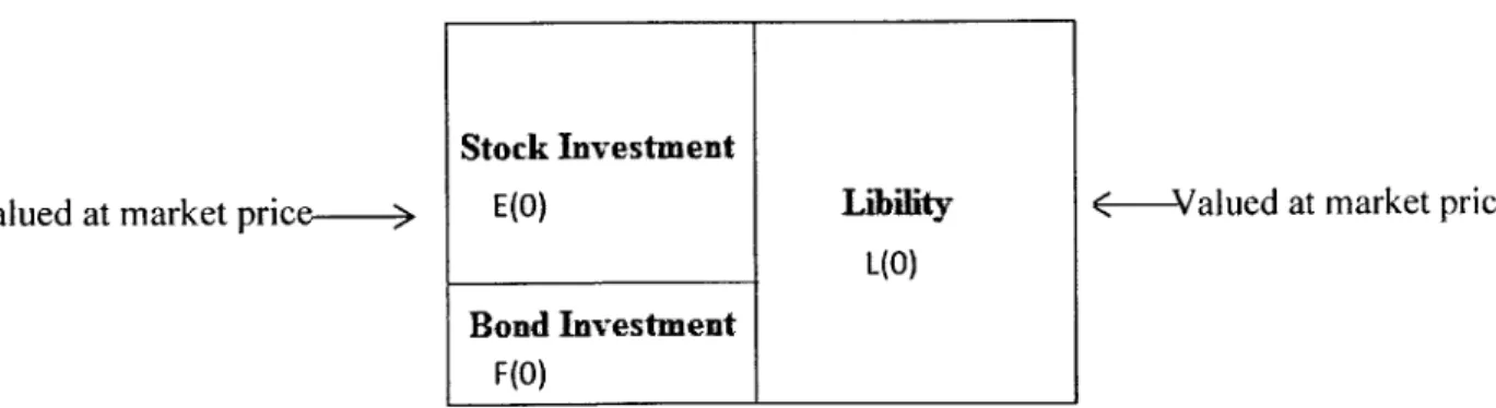
We assume the financial institution has a simple balance sheet at the starting point. We assume at the starting point the asset can cover the liability perfectly. This means we ignore the original capital of the financial institution and we are more concerned with future funding because the purpose of the model is to look forward but not to evaluate the current situation. All the items in the balance sheet are valued at market price basis, not the accounting basis because this can measure the risk more correctly.

Figure 6. Balance Sheet at Starting Point (t = 0)

Valued at market price > (-Valued at market price

Stock Investment

E(O) Libility

L(O)

Bond Investment F(O)

We use

S(t)

to denote the market value of the whole asset at time t. For the asset side,

we assume it has an asset portfolio with only two asset classes: investment grade

fixed income and large cap equity. We use E(t) to denote the market value of stock

investment at year t and F(t) to denote the market value of bond investment.

In each year t, the financial institution will get the cash flows from its business. We

use C(t) to denote the net cash flows from its business at time t. We assume only the

net liability can affect C(t). For example, the insurance company gets 100 million

from premium and pays 80 million for its client at some certain year. At this point,

the net cash flow C(t) is 20 million. We use Fu(t) to denote the cash flow from the

new contribution of the capital at time t.

For the net cash flow C(t), we assume it is only increased by the cash flow from new

liability and decreased by paying the liability holder. We use Lin(t) to denote the new

liability by the time t and we use Lout(t) to denote the liability that is paid to the

liability holder by the time t. So we get:

C(t)

=

_{Lin(t) +Lout(t) where Lout(t) <}

_o

₍₁₎

Once the net cash flow from liability (C(t)) or from the funding (Fu(t)) flow into the

financial institution, it will be invested to the same asset class in the portfolio . So we

use the t- to denote the time before the adjustment at time t. So we get the

S(t) = E(t-) + F(t-) + C(t) + Fu(t)

S(t) = E(t) + F(t)

(2)

(3)

At each time t, the financial institution can know the change on the balance sheet. For the asset side, we use the r(t) to denote the return of equity by the time t and we use the s1(t) to denote the return of fixed income by the time t. As a result we will get:

E(t) = (r(t) + 1) x E(t - 1)

F(t) = (s1(t) + 1) x F(t - 1)

(4)

(5)

For the liability side, we use L(t) to denote the Value of the liability by the time t. We also use the s2 to denote the value change of liability by the time t.

L(t) = (s2(t) + 1) x L(t - 1) (6)

We use Lout to denote the cash flow, that comes out in certain period t and use Lin to denote the cash flow that comes in certain period t. We use i(t) to denote the interest rate at time t and we use g(t) to denote the GDP growth rate at time t. We define Lin as following:

We also assume that at starting point t = 0, the all liability should evenly be paid off

in P years, so we will get:

Lout(1) =

L(0)

+

(8)

When the new liability Li,(]) at time t =1 comes in, we assume that cash will be paid

to the creditors evenly in following P years. So for t

=

2 we will get

Lout(2)

=

L(0)

+

1

+ Lin(1)

p

(9)

With respect to certain Lin(t), the amount will be amortized fully within P years.

Because the liability is valued as the market value, so the cost of the liability is priced

in the growth rate of liability return.

3.3.3 The decision process

At each time t, after the financial institution reevaluates the market value of the portfolio and counts the impact of the cash flow, the management is allowed to make a decision based on the actual information. Given the previous year's returns, and the expected return of the future, the management will adjust the strategy for the

following year. For example, when the liability value is much higher than the asset

value, the financial institution may tend to find some contribution to the equity to

make up the shortage.

The decision's goal is to maximize the benefit and control the bankruptcy and liquidity risks. So we assume the funding ratio r should meet the minimum requirementa. We simplify the decision process to set a trigger to compensate the fund to make sure the asset coverage over the liability.

At the decision-making point t, we compare updated asset value and liability value. When the asset could not cover the liability, we will raise the funding. We assume the minimum capital requirement is 1. The amount of the funding is a multiple of 1.

We assume the multiple is a. So the mathematical expression is shown as following:

if E(t) + F(t) > 1, Fu(t) = 0

if E(t-) + F(t-) < L(t), Fu = a x 1 (10)

After the funding is determined, the new cash flow both from funding and net liability product should be invested in certain assets.

We assume the financial institution employs the asset allocation strategy to invest y percentage of total asset in large cap equity and (1 - y) percentage of investment

grade bond. So y is the target asset allocation for the equity investment and 1- y is the target asset allocation for the fixed income. So at starting point:

F(O)

E(O)+F(o)

The new cash flow from the funding and liability products comes into the financial institution at the time, the financial institution invests incremental cash flow to the same asset class at the same ratio at the original point. We use the E(t) to denote the large equity value after the reallocation of the new cash flow at time t while E(t~) means the large equity value before considering the new cash flow at time t. In the same way, we use F(t) denote to the large equity value after the reallocation of the new cash flow at time t while F(t-) means the large equity value before considering the new cash flow at time t.

At the decision point t, the financial institution also checks the existing portfolio asset allocation. As time passed the financial institution will make the decision for the rebalance of the portfolio to maintain a certain level of risk.

As we discussed above, the interest is the most direct ratio to reflect the credit situation in the different economic cycle stage. So we set a trigger in the economic cycle to rebalance the portfolio to incorporate the interest rate.

We use the i* to denote the trigger interest rate, and we use the i to denote the interest rate at time t, i* will change in different economic cycle stage. So we get:

If i < i*, the financial institution will keep the asset allocation at time t-1

E(t) = E(t-) + (C(t) + Fu(t)) x y

F(t) = F(t-) + (C(t) + Fu(t)) x (1 - y)

(13)

(14)

If i > i*, the financial institution will rebalance the asset allocation and we get:

E(t) = (E(t-) + C(t) + Fu(t)) x y

F(t) = (F(t~) + C(t) + Fu(t)) x (1 - y)

(15)

(16)

3.4 Simulation

3.4.1 Flow chart of ALM model

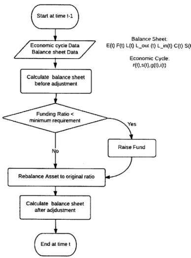
We use Matlab to simulate the model. The flowchart of the model at time t is as following:

Figure 7. Flowchart at time t

Balance Sheet:

E(t) F(t) L(t) Lout (t) Lin(t) C(t) S(t)

Economic Cycle:

r(t),s(t),g(t),i(t)

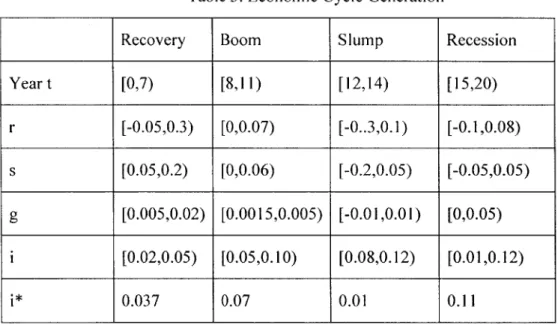
3.4.2 Scenario Generation

To simulate the ALM model in the economic cycle, we assign the value of the

let the Matlab generate randomly given the limitation of Table 3 with even

distribution.

Table 2. Time Horizon Generation

Table 3. Economic Cycle Generation

Recovery Boom Slump Recession

Year t [0,7) [8,11) [12,14) [15,20) r [-0.05,0.3) [0,0.07) [-0..3,0.1) [-0.1,0.08) s [0.05,0.2) [0,0.06) [-0.2,0.05) [-0.05,0.05) g [0.005,0.02) [0.0015,0.005) [-0.01,0.01) [0,0.05) i [0.02,0.05) [0.05,0.10) [0.08,0.12) [0.01,0.12) i* 0.037 0.07 0.01 0.11

Table 4. Related Constant

a 1.5 p' 50000 I 15 E(0) 20 F(0) 80 L(0) 100

3.4.3

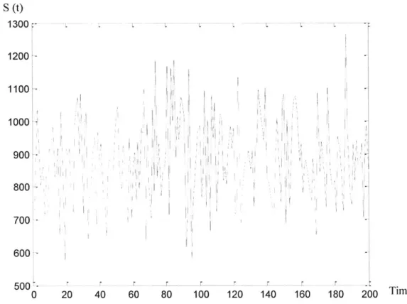
Simulation Result

We run the model given above information 200 times. The average number of times

for fund raising is 9.36 in 20 years and the average terminal asset value S(20) is

884.7597 if we assume its asset value S(0) starts with 100'.

Figure 8. Terminal Asset Value S(20)

S

Figure 9. Times for raising fund -10 9.5 9 8.5--8 7 - r r r r 0 20 40 60 80 r7 - f - r r 100 120 140 160 180

3.5 Conclusion

We simulate how a financial institution makes decisions throughout economic cycles.

In order to simulate, we established a model to reflect how the economic cycle affects

the financial institution's value by using the economic relationship. Then we set up

the decision-making progress according to economic cycle's triggers. Finally we

observe the changes of system in a time horizon.

'I! I III I I I II II II II 7.5 K I -~ 200 Times 10.5F-11 1 1

Appendix

Sample Code for Matlab Simulation

T=20;

economic=[-]; % example 4 different distribution: economic=[-]

% example r,s,g,1,iDecision scale and distribution rLeft=[-]; rRight=[-]; sLeft=[-]; sRight=[-] gLeft=[-]; gRight=[-]; iLeft=[-]; iRight=[-]; iDecision=[-];

% example starting balance sheet:

constLin=50000; EO=20; FO=80; LO=100; constFu=15; multiplerFu=1.5; S_all=[]; E_all=[]; F_all=[]; C_all=[]; Funumber_all=[]; iDecisionnumber all=[]; for execution=1:200 Lin=[]; Loutcomponent=[]; Loutcomponent check=[]; Funumber=0; iDecisionnumber=O; Loutcomponent=[LO/beta]; E=EO;F=FO; L=LO; for t=1:T for i=1:length(economic)

if economic(i)<t && t<=economic(i+1) period=i; end end r=rLeft(period)+(rRight(period)-rLeft(period)).*rand(1,1); E_before=(1+r)*E; s=sLeft(period)+(sRight(period)-sLeft(period)).*rand(1,1); F_before=(1+s)*F; i1=iLeft(period)+(iRight(period)-iLeft(period)).*rand(1,1); g=gLeft(period)+(gRight(period)-gLeft(period)).*rand(1,1);

Lout_component=[Loutcomponent Lin/beta]; % from 0 to t-1 Lin=constLin*il*g; %Lin at the current time t

for i=1:length(Lout-component) if Loutcomponent(i)-(t-i)*Loutcomponent(i)/beta>o Loutcomponent check(i)=1; else Loutcomponent check(i)=O; end end

Lout=sum(Lout component.*Lout component check); C=Lin+Lout; i2=i Left(period)+(iRight(period)-iLeft(period)).*rand(1,1); L=(1+i2)*L+C; if L-(E_before+F_before)>constFu Fu=constFu*multiplerFu; Funumber=Funumber+1; else Fu=O; end

if iDecision(period)<i %&& kiiRight E=(E_before+Fbefore+C+Fu)*EO/(EO+FO); F=(E_before+Fbefore+C+Fu)*FO/(EO+FO); iDecisionnumber=iDecisionnumber+1; else E=E before+(C+Fu)*E/(EO+FO); F=F before+(C+Fu)*FO/(EO+FO); end end S=E+F+C+Fu; S_all=[Sall S]; E_all=[Eall El; F_all=[Fall F]; C_all=[F_all C];

Funumber all=[Fu_numberall Funumber];

iDecisionnumber_all=[iDecisionnumber-all iDecision-number]; end sum(Sall)/200 sum(Fu_numberall)/200 figure; plot(Sall); figure; plot(Fu_numberall); ylim([7 10.5])

References

Danielsson, J. et al. (2011) Balance Sheet Capacity and Endogenous Risk. Working Paper, p.2. Available at: http://www.princeton.edu/~hsshin/www/balancesheetcapacity.pdf

[Accessed: 1 April 2013].

Zenios, S. A., & Ziemba, W. T. (2006). Handbook of asset and liability management. Volume 1, Theory and Methodology. Amsterdam, Elsevier North Holland, P4-5.

Zenios, S. A., & Ziemba, W. T. (2006). Handbook of asset and liability management. Volume 1, Theory and Methodology. Amsterdam, Elsevier North Holland, P18-21.

Honkapohja, S. (2009) Financial crises: characteristics and crisis management. [online] Available at:

http://www.actuaries.org/ASTIN/Colloquia/Helsinki/Presentations/Honkapohja.pdf [Accessed: 11 Apr 2013].

Kindleberger, C. P. (2000). Manias, panics, and crashes: a history offinancial crises. New York, Wiley.

Fisher, 1. (1933) The Debt-Deflation Theory of Great Depressions. Econometrica,

Available at: http://fraser.stlouisfed.org/docs/meltzer/fisdeb33.pdf [Accessed: April 1, 2013]. Ziemba, W. T., & Mulvey, J. M. (1998). Worldwide asset and liability modeling.

Cambridge, United Kingdom, Cambridge University Press.

Carifio, D. and Kent, T. (1994) The Russell-Yasuda Kasai Model: An Asset/Liability Model for a Japanese Insurance Company Using Multistage Stochastic

Programming. Interfaces, 24 (1), p.2 9_-4 9_.