HAL Id: hal-01564899
https://hal.archives-ouvertes.fr/hal-01564899
Submitted on 19 Jul 2017
HAL is a multi-disciplinary open access
archive for the deposit and dissemination of
sci-entific research documents, whether they are
pub-lished or not. The documents may come from
L’archive ouverte pluridisciplinaire HAL, est
destinée au dépôt et à la diffusion de documents
scientifiques de niveau recherche, publiés ou non,
émanant des établissements d’enseignement et de
Improving the Spatial Solution of Electrocardiographic
Imaging: A New Regularization Parameter Choice
Technique for the Tikhonov Method
Judit Chamorro-Servent, Rémi Dubois, Mark Potse, Yves Coudière
To cite this version:
Judit Chamorro-Servent, Rémi Dubois, Mark Potse, Yves Coudière. Improving the Spatial Solution of
Electrocardiographic Imaging: A New Regularization Parameter Choice Technique for the Tikhonov
Method. 9th International Conference on Functional Imaging and Modelling of the Heart - FIMH
2017, Jun 2017, Toronto, Canada. pp.289-300, �10.1007/978-3-319-59448-4_28�. �hal-01564899�
Improving the spatial solution of electrocardiographic
imaging: A new regularization parameter choice
technique for the Tikhonov method
Judit Chamorro-Servent 1,2,3,* (0000-0002-5722-0499), Rémi Dubois1,4,5, Mark Potse1,2,3 (0000-0003-4166-2687), Yves Coudière1,2,3
1IHU Liryc, Electrophysiology and Heart Modeling Institute, foundation Bordeaux Université, Pessac-Bordeaux, France
2CARMEN Research Team, INRIA, Bordeaux, France
3Univ. Bordeaux, IMB, UMR 5251, CNRS, INP-Bordeaux, Talence, France 4Univ. Bordeaux, CRCTB, U1045, Bordeaux, France
5INSERM, CRCTB, U1045, Bordeaux, France [email protected]
Abstract. The electrocardiographic imaging (ECGI) inverse problem is highly
ill-posed and regularization is needed to stabilize the problem and to provide a unique solution. When Tikhonov regularization is used, choosing the regulariza-tion parameter is a challenging problem. Mathematically, a suitable value for this parameter needs to fulfill the Discrete Picard Condition (DPC). In this study, we propose two new methods to choose the regularization parameter for ECGI with the Tikhonov method: i) a new automatic technique based on the DPC, which we named ADPC, and ii) the U-curve method, introduced in other fields for cases where the well-known L-curve method fails or provides an over-regularized so-lution, and not tested yet in ECGI. We calculated the Tikhonov solution with the ADPC and U-curve parameters for in-silico data, and we compared them with the solution obtained with other automatic regularization choice methods widely used for the ECGI problem (CRESO and L-curve). ADPC provided a better cor-relation coefficient of the potentials in time and of the activation time (AT) maps, while less error was present in most of the cases compared to the other methods. Furthermore, we found that for in-silico spiral wave data, the L-curve method over-regularized the solution and the AT maps could not be solved for some of these cases. U-curve and ADPC provided the best solutions in these last cases.
Keywords: inverse problem; regularization; electrocardiographic imaging;
1
Introduction
During the past decades, much progress has been made in solving the inverse problem of electrocardiography [1-7]. However, despite all the success of non-invasive electro-cardiographic imaging (ECGI), the understanding and treatment of many cardiac dis-eases is not feasible yet without an improvement of the inverse problem solution [8]. Solution of the ‘inverse problem’ depends on the ‘forward problem’, i.e. on specifica-tion of the relaspecifica-tionship between potential sources on the cardiac surface, Φ𝐸𝐸, and the body surface measured potentials, Φ𝑇𝑇.
The inverse problem (finding Φ = ΦE at epicardial surface 𝛤𝛤𝐸𝐸) is innately ill-posed. That means that is extremely sensible to: i) noise on the measured potentials, ii) uncer-tainty in the location of measurement sites with respect to the surface on which the sources are distributed, iii) errors of segmentation of the geometries, and iv) influence of cardiac motion.
Regularization incorporates additional knowledge in the inverse problem by apply-ing constraints to the solution, to stabilize the problem yieldapply-ing realistic and unique results. When regularization is applied, the weight of the constraints (regularization parameter) has to be determined to find a balance between solutions purely based on the body-surface potentials and solutions that are constrained too strictly. While the former may be severely distorted by ill-posedness, the latter may have too much bias. Given the ill-posedness, the regularization parameter choice has an important influence on the solution [8].
In this study we focused on the two-norm Tikhonov regularization technique for the method of fundamental solution (MFS), an homogeneous meshless method adapted to ECGI by Wang and Rudy [9,10]. Specifically, we will focus on the choice of the regu-larization parameter. In many implementations, the Tikhonov reguregu-larization problem is solved by manually selecting the regularization parameter 𝛼𝛼. This is done using a se-quence of regularization parameters and selecting the value that gives the best results, as judged by the user. Obviously, the procedure is subjective and time consuming. To overcome this problem, several automatic methods for selecting regularization param-eters have been suggested over the years. These include: i) Strategies based on the cal-culation of the variance of the solution, which requires prior knowledge of the noise, ii) Strategies that do not need a priori information. For ECGI, we are interested in the latter.
Regarding the second group (ii) of automatic methods previously used in the MFS ECGI literature [9,10], the regularization parameter is obtained by using the mean of the regularization parameters provided by the Composite Residual and Smoothing Opera-tor (CRESO) technique [10]. The CRESO method has been found to perform compara-bly to the “optimal” regularization parameter that provides the minimum root-mean-square error (RMSE) between the computed epicardial potentials (Φ𝐸𝐸) and the meas-ured ones [10]. When other numerical methods, such as the Boundary Element method (BEM), were used to solve the ECGI problem, the L-curve criterion has been highly used by the community to find the regularization parameter [8, 11].
While the efficacy of the CRESO and L-curve methods has been proven in the wide inverse problems literature [8-16], finding an automatic regularization parameter for
Tikhonov regularization that is suitable for all ill-posed inverse problems is a challeng-ing problem [12, 15] and CRESO and L-curve may over-regularize the solution or fail for some cases. This is especially important when we deal with medical problems such as cardiac pathologies, where different pathologies may need different regularization.
For this reason, the overarching goal of this paper is to show the feasibility of the U-curve method [17-18], not used yet in cardiac inverse problems, after our knowledge; and to develop a new automatic method, ADPC, based on the Discrete Picard Condition (DPC), a mathematical condition that any suitable regularization parameter for Tikhonov regularization must fulfill [12].
2
Methods
2.1 Method of fundamental solutions and Tikhonov regularization
MFS is a homogeneous meshless approach that was adapted to ECGI to overcome some of the issues of the classical meshes-based methods [9-10]. MFS does not need the topological relations between nodes and so completely avoids disadvantages of ac-curacy degradation and complexity augmentation frequently encountered in classical numerical methods because of remeshing. Thus it avoids, negative effects introduced by errors in the segmentation process and/or singularities in the boundaries.
In the MFS, the potentials are expressed as a linear combination of Laplace funda-mental solution over a discrete set of virtual source points (Dirac masses) placed outside of the domain of interest, Ω, where Ω is the volume conductor enclosed by the epicar-dial surface 𝛤𝛤𝐸𝐸 and the body surface, 𝛤𝛤𝑇𝑇. Specifically the potential Φ for 𝑥𝑥 ∈ Ω is sought as
Φ(𝑥𝑥) = 𝑎𝑎0+ ∑𝑁𝑁𝑗𝑗=1𝑆𝑆 𝑓𝑓�𝑥𝑥 − 𝑦𝑦𝑗𝑗�𝑎𝑎𝑗𝑗, (1)
where the �𝑦𝑦𝑗𝑗�
𝑗𝑗=1..𝑁𝑁𝑆𝑆 are the 𝑁𝑁𝑆𝑆 locations of the sources �𝑦𝑦𝑗𝑗∉ Ω�, and the �𝑎𝑎𝑗𝑗�𝑗𝑗=1..𝑁𝑁𝑆𝑆 are their coefficients. Here, 𝑓𝑓 stands for the fundamental solution to the Laplace equa-tion, 𝑓𝑓(𝑟𝑟) = 1
4𝜋𝜋 1
|𝑟𝑟| where 𝑟𝑟 is the 3D Euclidean distance between point 𝑥𝑥 and virtual
source 𝑦𝑦. After discretization on collocation points on 𝛤𝛤𝑇𝑇, and fixed number 𝑁𝑁𝑆𝑆 of source locations [9], this formulation yields a linear system of equations with matrix system 𝑀𝑀: 𝑀𝑀 = ⎝ ⎜ ⎜ ⎜ ⎛ 1 𝑓𝑓(𝑟𝑟11) ⋯ 𝑓𝑓�𝑟𝑟1𝑁𝑁𝑆𝑆� ⋮ ⋱ ⋮ 1 𝑓𝑓�𝑟𝑟𝑁𝑁𝑇𝑇1� ⋯ 𝑓𝑓�𝑟𝑟𝑁𝑁𝑇𝑇𝑁𝑁𝑆𝑆� 0 𝜕𝜕𝑛𝑛1𝑓𝑓(𝑟𝑟11) ⋯ 𝜕𝜕𝑛𝑛1𝑓𝑓�𝑟𝑟1𝑁𝑁𝑆𝑆� ⋮ ⋱ ⋮ 0 𝜕𝜕𝑛𝑛𝑁𝑁𝑇𝑇𝑓𝑓�𝑟𝑟𝑁𝑁𝑇𝑇1� ⋯ 𝜕𝜕𝑛𝑛𝑁𝑁𝑇𝑇𝑓𝑓�𝑟𝑟𝑁𝑁𝑇𝑇𝑁𝑁𝑆𝑆�⎠ ⎟ ⎟ ⎟ ⎞ , where 𝑟𝑟𝑖𝑖𝑗𝑗= 𝑥𝑥𝑖𝑖− 𝑦𝑦𝑗𝑗, 𝑥𝑥𝑖𝑖∈ 𝛤𝛤𝑇𝑇 and�𝑦𝑦𝑗𝑗�
𝑗𝑗=1..𝑁𝑁𝑆𝑆, 𝑦𝑦𝑗𝑗∉ Ω. Hence, homogeneous Neumann conditions (no flux conditions,𝜕𝜕𝑛𝑛Φ = 0) and Dirichlet conditions (Φ = Φ𝑇𝑇, where
Φ𝑇𝑇 are the potentials acquired on the torso) on 𝛤𝛤𝑇𝑇 are considered in an apparently
equivalent manner in the standard MFS described in [9]. Therefore, only the sources coefficients are unknown, resulting in a quadratic minimizing problem (Tikhonov reg-ularization problem), find the sources coefficients 𝑎𝑎 = �𝑎𝑎0, 𝑎𝑎1, ⋯ , 𝑎𝑎𝑁𝑁𝑆𝑆�𝑇𝑇𝜖𝜖ℝ1+𝑁𝑁𝑠𝑠 that minimize
𝐽𝐽(𝑎𝑎, 𝛼𝛼) = ‖M𝑎𝑎 − b‖2+ 𝛼𝛼‖𝑎𝑎‖2 (2)
where 𝑏𝑏 = �Φ𝑇𝑇∗
0 � is a 2𝑁𝑁𝑇𝑇𝑥𝑥1 vector, given some potentials Φ𝑇𝑇∗ = (Φ𝑖𝑖∗)𝑖𝑖=1,⋯,𝑁𝑁𝑇𝑇 rec-orded on 𝑁𝑁𝑇𝑇 torso electrodes, and 𝛼𝛼 > 0 is the Tikhonov regularization parameter. Note that the first term ‖M𝑎𝑎 − b‖2 measures the goodness-of-fit, i.e., how well the un-known sources coefficients 𝑎𝑎 predicts the given boundary conditions at body surface. The second term ‖𝑎𝑎‖2 measures the regularity of the sources coefficients 𝑎𝑎. It sup-presses (most of) its large noise components by controlling its norm (since the naïve solution is dominated by high-frequency components with large amplitudes). The bal-ance between both terms is controlled by the regularization parameter,𝛼𝛼.
Once solved (2) and found the source coefficients 𝑎𝑎 = �𝑎𝑎0, 𝑎𝑎1, ⋯ , 𝑎𝑎𝑁𝑁𝑆𝑆�𝑇𝑇𝜖𝜖ℝ1+𝑁𝑁𝑠𝑠, the ΦE are found by using (1) for 𝑥𝑥 ∈ 𝛤𝛤𝐸𝐸 and �𝑦𝑦𝑗𝑗�𝑖𝑖=1..𝑁𝑁𝑆𝑆, 𝑦𝑦𝑗𝑗 ∉ Ω.
2.2 Discrete Picard Condition
Instead of the condition number of the matrix of a linear system, the rate of decrease of the singular values (SVs) is a better indication of the conditioning of the problem [12, 13]. Furthermore, the Discrete Picard Condition (DPC) [12] provides an objective as-sessment of the ill-posedness of the entire problem relating the matrix information (by means of the SVs) with the measurements [12].
The Tikhonov solution can be obtained by equalling the gradient of (2) to zero: 𝛻𝛻𝐽𝐽𝑎𝑎(𝑎𝑎, 𝛼𝛼) = 𝛻𝛻((𝑀𝑀𝑎𝑎 − 𝑏𝑏)𝑇𝑇(𝑀𝑀𝑎𝑎 − 𝑏𝑏) + 𝛼𝛼𝐼𝐼𝑎𝑎𝑇𝑇𝑎𝑎) = (𝑀𝑀𝑇𝑇𝑀𝑀)𝑎𝑎 − 𝑀𝑀𝑇𝑇𝑏𝑏+𝛼𝛼2𝐼𝐼𝑎𝑎 = 0 , and
𝑎𝑎𝛼𝛼 = (𝑀𝑀𝑇𝑇𝑀𝑀 + 𝛼𝛼2𝐼𝐼)−1𝑀𝑀𝑇𝑇𝑏𝑏.
Then, by decomposing the forward matrix of the MFS in terms of SV decomposition (𝑀𝑀 = 𝑈𝑈𝑈𝑈𝑉𝑉𝑇𝑇) and writing 𝐼𝐼 = 𝑉𝑉𝑉𝑉𝑇𝑇, 𝑎𝑎𝛼𝛼 = ∑ 𝜎𝜎𝜎𝜎𝑖𝑖 𝑖𝑖2+𝛼𝛼2𝑢𝑢𝑖𝑖 𝑇𝑇𝑏𝑏𝑣𝑣 𝑖𝑖= ∑ 𝜎𝜎𝑖𝑖 2 𝜎𝜎𝑖𝑖2+𝛼𝛼2 𝑢𝑢𝑖𝑖𝑇𝑇𝑏𝑏 𝜎𝜎𝑖𝑖 𝑣𝑣𝑖𝑖 min �2∗𝑁𝑁𝑇𝑇,𝑁𝑁𝑆𝑆+1� 𝑖𝑖=1 min �2∗𝑁𝑁𝑇𝑇,𝑁𝑁𝑆𝑆+1� 𝑖𝑖=1 (3)
where 𝜎𝜎𝑖𝑖 are the SVs in descending order, 𝜎𝜎1≥ ⋯ ≥ 𝜎𝜎min �2∗𝑁𝑁
𝑇𝑇,𝑁𝑁𝑆𝑆+1�(the elements of the diagonal matrix 𝑈𝑈).
The DPC is satisfied if the data space coefficients |𝑢𝑢𝑖𝑖𝑇𝑇𝑏𝑏|, on average, decay to zero faster than the respective 𝜎𝜎𝑖𝑖’s. The representation of |𝑢𝑢𝑖𝑖𝑇𝑇𝑏𝑏|, 𝜎𝜎𝑖𝑖, and the respective quo-tient in a same plot in logarithmic scale is known as a Picard plot.
In ill-posed problems, such as ECGI, there may be a point where the data become dominated by errors and the DPC fails. In other words, for larger values of the index 𝑖𝑖
the solution coefficients�𝑢𝑢𝑖𝑖𝑇𝑇𝑏𝑏�
𝜎𝜎𝑖𝑖 start to increase and the computed solutions (3) are com-pletely dominated by the SVD coefficients corresponding to the smallest SVs. In these cases, to compute a satisfactory solution by means of Tikhonov regularization, the DPC has to be fulfilled [12, 18]. That is, the 𝜎𝜎𝑖𝑖 above the regularization parameter 𝛼𝛼 (useful SVs) must decay to zero slower than the corresponding right hand side coeffi-cients, | 𝑢𝑢𝑖𝑖𝑇𝑇𝑏𝑏|. The DPC determines how well the regularized solution approximates the unknown, exact solution.
2.3 Existent regularization parameter choice techniques
Composite Residual and Smoothing Operator (CRESO)
CRESO was developed by Colli-Franzone et al. [14]. The method was presented as an empirical heuristic but has become widely accepted as the preferred method of param-eter estimation in a large class of ill-posed bioelectric inverse problems [15]. The CRESO method chooses that parameter value which generates the first local maximum of the difference between the derivative of the constraint term and the derivative of the residual term
𝐶𝐶(𝛼𝛼) = �𝑑𝑑(𝛼𝛼𝑑𝑑2)(𝛼𝛼2‖𝑥𝑥(𝛼𝛼)‖2) −
𝑑𝑑
𝑑𝑑(𝛼𝛼2)‖𝑀𝑀𝑥𝑥(𝛼𝛼) − 𝑏𝑏‖2, 𝛼𝛼 > 0� (4)
L-curve
The best-known method for estimating a value for the regularization parameter is de-fined in terms of the L-curve [15, 16]
𝐿𝐿(𝛼𝛼) = {(‖𝑀𝑀𝑥𝑥(𝛼𝛼) − 𝑏𝑏‖, ‖𝑥𝑥(𝛼𝛼)‖), 𝛼𝛼 > 0} (5) To choose the L-curve regularization parameter we used the criterion proposed by Han-sen and O’Leary [16], where the optimal 𝛼𝛼-value corresponds to the point on the log-log plot of the L-curve possessing maximum curvature.
U-curve
The U-curve method was proposed by Krawczyck-Stando and Rudnicki [17]. The U-curve is the plot of the sum of the inverse of the regularized solution norm ‖𝑥𝑥(𝛼𝛼)‖ and the corresponding residual error norm ‖𝑀𝑀𝑥𝑥(𝛼𝛼) − 𝑏𝑏‖, for 𝛼𝛼 > 0 on a log-log scale
𝑈𝑈(𝛼𝛼) =
‖𝑀𝑀𝑀𝑀(𝛼𝛼)−𝑏𝑏‖1 2+
1‖𝑀𝑀(𝛼𝛼)‖2 (6)
The U-curve is a U-shaped function, where the sides of the curve correspond to regu-larization parameters for which either the solution norm or the residual norm dominates. The optimum regularization value is the value for which the U-curve has a minimum. U-curve is computationally efficient since it provides an a priori interval where to find this minimum [17-18]. Furthermore, while its feasibility has not been tested yet for ECGI, it has been shown to perform well for some numerical and biomedical problems when the L-curve failed or gave an over-regularized solution [17-18].
2.4 ADPC: A new regularization parameter choice method
As cited before, a suitable regularization parameter 𝛼𝛼 for Tikhonov regularization must fulfill the DPC. This means that the 𝜎𝜎𝑖𝑖 above the suitable 𝛼𝛼 must decay to zero slower than the corresponding |𝑢𝑢𝑖𝑖𝑇𝑇𝑏𝑏|, in order to prevent the computed Tikhonov solutions (3) from being completely dominated by the SVD coefficients corresponding to the small-est SVs. Therefore, we performed an automatic regularization parameter choice method based on this condition as follows:
1. We calculate the singular value decomposition of the MFS matrix, 𝑀𝑀, to obtain the left singular vectors (𝑢𝑢𝑖𝑖) and the singular values (𝜎𝜎𝑖𝑖).
2. For each instant of time, 𝑡𝑡𝑘𝑘 (𝑚𝑚𝑚𝑚), we compute �𝑢𝑢𝑖𝑖𝑇𝑇𝑏𝑏𝑡𝑡𝑘𝑘� and we fit the log (�𝑢𝑢𝑖𝑖𝑇𝑇𝑏𝑏𝑡𝑡𝑘𝑘� ) by a polynomial 𝑝𝑝�𝑖𝑖, log ��𝑢𝑢𝑖𝑖𝑇𝑇𝑏𝑏𝑡𝑡𝑘𝑘�� �
𝑡𝑡𝑘𝑘 of degree from 5 to 7. Therefore, we have: 𝑝𝑝𝑡𝑡1,⋯,𝑝𝑝𝑡𝑡𝑁𝑁𝑡𝑡 polynomials, one for each instant 𝑡𝑡𝑘𝑘, 𝑘𝑘 = 1, ⋯ , 𝑁𝑁𝑡𝑡 instants of time. 3. For each 𝑝𝑝𝑡𝑡𝑘𝑘, we find: 𝛼𝛼𝑡𝑡𝑘𝑘= 𝜎𝜎𝑚𝑚𝑎𝑎𝑀𝑀{𝑖𝑖}, such that log(𝜎𝜎𝑖𝑖) ≥ 𝑝𝑝𝑡𝑡𝑘𝑘, with 𝜎𝜎𝑖𝑖 in
descend-ing order.
4. The ADPC regularization parameter is: 𝛼𝛼 = median�𝛼𝛼𝑡𝑡𝑘𝑘�.
Note that step 2 and 3 of this algorithm are empirically choosing the lower limit that any suitable Tikhonov regularization parameter can achieve to still fulfill the DPC. Both steps are looking for the last index 𝑖𝑖 before the SVD coefficients (corresponding to the smallest SVs) start to dominate the solution. That means, before log(𝜎𝜎𝑖𝑖) starts to be smaller than log (�𝑢𝑢𝑖𝑖𝑇𝑇𝑏𝑏𝑡𝑡𝑘𝑘� ). The fitting of the log (�𝑢𝑢𝑖𝑖𝑇𝑇𝑏𝑏𝑡𝑡𝑘𝑘� ) by a polynomial is done to simplify the search for a suitable index 𝑖𝑖. Since the behavior of the SVs of ECGI MFS problem and the fact that ADPC parameter choice is based on the necessary DPC, our algorithm provides a suitable regularization parameter.
2.5 Simulated data
To test the effect of the new regularization parameter choice method and to compare with previous ones, eight different activation patterns (1 single site pacing in the right ventricular (RV) free wall, 1 single site pacing in the left ventricular (LV) lateral endo-cardial wall, 1 single site pacing in the LV mid wall, 1 single pacing site in the LV lateral epi and 4 single spiral waves) were simulated [19]. Propagating activation was simulated with a monodomain reaction-diffusion model in a realistic 3D model of the human ventricles, with transmembrane ionic currents computed with the Ten Tusscher et al. model for the human ventricular myocyte [20]. The transmembrane currents from the monodomain problem were used to compute the extracellular potential distribution throughout the torso by solving a static bidomain problem in a heterogeneous, aniso-tropic torso model at 1mm resolution [21]. The torso model used had heterogeneous conductivity, with anisotropic skeletal muscle, lungs, and intracavitary blood. The heart model consisted of left and right ventricles, with a 0.2 mm spatial resolution, and an anisotropic conduction derived from rule-based fiber orientation. Cardiac and thoracic
anatomy was based on MRI data. The simulations provide the theoretical, in-silico Φ𝑇𝑇 and Φ𝐸𝐸 every 1ms.
2.6 Analysis of the reconstructed potentials and activations time maps: Statistical approach
Once reconstructed the potentials on the epicardium, correlations coefficients (CC) and root mean square errors (RMSE) [12], and relative errors (𝑅𝑅𝑅𝑅 = �Φ𝐸𝐸− Φ� �/‖Φ𝐸𝐸 𝐸𝐸‖, where Φ𝐸𝐸 are the simulated potentials and Φ� the reconstructed ones), were computed 𝐸𝐸 through time. Thus, we compared the reconstructed potentials on the epicardium against the simulated ones. Afterwards, we calculated the three quartiles of the resulting CCs, RMSEs and REs, (Median [1st quartile, 3rd quartile]).
Similarly, we calculated the activation time (AT) maps and the respective CCs and REs (Median, [min, max]).
3
Results
3.1 Ill-posedness and Discrete Picard Condition
The DPC condition allows us to investigate the behavior of the SVD coefficients |𝑢𝑢𝑖𝑖𝑇𝑇𝑏𝑏| (of the right hand side) and �𝑢𝑢𝑖𝑖𝑇𝑇𝑏𝑏�
𝜎𝜎𝑖𝑖 (of the solution (3)). A logarithmic plot of these coef-ficients, together with the respective SVs, 𝜎𝜎𝑖𝑖 (also in logarithmic scale), is often re-ferred to as DPC plot [12]. Given 𝜎𝜎1≥ ⋯ ≥ 𝜎𝜎min �2∗𝑁𝑁𝑇𝑇,𝑁𝑁𝑆𝑆+1� , lower indices 𝑖𝑖 corre-spond to higher SVs and bigger indices correcorre-spond to lower SVs.
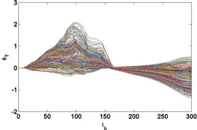
The DPC plot of figure 2 is an example for an in-silico single spiral wave in a fixed instant of time chosen here randomly around 𝑡𝑡𝑘𝑘=100 ms. This choice is based on the behavior of the body-surface potentials of figure 1 and in the literature [23].
Fig. 1. In-silico body-surface potentials, Φ𝑇𝑇 for 𝑡𝑡𝑘𝑘= 1, ⋯ , 300ms (corresponding to the first beat) of the single spiral wave used for the DPC plot example of figure 2.
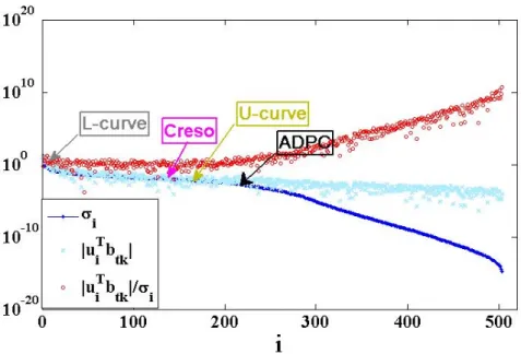
Fig. 2. DPC plot for a time , 𝑡𝑡𝑘𝑘 (𝑚𝑚𝑚𝑚) using the regularization toolbox of Matlab [22] from PC.
Hansen The dot points show the decay of 𝜎𝜎𝑖𝑖, the crosses �𝑢𝑢𝑖𝑖𝑇𝑇𝑏𝑏𝑡𝑡𝑘𝑘�, and the circles the quotient between both. The values of the different regularization parameter choices are located in the plot with different color arrows and their respective methods’ name.
The DPC plot above shows the ill-posedness of the inverse problem. We can see that after the index 𝑖𝑖~240 SVs (being 𝑁𝑁𝑇𝑇=252), the data become dominated by errors/noise and the solution (3) starts to become instable and affected by them. This is due to the fact that for 𝑖𝑖 >240, the SVs (dot points), 𝜎𝜎𝑖𝑖, start to decrease to zero faster than the right hand side coefficients (crosses) and the DPC fails for any regularization parameter below 𝜎𝜎240. Besides, by holding different color arrows for the different parameter choices on the DPC plot, we can observe the over-regularization provided by the L-curve method.
We want to remark that while here we only plot the DPC for a certain spiral wave data and for a fixed instant of time, 𝑡𝑡𝑘𝑘, (as example to explain the details of a DPC plot) the SVs for the ECGI MFS matrix as formulated in [9,10] usually decrease slowly initially, and they start to highly decrease for larger values of the index 𝑖𝑖 (commonly 𝑖𝑖~𝑁𝑁𝑇𝑇). The same SV decay behavior for ECGI MFS for other real torso-heart geometries can be observed in [24].
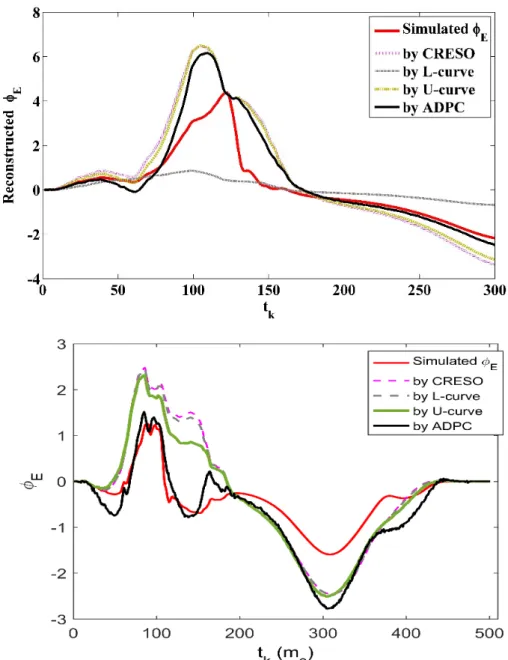
Figure 3 shows the reconstructed potentials in a random location on the epicardium through the different time instants, 𝑡𝑡𝑘𝑘 (ms) for the different regularization parameters together with the simulated ones. We observe that in this example the solution based on the L-curve is over-regularized.
Fig. 3. Signal reconstructed in a point of the epicardium along the time for the different
regular-ization parameters methods as legend indicates against the simulated one. Above: Single site pacing data in the RV, below: single site pacing data in the LV.
3.2 Correlation coefficients and relative errors of reconstructed potentials in time and activation time maps
Table 1 presents the three quartiles of CCs, RMSEs and REs of the reconstructed potentials with the different regularization parameters found for the single site pacing simulations (SSPs) and single spiral waves simulations (SSWs). Table 2 shows the min-imum, median, and maximum of CCs and REs of the respective activation time (AT) maps. In both tables the best CCs, RMSEs and/or REs are outlined in red color.
Method Dataset CCs RMSEs REs (L2-norm)
CRESO SSPs 0.77 [0.49, 0.86] 0.05 [0.04, 0.06] 0.81 [0.62, 1.03] SSWs 0.74 [0.57, 0.86] 0.07 [0.05, 0.10] 0.77 [0.64, 0.96] L-curve SSPs 0.76 [0.51, 0.85] 0.05 [0.04, 0.06] 0.89 [0.67, 1.06] SSWs 0.70 [0.46, 0.82] 0.08 [0.05, 0.13] 0.91 [0.80, 1.08] U-curve SSPs 0.76 [0.53, 0.86] 0.06 [0.05, 0.08] 0.80 [0.60, 0.97] SSWs 0.76 [0.60, 0.87] 0.07 [0.05, 0.09] 0.75 [0.61, 0.93] ADPC SSPs 0.81 [0.70, 0.89] 0.06 [0.04, 0.08] 0.71 [0.54, 0.83] SSWs 0.81 [0.68, 0.90] 0.06 [0.04, 0.09] 0.69 [0.55, 0.87]
Table 1. Median [1st quartile, 3rd quartile] of the: CCs, RMSE and REs of the reconstructed
potentials along the time.
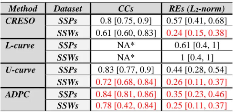
Method Dataset CCs REs (L2-norm)
CRESO SSPs 0.8 [0.75, 0.9] 0.57 [0.41, 0.68] SSWs 0.61 [0.60, 0.83] 0.24 [0.15, 0.38] L-curve SSPs NA* 0.61 [0.4, 1] SSWs NA* 1 [0.4, 1] U-curve SSPs 0.83 [0.77, 0.9] 0.44 [0.28, 0.54] SSWs 0.72 [0.68, 0.84] 0.26 [0.11, 0.37] ADPC SSPs 0.84 [0.81, 0.86] 0.35 [0.23, 0.46] SSWs 0.78 [0.42, 0.84] 0.25 [0.11, 0.37]
Table 2. Median [min, max] of the CCs and of the REs for the activation time (AT) maps.
NA*: Not applicable because the computation of the ATs is inhibited due to the over-regularized solution provided by L-curve.
4
Discussion and Conclusions
We presented ADPC, a new method to choose the regularization parameter for Tikhonov regularization and we showed the feasibility of this new method and the ex-istent U-curve method (never before used for ECGI problems). Our results showed the importance of the choice of the regularization parameter.
For the in-silico data used here, we found that the L-curve provided an over-regular-ized solution for the single site pacing (SSP) in the RV and for three of the single spiral waves simulations (SSWs), inhibiting the computation of the AT map for these SSWs. In figure 2, for one of the SSWs, we can clearly see how the L-curve regularization parameter provided is far above the other regularization parameters, as well as of the moment where the SVs start to decay to zero faster than the respective right hand side coefficients. For the cases that this happens, a few SVs are highly weighted in the Tikhonov solution (3), and this results in a highly over-regularized solution. In figure 3 (above), we can visualize this fact in terms of the reconstructed potentials in a random epicardial point along the time (for a SSP in the RV); when using the L-curve regular-ization parameter. Furthermore, figure 3 (below) shows that ADPC improves also the reconstruction in a SSP in the LV.
While CRESO seems to give lower RMSE in agreement with the work of Rudy [10]
for the single site pacing simulations (table 1), the U-curve and specially the ADPC provide higher CCs in terms of potentials (in time) and lower REs. Furthermore, the CCs of the ATs are also higher for the U-curve and the ADPC, especially for the SSWs (5-11% of improvement), while the REs are not affected for the SSWs and decreased for the SSPs in a 21% respect to the usual CRESO method (table 2).
We would like to remark that this study provides results for the ECGI MFS problem, such as described in [9,10]. However, it is well known that a suitable automatic regular-ization parameter choice method depends on the inverse problem treated [12]. There-fore, if the ECGI problem is numerically approximated by a different method such as the finite element method or the boundary element method, this study must be repeated for the specific problem in each case. DPC provides an interval that any Tikhonov reg-ularization parameter should fulfill. The empirical choice of the lower threshold for the ADPC algorithm is working well for the ECGI MFS problem [9,10] where the decay behavior of SVs does not have jumps and always decays slowly for the first SVs 𝑖𝑖~𝑁𝑁𝑇𝑇, 𝑖𝑖≤ 𝑁𝑁𝑇𝑇, and the respective coefficients of the solution start to be unstable exactly at that moment. The empirical lower threshold of DPC (step 3), chosen in our ADPC algo-rithm, may be differently adapted for others approaches with different SV decayment behavior. More detail of DPC can be found in earlier work [12,18] that may help to the reader to adapt it to a specific inverse problem. Equally in different inverse problems involving spatio-temporal solutions, the choice of the mode or mean instead of median could be more accurate for step 4 than the median proposed here. Nevertheless, we believe that, as shown for our specific problem, a good adaptation of ADPC for each different numerical approach of ECGI or other ill-posed problems should provide suit-able results since ADPC is really focused on the mathematical DPC that any Tikhonov solution should fulfill.
Finally, it seems advisable to test the four regularization parameter choice methods with experimental data with different pathologies and study the different solutions in future work.
Acknowledgements. This study received financial support from the French
Agency (ANR), Grant reference ANR-10-IAHU-04 and from the Conseil Régional Aq-uitaine as part of the project “Assimilation de données en cancérologie et cardiologie”. This work was granted access to the HPC resources of TGCC under the allocation x2016037379 made by GENCI.
References
1. Shah, A. (2015). Frontiers in Noninvasive Cardiac Mapping, an Issue of Cardiac Electrophys-iology Clinics. Elsevier Health Sciences, 7 (1).
2. Rudy Y. (2013). Noninvasive electrocardiographic imaging of arrhytmogenic substrates in humans. Circulation research, 112, 849-862.
3. Wang, Y., et al. (2011). Noninvasive electro anatomic mapping of human ventricular arrhyth-mias with electrocardiographic imaging. Science translational medicine, 3(98), 98ra84-98ra84.
4. Ramanathan, C., et al. (2004). Noninvasive electrocardiographic imaging for cardiac electro-physiology and arrhythmia. Nature medicine, 10(4), 422-428.
5. Dubois R., et al. (2015). Non-invasive cardiac mapping in clinical practice: Application to the ablation of cardiac arrhythmias. Journal of Electrocardiology, 48(6), 966-974.
6. Haissaguerre M, et al. (2013). Noninvasive panoramic mapping of human atrial fibrillation mechanisms: a feasibility report. Journal of Cardiovascular Electrophysiology, 24, 711-717. 7. Cochet, H., et al. (2014). Cardiac arrythmias: multimodal assessment integrating body surface
ECG mapping into cardiac imaging. Radiology, 271(1), 239-247.
8. Cluitmans, M. J. M., et al. (2015). Noninvasive reconstruction of cardiac electrical activity: update on current methods, applications and challenges. Netherlands Heart Journal, 23(6), 301-311.
9. Wang Y., & Rudy Y. (2006). Application of the method of fundamental solutions to potential-based inverse electrocardiography. Annals of Biomedical Engineering, 34, 1272-88.
10. Rudy, Y. (2004). U.S. Patent No. 6,772,004. Washington, DC: U.S. Patent and Trademark Office.
11. Milanič, M., et al. (2014). Assessment of regularization techniques for electrocardiographic imaging. Journal of electrocardiology, 47(1), 20-28.
12. Hansen, P. C. (2010). Discrete inverse problems: insight and algorithms (Vol. 7). SIAM. 13. Tsai, C. C., et al. (2006). Investigations on the accuracy and condition number for the method
of fundamental solutions. Computer Modeling in Engineering and Sciences, 16(2), 103. 14. Colli-Franzone, P., et al. (1985). A mathematical procedure for solving the inverse potential
problem of electrocardiography. Analysis of the time-space accuracy from in vitro experi-mental data. Mathematical Biosciences, 77(1-2), 353-396.
15. Ruan, S., Wolkowicz, G. S. K., & Wu, J. (Eds.). (1999). Differential equations with
applica-tions to biology (Vol. 21). American Mathematical Soc.
16. Hansen, P. C., & O’Leary, D. P. (1993). The use of the L-curve in the regularization of discrete ill-posed problems. SIAM Journal on Scientific Computing, 14(6), 1487-1503.
17. Krawczyk-Stańdo, D., & Rudnicki, M. (2007). Regularization parameter selection in discrete ill-posed problems—the use of the U-curve. International Journal of Applied Mathematics
and Computer Science, 17(2), 157-164.
18. Chamorro-Servent, J., et al. (2011). Feasibility of U-curve method to select the regularization parameter for fluorescence diffuse optical tomography in phantom and small animal studies.
19. Duchateau, J., Potse, M., & Dubois, R. (2016). Spatially Coherent Activation Maps for Elec-trocardiographic Imaging. IEEE Transactions on Biomedical Engineering, (in print). 20. Ten Tusscher, K. H. W. J., et al. (2004). A model for human ventricular tissue. American
Journal of Physiology-Heart and Circulatory Physiology, 286(4), H1573-H1589.
21. Potse, M. et al. (2009). Cardiac anisotropy in boundary-element models for the electrocardi-ogram. Medical and Biological Engineering and Computing, 47(7), 719-729.
22. Hansen, P. C., Regularization Tools Version 4.0 for Matlab 7.3, Numerical Algorithms, 46 (2007), pp. 189-194.
23. Ghodrati, A., et al. (2006). Wavefront-based models for inverse electrocardiography. IEEE
transactions on biomedical engineering, 53(9), 1821-1831.
24. Chamorro-Servent, J., et al. (2016, September). Adaptive placement of the pseudo-boundaries improves the conditioning of the inverse problem. In Computing in Cardiology, 43, 705-708.