Combining a Renewable Portfolio Standard with a
Cap-and-Trade Policy: A General Equilibrium Analysis
by MASSACHU!
OF TE(
Jennifer F. Morris
JUN
B.A., Public Policy Analysis and History
LIBF
University of North Carolina at Chapel Hill, 2006 Submitted to the Engineering Systems Division in Partial Fulfillment of the Requirements for the Degree of
Master of Science in Technology and Policy at the
Massachusetts Institute of Technology June 2009
@2009 Massachusetts Institute of Technology. All rights reserved.
Signature of Author...
Certified by... . ...
Accepted by ...
Professor(of
ARCHIVES
Engineering Systems Division May 8, 2008
Dr. John M. Reilly enior Lecturer, Sloan School of Management Thesis Supervisor
...
Dr. Dava J. Newman Aeronautics and Astronautics and Engineering Systems Director, Technology and Policy Program
Combining a Renewable Portfolio Standard with a
Cap-and-Trade Policy: A General Equilibrium Analysis
by
Jennifer F. Morris
Submitted to the Engineering Systems Division on May 8, 2009 in Partial Fulfillment of the Requirements for the Degree of Master of Science in
Technology and Policy
ABSTRACT
Most economists see incentive-based measures such a cap-and-trade system or a carbon tax as cost effective policy instruments for limiting greenhouse gas emissions. In actuality, many efforts to address GHG emissions combine a cap-and-trade system with other regulatory instruments. This raises an important question: What is the effect of combining a cap-and-trade policy with policies targeting specific technologies?
To investigate this question I focus on how a renewable portfolio standard (RPS) interacts with a cap-and-trade policy. An RPS specifies a certain percentage of electricity that must come from renewable sources such as wind, solar, and biomass. I use a computable general equilibrium (CGE) model, the MIT Emissions Prediction and Policy Analysis (EPPA) model, which is able to capture the economy-wide impacts of this combination of policies. I have represented
renewables in this model in two ways. At lower penetration levels renewables are an imperfect substitute for other electricity generation technologies because of the variability of resources like wind and solar. At higher levels of penetration renewables are a higher-cost prefect substitute for other generation technologies, assuming that with the extra cost the variability of the resource can be managed through backup capacity, storage, long range transmissions and strong grid connections. To represent an RPS policy, the production of every kilowatt hour of electricity from non-renewable sources requires an input of a fraction of a kilowatt hour of electricity from renewable sources. The fraction is equal to the RPS target.
I find that adding an RPS requiring 25 percent renewables by 2025 to a cap that reduces emissions by 80% below 1990 levels by 2050 increases the welfare cost of meeting such a cap by 27 percent over the life of the policy, while reducing the CO2-equivalent price by about 8 percent each year.
Thesis Supervisor: Dr. John M. Reilly
ACKNOWLEDGEMENTS
The Joint Program on the Science and Policy of Global Change at MIT has been a truly amazing place to work. I cannot imagine a better group of people to work with and learn from every day. I cannot thank John Reilly, my research supervisor, enough for his priceless guidance and insight throughout my time here. I am also unbelievably grateful for the invaluable help and support given to me by Sergey Paltsev. I could not have finished my thesis without him. John and Sergey have taught me so much, and have also been wonderful sources of comic relief and good laughs. I also extend heartfelt appreciation to Jake Jacoby and Mort Webster for their interest in my work, suggestions, and meaningful support. I also need to thank Fannie Barnes and Tony Tran for the fantastic assistance and company they provide to us all at the Joint Program. I further thank the Joint Program sponsors, including the U.S. Department of Energy, U.S.
Environmental Protection Agency and a consortium of industry and foundation sponsors, who have supported the development of the EPPA model used in this work.
In addition, I am grateful to the Technology and Policy Program (TPP) which has provided me with a wonderful academic experience. I particularly thank Sydney Miller for all she does for TPP and all the help she has given me during my time here. I extend further thanks to my fellow JP and TPP students who have made my time here so enjoyable.
Finally, I would like to thank my family and friends for their support and all of the fun times which gave me a break from work and school. I particularly thank my husband Josh for his amazing love, support and encouragement, and his patience in listening to me talk about the EPPA model. I thank my mom, dad, brothers, in-laws, and extended family for their enduring love and support. I dedicate this thesis to my grandfather who was always so proud of me and the work I was doing. It is my hope that this work can be used to inform climate policy discussions.
TABLE OF CONTENTS
1. INTRODUCTION...8
2. RENEWABLE PORTFOLIO STANDARDS AND CLIMATE POLICY...10
2.1 Renewable Portfolio Standards ... .. ... 10
2.2 Focus on RPS in Climate Legislation ... 13
2.3 U.S. State-Level RPS Policies ... 17
3. ISSUES AFFECTING THE COSTS OF RENEWABLES ... .. 20
3.1 E xisting Public Policies ... ... .... ... ... 20
3.2 Intermittency and the Need for Storage or Backup ... 21
3.3 Transmission and Grid Connections ... 22
4. ANALYSIS METHOD ... 24
4.1 A Computable General Equilibrium (CGE) Model for Energy and Climate Policy... 24
4.2 The Emissions Prediction and Policy Analysis (EPPA) Model ... 24
4.3 Representing Renewables and Renewable Policy... 27
4.3.1 Renewable Technologies... 28
4.3.2 RPS Constraint ... ... 35
5. ECONOMICS OF RENEWABLE PORTFOLIO STANDARDS ... 36
5.1 Effects of the Revised Model... ... ... 38
5.2 Im pact of RPS Policy ... 45 5.2.1 RPS Only... 46 5.2.2 RPS with Cap-and-Trade ... 49 5.3 Sensitivity ... ... 59 6. CONCLUSIONS ... 66 7. REFERENCES... 68
LIST OF TABLES
Table la. Congressional Cap-and-Trade Bills, Basic Features... ... 14
Table lb. Congressional Cap-and-Trade Bills, Additional Details and Features. ... 15
Table ic. Congressional Cap-and-Trade Bills, Additional Details and Features (continued)... 16
Table 2. State Renewable Portfolio Standards ... 18
T able 3. 2002 Costs of Texas RPS... 23
T able 4. EPPA M odel D etails ... .. ... 26
Table 5. Cost Calculation of Electricity from Various Sources... 31
Table 6. Cost Shares for Electricity Generating Technologies: (a) Existing Technologies and (b) N ew Technologies. ... 33
Table 7. RPS Targets and Timetables (a) in Congressional Bills, and (b) Used in EPPA... 45
Table 8. Net Present Value Welfare Change 2015-2050. ... ... 48
Table 9. Welfare Change and C02-e Price of Congressional Proposals ... 56
LIST OF FIGURES
Figure 1. New Additions of Non-hydroelectric Renewable Capacity in the U.S. 1991-2007... 19
Figure 2. Production Function for Electricity from Wind with Biomass Backup. ... 34
Figure 3. Production Function for Electricity from Wind with NGCC Backup ... 34
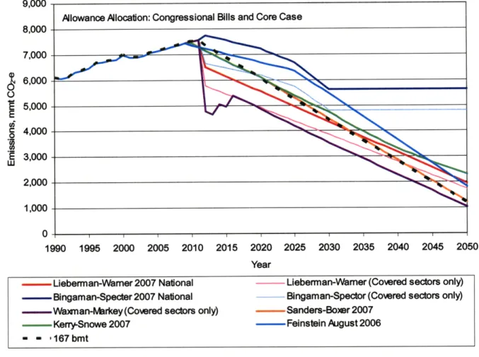
Figure 4. Scenarios of allowance allocation over time ... ... 37
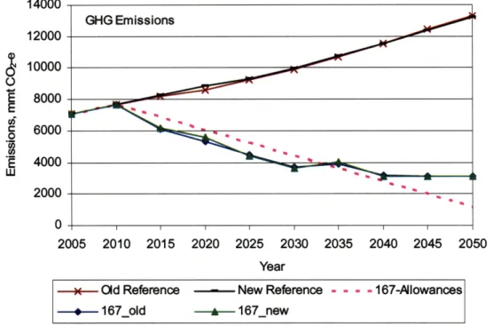
Figure 5. GHG Emissions in Old and New Model. ... .. ... 39
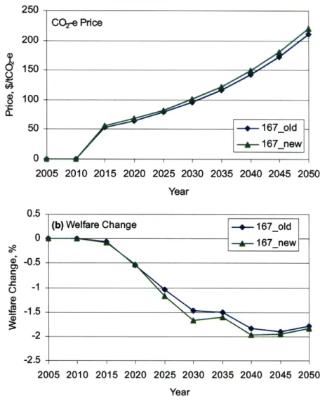
Figure 6. (a) CO2-e Prices and (b) Welfare Changes in Old and New Model... 40
Figure 7. Electricity Generation by Source (a) Reference Case, (b) 167 bmt in Old Model, and (c) 167 bm t in N ew M odel. ... 42
Figure 8. Electricity Generation by Source (a) 167 bmt with No CCS, (b) 167 bmt with No CCS and High Gas Cost, (c) 167 bmt with No CCS and Low Wind with Backup Cost... 44
Figure 9. GHG Em issions Paths. ... 49
Figure 10. W elfare Change. ... 47
Figure 11. Electricity Generation by Source (a) Reference and (b) RPS Only ... 42
Figure 12. GHG Em issions Paths. ... 49
Figure 13. 2030 Welfare Change at Various Levels of RPS Targets. ... 50
Figure 14. 2030 CO2-e Price at Various Levels of RPS Targets ... 51
Figure 15. MAC Curves with and without an RPS... 53
Figure 16. GHG Em issions Paths. ... 54
Figure 17. W elfare Change. ... 55
Figure 18. CO 2-e Price. ... 56
Figure 19. Electricity Generation by Source: (a) 167 bmt, (b) 167 bmt with RPS, and (c) RPS O nly... ... 57
Figure 20. Electricity Price Index. ... 59
Figure 21. Welfare Change: (a) 167 bmt, (b) 167 bmt with RPS, and (c) RPS Only. ... 60
Figure 22. CO2-e Prices. ... 62
Figure 23. Electricity Generation by Source for the 167bmt with RPS Policy in: (a) the Base Case, (b) the high CCS cost case, and (c) the high renewables cost case. ... 63
1. INTRODUCTION
There are two main categories of policy instruments to reduce emissions: economic incentive approaches and command-and-control approaches. From the first category is a cap-and-trade policy, which places a limit on the total quantity emissions. All covered entities must submit a permit or allowance for every ton of emissions produced, and the total number of allowances in existence equals the national cap. Covered entities can trade allowances, which creates a market for allowances and establishes a price on emissions, which in turn creates economic incentives for abatement.' Command-and-control measures are conventional regulations, for example mandating that specific technologies be used.
Most economists see incentive-based measures such as a cap-and-trade system or an emissions tax as cost effective instruments for limiting greenhouse gas (GHG) emissions. In actuality, many efforts to address GHG emissions combine a cap-and-trade system with
regulatory instruments. This raises an important question: What is the effect of combining a cap-and-trade policy with policies targeting specific technologies?
To investigate this question I focus on how a renewable portfolio standard (RPS) interacts with a cap-and-trade policy. An RPS specifies a certain percentage of electricity that must come from renewable sources such as wind, solar, and biomass. RPS policies have gained increasing focus in climate policy, and have already been implemented in some places. The European Union's 20-20-20 goal includes achieving a 20% renewables energy mix by 2020, which is commonly implemented through an RPS. Many states in the U.S. have implemented state-level RPS policies. Further, the majority of U.S. cap-and-trade bills include a national RPS. With so much attention on RPS, it is important to study how such a policy interacts with a cap-and-trade policy.
To do this, I use a computable general equilibrium (CGE) model. Because I am looking at policies that impact sectors throughout the economy, it is crucial to capture all of the interaction and ripple effects. A CGE model is able to do this and is therefore a particularly appropriate tool to assess the economy-wide impacts of these policies. I use the MIT Emissions Prediction and Policy Analysis (EPPA) model, which is developed specifically to evaluate the impact of energy and environmental policies on the global economic and energy systems.
For a discussion of the history of cap-and-trade systems in the US and analysis of their application to CO2 see
I have represented renewable technologies in the EPPA model in two ways. At lower penetration levels renewables are an imperfect substitute for other electricity generation technologies because of the variability of resources like wind and solar. At higher levels of penetration renewables are a higher-cost perfect substitute for other generation technologies, assuming that with the extra cost the variability of the resource can be managed through backup capacity, storage, long range transmissions and strong grid connections. To represent an RPS policy, the production of every kilowatt hour of electricity from non-renewable sources requires an input of a fraction of a kilowatt hour of electricity from renewable sources. The fraction is equal to the RPS target.
The Chapters are organized as follows: Chapter 2 looks at the recent focus on RPS policies in other countries, states within the U.S. and proposed national legislation in the U.S. Chapter 3 reviews the issues affecting the costs of renewable generation, such as government support, intermittency, storage and backup, and long distance transmission and grid connections, which must be accounted for in a CGE model. In Chapter 4 I1 describe the CGE model I use, and how I modified it to better represent renewable technologies and to implement an RPS constraint. Chapter 5 explores the effect of the adding the new technologies to the model and then uses the new RPS constraint to assess the impacts of an RPS policy, both alone and combined with a cap-and-trade policy. Those results are also compared to a cap-cap-and-trade only policy. I also explore the sensitivity of the results to different assumptions about the costs of generating technologies. In Chapter 6 I offer some conclusions.
2. RENEWABLE PORTFOLIO STANDARDS AND CLIMATE POLICY 2.1 Renewable Portfolio Standards
A renewable portfolio standard (RPS) is a policy that requires that a minimum amount of electricity come from renewable energy sources, such as wind, solar, and biomass. The standard could be expressed in a number of ways, such as the number of megawatts of installed capacity, the percentage of installed capacity, the percentage of electricity produced, or the percentage of electricity sold at retail. Most commonly the RPS is in terms of percentage of electricity sold at retail; for example by 2020 20% of electricity sold must come from renewables. The energy sources qualifying as "renewable" to meet the standard can also vary. Wind, solar (solar thermal and photovoltaic), biomass, and geothermal are generally always eligible. Hydroelectricity may or may not be eligible. A commonly proposed rule is that existing hydroelectric generation does not count, but incremental new hydroelectricity does (EIA, 2007a). Municipal solid waste and landfill gas are sometimes included. Some argue that the standard should be expanded to low-carbon technologies like nuclear, integrated coal gasification combined cycle (IGCC) plants and plants with carbon capture and sequestration (CCS), but almost none of the existing RPS policies or proposals consider these technologies eligible.
Many RPS programs utilize tradable renewable electricity certificates (RECs) to increase the flexibility and reduce the cost of meeting the target. A REC is created when a specified amount (e.g. kilowatt-hour or megawatt-hour) of renewable electricity is generated, and it can be traded separately from the underlying electricity generation. REC transactions create a second source of revenue for renewable generators, which functions like a subsidy. RECs also offer flexibility to retail suppliers by allowing them to comply by either directly purchasing renewable electricity or by purchasing RECs. Banking and borrowing of RECs may also be allowed for flexibility.
Another design option is "tiered" targets. Tiered targets establish different sets of targets and timetables for different renewable technologies (for example, one target for solar and another for wind and biomass). The purpose of tiers is to ensure that an RPS provides support to not just the least-cost renewable energy options, but also to certain "preferred" resources such as solar power (DeCarolis and Keith, 2006). However, this design option is not common as it makes compliance with the target more expensive by mandating technologies other than the least-cost renewables.
An RPS is often advanced as part of a package to address climate change. An important economic concept is that policy should correct market externalities. An array of economic work
supports broad incentive-based measures, such as a cap-and-trade system, over technology specific measures for addressing environmental externalities such as climate change (for
example, Baumol and Oates, 1988; Tietenberg, 1990; Stavins, 1997; Palmer and Burtraw, 2005; Dobesova et al., 2005). Fischer and Newell (2004) compared the partial equilibrium social cost of different policies using a simple economic model of electricity markets. They found that an RPS set to achieve a 5.8% reduction in carbon emissions is 7.5 times as costly in terms of social welfare as using an emissions tax (assumed equivalent to a cap-and-trade) to achieve the same emissions reductions. By shifting investment away from the least-cost emission reduction options and toward specific renewable technologies, which are not necessarily least-cost or even low-cost, an RPS adds to the economy-wide cost of the policy. Theoretical analysis also
generally concludes that economic instruments are more efficient than regulatory mechanisms at promoting technical change (Jaffe et al., 1999; Jaffe and Stavins, 1995). Regulations provide no incentive for firms to make improvements beyond the standards imposed whereas taxes and permits provide continual incentive to reduce pollution control costs. Also, a technology standard like an RPS can result in technological lock-in of solutions that are not the best.
Unlike an RPS, a carbon pricing policy (a cap-and-trade or emissions tax) does not attempt to pick winning technologies. By forcing fossil fuels to internalize the cost of their emissions, a cap-and-trade system indiscriminately provides an advantage to technologies in proportion to the level of emissions they produce, and lets the market choose the least-cost options that achieve to the emissions goal. The market may choose renewables, but it may not- it may instead choose nuclear or CCS. But the winning technologies themselves are not the point, the point is that the emissions target is being met, and is being met in the least-cost way.
Another common argument in support of an RPS is that it is necessary for the development of renewable technologies. There are cases made for intervention in the market when technologies are underdeveloped. Development of new technologies requires gradual learning by doing or learning by using (Arrow, 1962; Dosi, 1988; Mann and Richels, 2004). Thus, it is not because a particular technology is efficient that it is adopted, but rather because it is adopted that it will become efficient (Arthur, 1989). An RPS policy, which forces adoption of renewable
technologies, may be appropriate if there are market barriers preventing their adoption, and hence development. Such barriers may exist due to the public good nature of knowledge or learning and scale effects that may act as market barriers for new technologies. Knowledge
gained from research, development and deployment can be shared by people outside of the investment and can spillover to other technologies. These positive externalities are not factored into investment decisions and as a result there is an underinvestment in RD&D compared to what is optimal from a social welfare perspective. Also, renewable technologies, like any new
technology, have to compete with established technologies which have benefited for a long time from scale, mass production and learning effects, all of which lower costs. When renewables arrive on the market, they have not reached an ideal level of performance in terms of cost and reliability, and hence cannot compete and remain underdeveloped. It can then be argued that an RPS is needed to incentivize investment in and the adoption of renewable technologies.
Otto and Reilly (2007) investigated the need for policies targeting specific low-carbon technologies. They found that when technology externalities exist, adoption or R&D subsidies
added to a CO2 trading scheme can increase the cost-effectiveness of achieving an abatement target by internalizing the externalities. An RPS can be considered an adoption subsidy as it
forces renewables into the market. However, they noted that depending on the target, a CO2 trading scheme alone can be sufficient to induce adoption of low-carbon technologies, alleviating the need for technology specific policies. A cap-and-trade policy at the levels being discussed today (80% below 1990 or 2005 levels) would likely provide sufficient incentive to stimulate dynamic learning for whatever technology the market chooses.
Even if barriers do exist, they would vary by technology in such a way that a generic RPS would not address all of them. Renewable technologies have reached different stages of maturity, and the type of support given to each should therefore be adapted. This might range from R&D support for emerging technologies to information and communication support for those
technologies that have already demonstrated their profitability (Christiansen, 2001). The privileged market access afforded by an RPS is likely to be of greatest value in accelerating the progress of early-stage technologies toward competitiveness with conventional fuels in a carbon pricing world, and of least value when extended to mature technologies. Since wind is by far the most mature, it has the least need for RPS support, but because it is the cheapest it would likely dominate, as has been the experience in U.S. states. Further, barriers are not unique to renewable technologies, but are also faced by technologies like CCS and nuclear. It is unclear why
renewables would merit directed support while other technologies would not. In addition, most market barriers are to initial entry and should be overcome once a technology achieves a low
percentage of the generation mix, well below the percentage targets in proposed and existing RPS policies. In the U.S., state RPS policies have likely already served that purpose. Thus for this study I am assuming that these barriers are already solved.
2.2 Focus on RPS in Climate Legislation
RPS policies are being implemented or proposed more and more frequently, making the study of their impacts increasingly important. A number of countries have already implemented
renewable portfolio standards. In 2008 the European Union announced its 20-20-20 goal, which includes achieving a 20% renewables energy mix by 2020.2 Member states are required to adopt national targets consistent with reaching the overall EU target. Several countries have
implemented an RPS with tradable certificates to achieve their national goals, including the United Kingdom, Sweden, Belgium, Italy, and Poland. The European Union is also studying the feasibility, costs, and benefits of implementing a community-wide renewable certificate trading program (ESD 2001, Quen6 2002). Outside of the EU, Australia adopted an RPS for wholesale electricity suppliers beginning in 2001. Japan also has an RPS that includes a price cap on the price of renewable credits (Keiko 2003).
In the United States there have been numerous attempts since 1997 to pass a federal RPS, but none have succeeded. However, a federal RPS is now included in a number of Congressional proposals. There is currently a federal RPS bill in the House by Representative Markey (H.R.890) and one in the Senate by Senator Tom Udall (S.433). The RPS included in the Waxman-Markey draft (The American Clean Energy and Security Act of 2009) has the same time schedule of RPS targets as these bills, which is 25% renewable electricity by 2025. The RPS proposals include REC trading, limited banking and borrowing of RECs (within 3 years), alternative compliance payments, penalties, a renewable electricity deployment fund, and sunset provisions, among other features. In addition to stand-alone federal RPS plans, a number of proposed cap-and-trade bills also include an RPS. A selection of U.S. cap-and-trade proposals is presented in Table la, b, and c. As the "Other Features" row of Table 1c shows, the majority of Congressional cap-and-trade bills incorporate command-and-control, technology-specific
measures, particularly an RPS.
2 The other components of the EU 20-20-20 target are a 20% reduction in CO
2 and a 20% increase in energy efficiency, both by 2020.
Table la. Congressional Cap-and-Trade Bills, Basic Features.
Lieberman-Warner 2007 Bingaman-Specter Kerry-Snowe 2007 Sanders-Boxer 2007 Waxman-Markey Feinstein August
2007 Draft 2009 2006
Bill Number/ S.2191; America's Climate S.1766; Low Carbon S.485; Global Warming S.309; Global Draft; American Clean
Name Security Act of 2007 Economy Act of 2007 Reduction Act of 2007 Warming Pollution Energy and Security
Reduction Act of 2007 Act of 2009
Basic Mandatory, market-based, Mandatory, market- Mandatory, market- Mandatory, market- Mandatory, market- Mandatory,
market-Framework cap on total emissions for based cap on total based, cap on total based, system to be based, cap on total based, cap on total all large emitters: cap & emissions for all large emissions for all large determined by EPA, emissions for all large emissions for all trade emitters: cap & trade emitters: cap & trade allows for cap & trade emitters: cap & trade large emitters: cap
with safety valve (TAP) in 1 or more sectors & trade
Targets Return emissions to 2005 Return emissions to Gradually reduce to Achieve 1990 levels 3% below 2005 levels Cut emissions to levels by 2012, then 2006 levels by 2020, 65% below 2000 levels by 2020, reduce by 1/3 by 2012, 20% below 70% below 1990 gradually reduce to 70% 1990 levels by 2030, by 2050: 1990 levels of 80% below 1990 2005 levels by 2020, levels by 2050. below 2005 levels by and at least 60% below by 2020, then reduce by levels by 2030, by 2/3 42% below 2005 levels
2050. (different targets for 2006 levels by 2050 (set 2.5% per yr between of 80% below 1990 by 2030, and 83%
HFCs) allowances up to 2030, 2020 and 2029, and levels by 2040, and below 2005 levels by
then contingent on 3.5% per yr between 80% below 1990 2050. (different targets
global effort) 2030 and 2050. levels by 2050. for HFCs)
Allocation of Table of yearly percent Table of yearly percent Undetermined percent Undetermined Undetermined Undetermined
Allowances auctioned: starts with auctioned: starts with auctioned, balance allocation, any auctioning and auctioning and
22.5% in 2012, ends with 24% in 2012, increased allocated free allowances not allocation allocation
70.5% 2031-2050, balance to 53% in 2030, and to allocated to covered
allocated free (portions about 80% by 2050, entities should be
earmarked) balance allocated free given to non-covered
(portions earmarked) entities
Additional * Upstream * Upstream - Total GHGs less than * Less then 3.60F (20C) * Upstream & * Keep temperature Details - Covered entities include * Covered entities 450 ppmv temperature increase, Downstream mix increase to I or 20C
80% of national emissions produce over 80% of * Banking and total GHGs less * Covered entities
* Covered entities emit, national emissions * Non-compliance than 450 ppmv eventually include 85%
produce or import * Technology penalties * Suggests declining of national emissions
products that emit over Accelerator Payment emissions cap with * Covered entities emit,
10,000 metric tons of (TAP) (safety valve): technology-indexed produce or import
GHGs per year instead of submitting stop price products that emit over
* Separate quantity of allowances can pay 25,000 metric tons of
emission allowances TAP price: $12/mt C02, GHGs per year
(Emission Allowance escalates annually at * Banking
Account) for each year 5% real * Borrowing (up to 15%
from 2012 to 2050 * Banking from 2-5 years into the
* Banking * President can exempt future, with interest)
* Borrowing (up to 15% entities and extend to * Non-compliance
per yr) uncovered entities penalties
* Non-compliance * Non-compliance
Table lb. Congressional Cap-and-Trade Bills, Additional Details and Features.
Lieberman-Warner 2007 Bingaman-Specter Kerry-Snowe 2007 Sanders-Boxer 2007 Waxman-Markey Feinstein August
2007 Draft 2009 2006
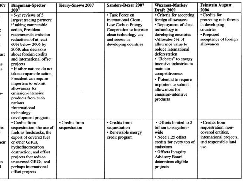
Provisions * Acceptance of foreign * 5-yr reviews of 5 * Task Force on * Criteria for accepting * Credits for
Related to allowances (up to 15%) largest trading partners: International Clean, foreign allowances protecting rain forests Foreign *2.5% of yearly if taking comparable Low Carbon Energy - Deployment of clean in developing Reductions allowances for reducing action, President Cooperation to increase technology to countries
tropical deforestation in recommends emission clean technology use developing countries Proposed
other nations reductions of at least and access in *Allocates 5% of acceptance of foreign
*Help develop and fund 60% below 2006 by developing countries allowance value to allowances
adaptation plans in and 2050, also decisions reduce international
deploy technology to least about foreign credits deforestation
developed nations and international offset * "Rebates" to energy
*Review of other nations: projects intensive industries to
if major emitting nations * If other nations do not maintain
do not take comparable take comparable action, competitiveness
action within 8 yrs, President can require * Potential to require
President can require importers to submit importers to submit
importers to submit allowances for allowances for
allowances for emission- emission-intensive emission-intensive
intensive products from products from such products
such nations nations
-International technology
development program
Credit *Credits from * Credits from * Credits from * Credits from * Offsets limited to 2 * Credits from Provisions sequestration for facilities sequestration, the use of sequestration sequestration billion tons system- sequestration,
non-that do not use coal (for fuels as feedstocks, the * Renewable energy wide covered entities,
coal-using facilities export of covered fuel credit program * Need 1.25 offset international projects,
sequestration reduces their or other GHGs, credits for every ton of and responsible land
allowance submission), hydrofluorocarbon emissions use
emissions that are destruction, and offset * Offsets Integrity
destroyed or used as projects that reduce Advisory Board
feedstocks, offsets (up to uncovered GHGs, and determines eligible
15%) from non-covered perhaps international projects
Table 1c. Congressional Cap-and-Trade Bills, Additional Details and Features (continued).
Lieberman-Warner 2007 Bingaman-Specter Kerry-Snowe 2007 Sanders-Boxer 2007 Waxman-Markey Feinstein August
2007 Draft 2009 2006
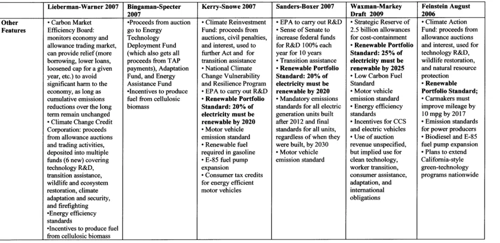
Other * Carbon Market *Proceeds from auction * Climate Reinvestment * EPA to carry out R&D - Strategic Reserve of * Climate Action Features Efficiency Board: go to Energy Fund: proceeds from - Sense of Senate to 2.5 billion allowances Fund: proceeds from
monitors economy and Technology auctions, civil penalties, increase federal funds for cost-containment allowance auctions allowance trading market, Deployment Fund and interest, used to for R&D 100% each * Renewable Portfolio and interest, used for can provide relief (more (which also gets all further Act and for year for 10 years Standard: 25% of technology R&D, borrowing, lower loans, proceeds from TAP transition assistance * Transition assistance electricity must be wildlife restoration, loosened cap for a given payments), Adaptation * National Climate * Renewable Portfolio renewable by 2025 and natural resource
year, etc.) to avoid Fund, and Energy Change Vulnerability Standard: 20% of * Low Carbon Fuel protection
significant harm to the Assistance Fund and Resilience Program electricity must be Standard * Renewable
economy, as long as -Incentives to produce * EPA to carry out R&D renewable by 2020 * Motor vehicle Portfolio Standard; cumulative emissions fuel from cellulosic * Renewable Portfolio * Mandatory emissions emission standard * Carmakers must
reductions over the long biomass Standard: 20% of standards for all electric * Energy efficiency improve mileage by
term remain unchanged electricity must be generation units built standards 10 mpg by 2017
* Climate Change Credit renewable by 2020 after 2012 and final * Incentives for CCS * Emission standards
Corporation: proceeds * Motor vehicle standards for all units, and electric vehicles for power producers
from allowance auctions emission standard regardless of when they * Use of auction - Biodiesel and E-85
and trading activities, * Renewable fuel were built, by 2030 revenue unspecified, fuel pump expansion
deposited into multiple required in gasoline * Motor vehicle but implied use for * Plans to extend
funds (6 new) covering * E-85 fuel pump emission standard clean technology, California-style
technology R&D, expansion worker transition, green-technology
transition assistance, * Consumer tax credits consumer assistance, programs nationwide
wildlife and ecosystem for energy efficient adaptation, and
restoration, climate motor vehicles international
adaptation and security, obligations
and firefighting *Energy efficiency standards
*Incentives to produce fuel from cellulosic biomass
2.3 U.S. State-Level RPS Policies
Within the U.S. many states are not waiting for a federal RPS. In fact, currently 28 states and the District of Colombia have enacted non-voluntary state-level PRS statutes. Five additional states have voluntary RPS programs. Initially, state RPS policies were incorporated into broader state electricity restructuring legislation. More recently, however, state RPS policies have been adopted through stand-alone legislation. Table 2 lists the current state targets. Percentages refer to a portion of electricity sales and megawatts (MW) to absolute capacity requirements. The date refers to when the full requirement takes effect. As of 2007, when 21 states and the District Colombia had an RPS, these policies covered roughly 40% of total U.S. electrical load (Wiser et al., 2007). They have been implemented in both restructured electricity markets and in cost-of-service-regulated markets. Because many of these policies are new, experience remains
somewhat limited, yet immensely varied.
Roughly half of the new renewable capacity additions in the U.S. from the late 1990s through 2006 have occurred in states with RPS policies, totaling nearly 5,500 MW (Wiser et al., 2007). However, state RPS policies are not the only driver of renewable energy development. Other significant motivators include federal and state tax incentives, state renewable energy funds, voluntary green power markets, and the economic competitiveness of renewable energy relative to other generation options. It is immensely challenging to isolate the impacts of the various drivers.
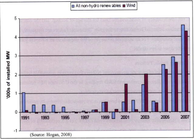
Compliance with the state RPS policies has shown a complete dominance of wind power, with biomass and geothermal playing a small role. Over the past 5 years 97% of all new
renewable generating capacity installed in the U.S. was wind (see Figure 1) (Hogan, 2008). The Independent System Operator and Regional Transmission Organization (ISO/RTO) Council noted in October 2007 that 87% of all the renewable generation in interconnection queues across the country was wind generation (ISO/RTO Council, 2007). EIA (2006) projected that of the capacity stimulated by state RPS programs to 2030, more than 93 percent is estimated to result from large wind farms. Of the eligible renewable resources, terrestrial wind is clearly the most mature and as a result it generally offers the least costly and most immediately accessible option for meeting the RPS targets.
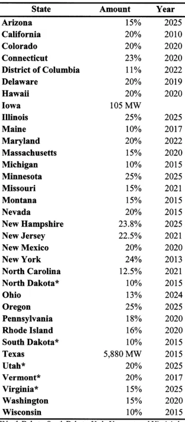
Table 2. State Renewable Portfolio Standards.
State Amount Year
Arizona 15% 2025 California 20% 2010 Colorado 20% 2020 Connecticut 23% 2020 District of Columbia 11% 2022 Delaware 20% 2019 Hawaii 20% 2020 Iowa 105 MW Illinois 25% 2025 Maine 10% 2017 Maryland 20% 2022 Massachusetts 15% 2020 Michigan 10% 2015 Minnesota 25% 2025 Missouri 15% 2021 Montana 15% 2015 Nevada 20% 2015 New Hampshire 23.8% 2025 New Jersey 22.5% 2021 New Mexico 20% 2020 New York 24% 2013 North Carolina 12.5% 2021 North Dakota* 10% 2015 Ohio 13% 2024 Oregon 25% 2025 Pennsylvania 18% 2020 Rhode Island 16% 2020 South Dakota* 10% 2015 Texas 5,880 MW 2015 Utah* 20% 2025 Vermont* 20% 2017 Virginia* 15% 2025 Washington 15% 2020 Wisconsin 10% 2015
*North Dakota, South Dakota, Utah, Vermont, and Virginia have set voluntary goals for adopting renewable energy instead of portfolio standards with binding targets. (Source: North Carolina Solar Center)
m All non-hydro renew ables VWind
4-1
(Source: Hogan, 2008)
Figure 1. New Additions of Non-hydroelectric Renewable Capacity in the U.S. 1991-2007.
3. ISSUES AFFECTING THE COSTS OF RENEWABLES
There are important factors that impact the costs of renewables, including government support, the intermittency of wind and the need for storage or backup, and the construction of new transmission lines and connecting to the grid. These cost factors are frequently left out of price and cost estimates. For an accurate portrayal of the impacts of an RPS it is vital that I capture these costs in my model.
3.1 Existing Public Policies
There are a number of existing government policies that support renewable technologies. These include subsidies, tax credits and R&D funding. In the U.S. state RPS policies also act as subsidies which reduce the perceived cost of renewables.
The production tax credit (PTC) has been the main renewable electricity policy employed at the federal level in the U.S. In 1992, Congress passed the U.S. Energy Policy Act which
authorized a Renewable Energy Production Credit (REPC) of 1.5 cents/kWh of electricity produced from wind and dedicated closed-loop biomass generators. The REPC applied to new generators for the first 10 years of operation. The REPC was extended in 2001, and extended again in 2004 through the end of 2005 and expanded to include geothermal, solar, landfill gas, open-loop biomass, and small hydro. It was extended again and set to expire at the end of 2008. The American Recovery and Reinvestment Act of 2009 (H.R. 1) signed by President Obama extended the PTC until 2012 for wind and until 2013 for other renewables. The PTC acts to reduce corporations' federal tax burden towards levels where only the Alternative Minimum Tax applies. In addition to this production incentive, the Federal government also offers an
investment tax credit (ITC) of 10-30% of capital costs depending on the renewable technology. There are also a number of state-level tax credits and subsidies that support renewables.
It is sometimes assumed that a national RPS policy would simply replace the PTC. However, experience with state RPS policies demonstrates the recurring role of the PTC. In Figure 4 above, the impact of the PTC is notable. The PTC has expired three times during the RPS era without immediately being renewed - the end of 1999, 2001 and 2003. Each time it was belatedly reinstated about a year later. The result each time was a notable drop in the pace of renewables development (see 2000, 2002, and 2004 in Figure 4). So even with the RPS, the PTC has been playing a crucial role in renewable development. Also, policymakers in states that have
implemented RPS programs have relied on the PTC and federal subsidy programs to contain the retail price impact of RPS compliance.
These financial support policies represent a cost to society that is often not included in cost and price estimates of renewable technologies. The expenditures must be paid for by raising other taxes, increasing borrowing, or cutting government programs. So while the incentives reduce producer costs and therefore retail prices, they do so at the expense of the taxpayer, and this welfare cost is typically not considered when calculating the cost of renewables. Also, by keeping electricity prices low, this subsidy leads to more consumption and generation, limiting the effectiveness of reducing carbon.
3.2 Intermittency and the Need for Storage or Backup
The majority of cost and price estimates do not include the costs of intermittency or the costs of capacity reserves or storage needed to maintain system security. These costs particularly apply to wind and solar. Here I focus on wind since it is the dominant renewable. Because of the
intermittency of wind and the temporal mismatch between supply and demand (wind blows more at night when demand for electricity is low), backup capacity and/or storage systems must be put into place. These additional systems have real costs that need to be considered. A study by
DeCarolis and Keith (2006) and found that these costs at all levels of wind penetration amount to 1.1 0/kWh. Strbac (2002) found 0.9 - 1.2 O/kWh for such costs in the U.K.
The intermittency of wind energy affects electricity grids on timescales of seconds to days. System operators are concerned with minute-to-minute, intrahour, and hour to day-ahead scheduling. They employ an automatic generation control (AGC) system to manage minute-to-minute load imbalances. An operating reserve of spinning and nonspinning reserves is capacity that can be dispatched within minutes to respond to forced outages or fluctuations in intrahour load. To meet forecasted demand using economic dispatch, system operators schedule units to produce a specified amount of electricity hours or days in advance. Wind intermittency
complicates economic dispatch, particularly when wind serves a large fraction of demand, because the system operator must balance the risk of wind not meeting its scheduled output against the risk of committing too much slow-start capacity (Milligan, 2000). All else equal, the cost of intermittency will be less if the generation mix is dominated by gas turbines (low capital costs and fast ramp rates) or hydro (fast ramp rates ) than if the mix is dominated by nuclear or coal (high capital costs and slow ramp rates) (DeCarolis and Keith, 2006).
Intermittency can be mitigated by constructing storage facilities or backup capacity integrated with large wind farms, or by adding load following capacity to the wider grid. Storage and backup add to the cost of the wind project and increase the price of electricity. This will be explored more in Chapter 4. Intermittency can also be mitigated by geographically dispersing wind turbine arrays. Geographic dispersion over sufficiently large areas can increase the
reliability of wind by averaging wind power over the scale of prevailing weather patterns. Kahn (1979) quantified the reliability benefit of geographically dispersed wind turbine arrays using California data. More recently, Archer and Jacobson (2003) demonstrated the diversity benefit by comparing the average wind power output across 1 wind site in Kansas, 3 sites across Kansas, and 8 site spanning Kansas, New Mexico, Texas, and Oklahoma. However, such dispersal requires the construction on long-distance transmission lines which are very expensive and also increase the cost of renewables. Intermittency and backup or storage to mitigate it are important costs that need to be accounted for in my model.
3.3 Transmission and Grid Connections
There is also mismatch in the spatial distribution of wind resources and demand. Remote, high-quality, large-scale wind resources are in the middle of the country while electricity demand is on the coasts. This means there is a need for long distance electricity transmission, the costs of which need to be considered.
Existing wind installations are generally located at strong wind sites close to preexisting transmission infrastructure. However, such sites close to demand are not exploitable for
large-scale wind. First, these resources tend to be of lower quality, which makes it more economical to import electricity from distant high quality wind sites (Decarolis and Keith, 2006). Second, the high quality wind sites that do exist near demand centers are generally in environmentally sensitive areas and/or areas where there will be significant public opposition. In the U.S., the controversy surrounding the Cape Wind project is an example of the uproar created by proposals aimed at building wind farms in an area that is both a popular recreational center and
environmentally sensitive (Grant, 2002; Ziner, 2002).
For wind to serve a significant fraction U.S. electricity demand (20% or more), it will need to be located where there is cheap land, low population densities, and strong wind resources. This means the majority of wind capacity will be placed in the Great Plains and transmitted long distances to demand center. A study by Grubb and Meyer, demonstrated that under moderate
land use constraints on wind farm siting, 12 Midwestern states could supply four times the current U.S. demand (Grubb and Meyer, 1993). However, connecting several hundred miles between the Great Plains wind and demand centers would be very costly, and would increase the
price of electricity.
The Dobesova et al. (2005) Texas study attempted to quantify all of the additional costs of the RPS policy. Table 3 shows their accounting of the various costs in 2002, with the total
amounting to close to $76 million. When divided by the total RPS generation, this amounts to 2.7 cents/kWh. If only new renewables are counted, this cost rises to 3.1 cents/kWh. These numbers are added on to the cost of generation. This study, of course, was specific to Texas and cannot simply be extrapolated to the country as a whole. However, it is a useful demonstration of how renewable electricity cost and price estimates often leave out important cost components, thereby underestimating costs. In order for my model to accurately capture the costs of an RPS, it is essential that I account for the additional costs of existing policies, intermittency, and
transmission.
Table 3. 2002 Costs of Texas RPS.
Summary of 2002 Texas RPS costs
Production Tax Credit $44,100,000 Curtailments $18,000,000 Transmission $13,000,000 RPS Administration $663,000
4. ANALYSIS METHOD
4.1 A Computable General Equilibrium (CGE) Model for Energy and Climate Policy Computable General Equilibrium (CGE) models represent the circular flow of goods and services in the economy. They represent the supply of factor inputs (labor and capital services) to the producing sectors of the economy and provide a consistent analysis of the supply of goods
and services from these producing sectors to final consumers (households), who in turn control the supply of capital and labor services (Paltsev et al., 2005). Corresponding to this flow of
goods and services is a reverse flow of payments. Households receive payments from the producing sectors of the economy for the labor and capital services they provide. They then use the income they receive to pay producing sectors for the goods and services consumed. CGE models tracks all of these transactions within and across sectors as well as among countries.
In this way CGE models are very powerful tools for assessing the economy-wide impacts of policies. It is a particularly appropriate tool to study the impacts of emissions reductions and electricity policies. Because these policies impact key sectors of the economy, they affect other sectors throughout the economy. If electricity prices increase, the prices of goods produced by electricity increase, or people have less money to buy other goods. Or electricity may become important to the transportation sector through plug-in electric vehicles. Or biomass may become an important source of electricity generation, thereby affecting the agriculture sector. The point is that policies, especially ones affecting key economic sectors, have ripple effects throughout the entire economy. A CGE model captures all of these ripple and feedback effects. A partial equilibrium model looking just at the electricity sector would not capture all of these interactions and therefore would not get as accurate an estimate of the true economy-wide cost of a policy.
4.2 The Emissions Prediction and Policy Analysis (EPPA) Model
The CGE model that I use is the latest version of the Emissions Prediction and Policy Analysis (EPPA) model developed by the MIT Joint Program on the Science and Policy of Globale Change. The EPPA model is a multi-region, multi-sector recursive-dynamic
representation of the global economy (Paltsev et al., 2005). In a recursive-dynamic solution economic actors are modeled as having "myopic" expectations.3 This assumption means that
3 The EPPA model can also be solved as a forward looking model (Gurgel et al., 2007). Solved in that manner the behavior is very similar in terms of abatement and CO2-e prices compared to a recursive solution with the same model features. However, the solution requires elimination of some of the technological alternatives.
current period investment, savings, and consumption decisions are made on the basis of current period prices.
The EPPA model is built on the GTAP dataset (Hertel, 1997; Dimaranan and McDougall, 2002), which accommodates a consistent representation of energy markets in physical units as well as detailed data on regional production, consumption, and bilateral trade flows. Besides the GTAP dataset, EPPA uses additional data for greenhouse gases and air pollutant emissions based on United States Environmental Protection Agency inventory data.
The model is calibrated based upon data organized into social accounting matrices (SAM) that include quantities demanded and trade flows in a base year denominated in both physical and value terms. A SAM quantifies the inputs and outputs of each sector, which allow for the
calculation of input shares, or the fraction of total sector expenditures represented by each input. Much of the sector detail in the EPPA model is focused on providing a more accurate
representation of energy production and use as it may change over time or under policies that would limit greenhouse gas emissions. The base year of the EPPA model is 1997. From 2000 the model solves recursively at five-year intervals. Sectors are modeled using nested constant
elasticity of substitution (CES) production functions (with Cobb-Douglass or Leontief forms). The model is solved in the Mathematical Programming System for General Equilibrium
(MPSGE) language as a mixed complementarity problem (Mathiesen, 1985; Rutherford, 1995). The resulting equilibrium in each period must satisfy three inequalities: the zero profit, market clearance, and income balance conditions (for more information, see Paltsev et al., 2005).
The level of aggregation of the model is presented in Table 4. The model includes
representation of abatement of CO2 and non-CO2 greenhouse gas emissions (CH4, N20, HFCs,
PFCs and SF6) and the calculations consider both the emissions mitigation that occurs as a byproduct of actions directed at CO2 and reductions resulting from gas-specific control measures. Targeted control measures include reductions in the emissions of: CO2 from the combustion of fossil fuels; the industrial gases that replace CFCs controlled by the Montreal Protocol and produced at aluminum smelters; CH4 from fossil energy production and use,
agriculture, and waste, and N20 from fossil fuel combustion, chemical production and improved fertilizer use. More detail on how abatement costs are represented for these substances is
Non-energy activities are aggregated to six sectors, as shown in the table. The energy sector, which emits several of the non-CO2 gases as well as CO2, is modeled in more detail. The synthetic coal gas industry produces a perfect substitute for natural gas. The oil shale industry produces a perfect substitute for refined oil. All electricity generation technologies produce perfectly substitutable electricity except for Solar and Wind and Biomass which is modeled as producing an imperfect substitute, reflecting intermittent output.
The regional and sectoral disaggregation is also shown in Table 4. There are 16 geographical regions represented explicitly in the model including major countries (the US, Japan, Canada,
China, India, and Indonesia) and 10 regions that are an aggregations of countries. Each region includes detail on economic sectors (agriculture, services, industrial and household
transportation, energy intensive industry) and a more elaborated representation of energy sector technologies. The electricity technologies in red are new additions to the model from this work. Table 4. EPPA Model Details.
Country or Region' Sectors Factors
Developed Final Demand Sectors Capital
United States (USA) Agriculture Labor
Canada (CAN) Services Crude Oil Resources
Japan (JPN) Energy-Intensive Products Natural Gas Resources European Union+ (EUR) Other Industries Products Coal Resources Australia & New Zealand (ANZ) Transportation Shale Oil Resources
Former Soviet Union (FSU) Household Transportation Nuclear Resources Eastern Europe (EET) Other Household Demand Hydro Resources
Developing Energy Supply & Conversion Wind/Solar Resources
India (IND) Electric Generation Land
China (CHN) Conventional Fossil
Indonesia (IDZ) Hydro
Higher Income East Asia (ASI) Nuclear Mexico (MEX) Wind, Solar Central & South America (LAM) Biomass
Middle East (MES) Advanced Gas (NGCC) Africa (AFR) Advanced Gas with CCS Rest of World (ROW) Advanced Coal with CCS
Wind with NGCC Backup Wind with Biomass Backup Fuels
Coal
Crude Oil, Shale Oil, Refined Oil Natural Gas, Gas from Coal Liquids from Biomass Synthetic Gas
When emissions constraints on certain countries, gases, or sectors are imposed in a CGE model such as EPPA, the model calculates a shadow value of the constraint which can be interpreted as a price that would be obtained under an allowance market that developed under a cap and trade system. Those prices are the marginal costs used in the construction of marginal abatement cost (MAC) curves. They are plotted against a corresponding amount of abatement, which is the difference in emissions levels between an unconstrained business-as-usual reference case and a policy-constrained case.
The solution algorithm of the EPPA model finds least-cost reductions for each gas in each sector and if emissions trading is allowed it equilibrates the prices among sectors and gases (using GWP weights). This set of conditions, often referred to as "what" and "where" flexibility, will tend to lead to least-cost abatement. Without these conditions abatement costs will vary among sources and that will affect the estimated welfare cost-abatement will be least-cost within a sector or region or for a specific gas, but will not be equilibrated among them.
The results depend on a number of aspects of model structure and particular input
assumptions that greatly simplify the representation of economic structure and decision-making. For example, the difficulty of achieving any emissions path is influenced by assumptions about population and productivity growth that underlie the no-policy reference case. The simulations
also embody a particular representation of the structure of the economy, including the relative ease of substitution among the inputs to production and the behavior of consumers in the face of changing prices of fuels, electricity and other goods and services. Further critical assumptions must be made about the cost and performance of new technologies and what might limit their market penetration. Alternatives to conventional technologies in the electric sector and in transportation are particularly significant. Finally, the EPPA model draws heavily on
neoclassical economic theory. While this underpinning is a strength in some regards, the model fails to capture economic rigidities that could lead to unemployment or misallocation of
resources nor does it capture regulatory and policy details that can be important in regulated sectors such as power generation.
4.3 Representing Renewables and Renewable Policy
To model an RPS even more realistically I added new renewable electricity generation technologies into the EPPA model and changed the way I modeled the RPS constraint.
4.3.1 Renewable Technologies
In this model I have distinguished between renewables at low penetration levels and large scale renewables. The cost of advanced electricity technologies, including renewables, is determined by the cost markup, which is the cost relative to electricity prices in the 1997 base year of the model. At lower penetration levels renewables (wind and solar and biomass) are an imperfect substitute for other electricity generation technologies because of the variability of resources.4
It is assumed these are located at sites with access to the best quality resources, at locations most easily integrated into the grid, and at levels where variable resources can be accommodated without significant investment in storage or backup. The elasticity of substitution creates a gradually increasing cost of production as the share of renewables increases in the generation mix. Thus, the markup cost strictly applies only to the first installations of these sources, and further expansion as a share of overall generation of electricity comes at greater cost (due to locations far from demand and the grid and the need for transmission as well as storage or backup).
In the real world renewables, and wind particularly, have been expanding at a high rate, though from a very small base. Casual observation of the rapid growth rate might suggest these sources are now competitive with conventional generation. However, that evidence does not reveal the full cost of wind or solar at a large scale. Current investment has been spurred by significant tax incentives and subsidies. While representing the after-incentive cost in the EPPA model might produce an accurate portrayal of current market penetration, simply lowering the
cost to reflect the subsidies would underestimate the hidden costs of the incentives to taxpayers and utility customers. As discussed in Chapter 3, the costs of these incentives are often ignored in cost and price assessments of renewables. To account for these costs, the model therefore uses the pre-incentive cost of renewables.
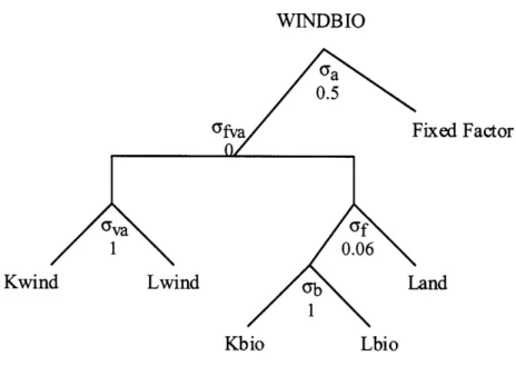
To represent large scale renewables, I created two new renewable backstop technologies: large scale wind with biomass backup and large scale wind with NGCC backup. Unlike regular wind, solar, and biomass, large scale wind with biomass or NGCC backup are modeled as perfect substitutes for other electricity because the backup makes up for intermittency. The elasticity of substitution does not create a gradually increasing cost of production as the share of these two technologies increases in the generation mix. The additional costs for large scale wind
(transmission and storage or backup) are incorporated into the markup costs of the new technologies as is explained below.
The main drawback of renewable technologies like wind and solar is their intermittency. As wind and solar increase in scale, making up a larger portion of electricity generation,
intermittency becomes even more of an issue. It becomes necessary for these large scale renewable operations to have a reliable backup source of generation.5 I focus on wind as it the most rapidly expanding renewable and an RPS would likely favor wind, as it has in states with an RPS. It is often assumed that wind can make up a significant portion of electricity generation without threatening the reliability of electricity with its intermittence if turbines are
geographically distributed across large areas with low wind correlation. However, there are times when the wind is still for hours or even days at a time over expansive regions (Joint Coordinated
System Plan). Such occurrences would be devastating to an electricity system relying on wind for a significant portion of generation. While spreading out wind sites reduces the number of hours with low or zero wind, there is still an effective limit imposed by intermittency. Regardless
of how much wind capacity is built, there are still periods when the wind does not blow and backup capacity must be utilized to meet the load. This may create the need for an installed
capacity of backup generation of 1 KW for every KW of installed capacity of wind. Even though these backup plants would rarely operate, they would need to be capable of replacing all wind generation in the case of a wind block.
A study by Decarolis and Keith (2006) on large scale wind found natural gas to be crucial to a large-scale wind system. They used an optimizing model that minimizes the average cost of electricity by adjusting wind capacity at various sites, a storage system, and gas turbines to meet time varying load under a carbon tax. They found that as the level of wind increased (as the carbon tax increased), the installed gas capacity remained equal to the maximum load so as to be able to meet peak demand if there was no wind. At high levels of wind penetration, the gas turbines effectively acted as capacity reserve that ramped to complement the time-varying wind. There are options other than gas that could also serve as the reserves. The point is that large scale wind needs to be accompanied by a nearly equal capacity of a backup. A storage system is an 5 Increasing the price responsiveness of demand is another potential method for managing intermittency. Residential
customers could be provided with real-time monitors that track energy consumption and price. However, studies have shown demand response to be weak, particularly at the short timescales of economic dispatch (Matsukawa, 2004). Another more effective option is for customers to allow system operators to control appliance loads.
alternative to backup capacity. However, compressed air, pumped hydro, batteries, and other technologies are prohibitively expensive at this time, making backup capacity more likely.
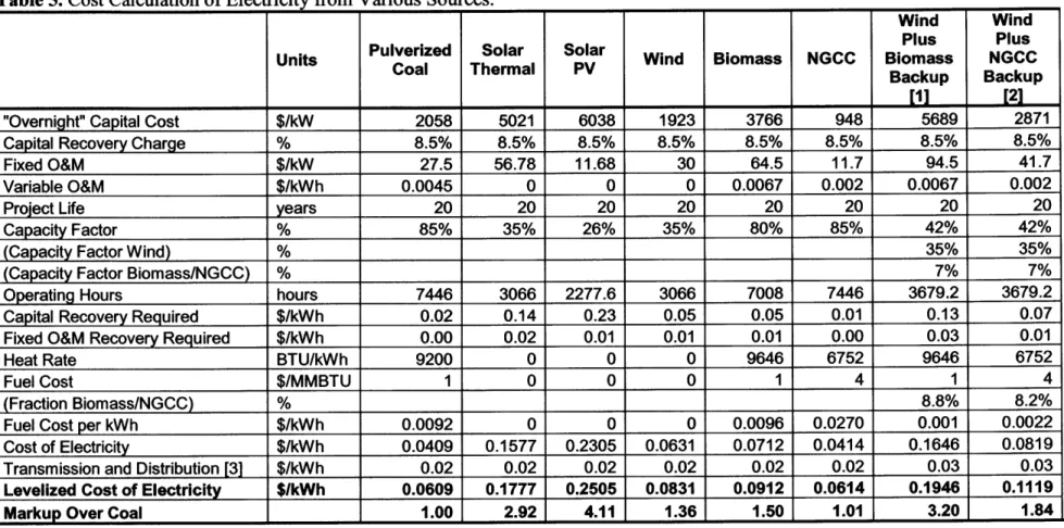
To represent large scale wind with backup capacity in the EPPA model, I created two new renewable technologies: large scale wind with biomass backup and large scale wind with NGCC backup. To do so I calculated the levelized cost of electricity from pulverized coal, wind,
biomass, NGCC, wind plus biomass backup and wind plus NGCC backup (see Table 5). Overnight capital and fixed and variable operation and maintenance (O&M) costs were taken from EIA data (2009). For simplicity, all plants were assumed to have a 20 year lifetime. Capacity factors for the traditional plants, heat rate, and fuel costs were taken from a study conducted by Lazard Ltd. (Lazard, 2008). The capital recovery rate of 8.5% was calculated as the rate that gives the constant capital recovery necessary each year over the life of the plant in
order to recover capital costs, taking into account inflation and discounting.6
For the wind with backup it is assumed that for every KW installed capacity of wind there is one KW installed capacity of backup (either biomass or NGCC). The backup allows the
combined plant to be fully reliable because whenever the wind is not blowing demand can still be met through the backup. It is assumed that the backup is only needed 7% of the time (for the rare occurrences when there is no wind). Since the wind operates 35% of the time, this gives a combined capacity factor of 42%. Capital, O&M and fuel costs of a wind plant are combined with those of a biomass or NGCC plant in the levelized cost calculation for wind with backup.
The calculation provides a levelized cost of electricity of 4.1 cents per kWh for pulverized coal, 15.8 cents per kWh for solar thermal, 23.1 cents per kWh for solar photovoltaic (PV), 6.3 cents per kWh for wind, 7.1 cents per kWh for biomass, 4.1 cents per kWh for NGCC, 16.5 cents per kWh for wind with biomass backup, and 8.2 cents per kWh for wind with NGCC backup. As discussed in Chapter 3, we also need to account for the costs of transmission and distribution. I assume an additional $0.02 per kWh for regular electricity sources and an additional $0.03 per kWh for large scale wind plus biomass and large scale wind plus NGCC. The $0.02 per kWh comes from work by McFarland (2002). The extra $0.01 for large scale wind with backup is assumed to account for the fact that such large scale wind production will be predominately located in the middle of the country at the best wind sites, which is far away from electricity demand which is largely concentrated on the coasts. For example, Wyoming is a prime site for
Table 5. Cost Calculation of Electricity from Various Sources.
Wind Wind Plus Plus Units Pulverized Solar Solar Wind Biomass NGCC Biomass NGCC
Coal Thermal PV Backup Backup
"Overnight" Capital Cost $/kW 2058 5021 6038 1923 3766 948 5689 2871
Capital Recovery Charge % 8.5% 8.5% 8.5% 8.5% 8.5% 8.5% 8.5% 8.5%
Fixed O&M $/kW 27.5 56.78 11.68 30 64.5 11.7 94.5 41.7
Variable O&M $/kWh 0.0045 0 0 0 0.0067 0.002 0.0067 0.002
Project Life years 20 20 20 20 20 20 20 20
Capacity Factor % 85% 35% 26% 35% 80% 85% 42% 42%
(Capacity Factor Wind) % 35% 35%
(Capacity Factor Biomass/NGCC) % 7% 7%
Operating Hours hours 7446 3066 2277.6 3066 7008 7446 3679.2 3679.2 Capital Recovery Required $/kWh 0.02 0.14 0.23 0.05 0.05 0.01 0.13 0.07
Fixed O&M Recovery Required $/kWh 0.00 0.02 0.01 0.01 0.01 0.00 0.03 0.01
Heat Rate BTU/kWh 9200 0 0 0 9646 6752 9646 6752
Fuel Cost $/MMBTU 1 0 0 0 1 4 1 4
(Fraction Biomass/NGCC) % 8.8% 8.2%
Fuel Cost per kWh $/kWh 0.0092 0 0 0 0.0096 0.0270 0.001 0.0022
Cost of Electricity $/kWh 0.0409 0.1577 0.2305 0.0631 0.0712 0.0414 0.1646 0.0819
Transmission and Distribution [3] $/kWh 0.02 0.02 0.02 0.02 0.02 0.02 0.03 0.03
Levelized Cost of Electricity $/kWh 0.0609 0.1777 0.2505 0.0831 0.0912 0.0614 0.1946 0.1119
Markup Over Coal 1.00 2.92 4.11 1.36 1.50 1.01 3.20 1.84
[1] For calculation purposes we assume a combined wind and
installed capacity of wind so that when the wind is not blowing the biomass operates 7% of the time.
[2] For calculation purposes we assume a combined wind and
installed capacity of wind so that when the wind is not blowing the NGCC operates 7% of the time.
biomass plant where there is 1 KW installed capacity of biomass for every 1 KW
a full kWh can be produced. We assume the wind operates 35% of the time and
NGCC plant where there is 1 KW installed capacity of NGCC for every 1KW
a full kWh can be produced. We assume the wind operates 35% of the time and
[3] Transmission and distribution costs are assumed to be 2 cents per kWh for existing technologies and 3 cents per kWh for new large scale