User’s Guide to GEOMAGIA50.v3:
2. Sediment Database
Maxwell C. Brown1,∗, Fabio Donadini2, Andreas Nilsson3,4, Sanja Panovska5, Ute Frank1, Kimmo Korhonen6, Maximilian Schuberth7,8, Monika Korte1, Catherine G. Constable5
1Helmholtz-Zentrum Potsdam, Deutsches GeoForschungsZentrum, Telegrafenberg, 14473 Potsdam, Germany 2Department of Earth Sciences, University of Fribourg, Chemin du Mus´ee 6, 1700 Fribourg, Switzerland
3Geomagnetism Laboratory, Department of Earth, Ocean and Ecological Sciences, University of Liverpool, Liverpool, L69 7ZE, UK
4Now at Department of Geology, Quaternary Sciences, Lund University, S¨olvegatan 12, 223-62 Lund, Sweden
5Institute of Geophysics and Planetary Physics, Scripps Institution of Oceanography, University of California, San Diego, La Jolla, California, USA
6Geological Survey of Finland (GET), P.O. Box 96 (Betonimiehenkuja 4), FI-02151 Espoo, Finland 7Institute of Earth and Environmental Science, University of Potsdam, 14476 Potsdam, Germany
8Now at Faculty of Civil Engineering and Geosciences, Delft University of Technology, 2628 CN Delft, Netherlands ∗Contact at[email protected]
T
his guide is the second of a pairde-scribing the function of the GEOMA-GIA50.v3 database. The first accompa-nies Brown et al.(2015a) (referred to here as B15a). This guide constitutes the Support-ing Information associated with Brown et al. (2015b), hereafter referred to as B15b.
Contents
1 Guide to the function of the sediment web
page 1
1.1 Query form . . . 1
1.1.1 Query, download and model options . . . 3
1.1.2 Age constraints . . . 3
1.1.3 Geographic constraints . . . . 3
1.1.4 Advanced querying options . 5 1.2 Navigation menu options for sediments 6 2 Description of database output 6
List of Figures
1 Sediment query form . . . 24 Geographic autocomplete/dropdown menus . . . 3
2 Download tab . . . 4
3 Results tabs . . . 4
5 Advanced query panel . . . 5
6 Google map of sediment locations. . 7
List of Tables
S1 Fields common to two or more results tables . . . 8S2 ‘Individual (Specimen/Stratigraphic) Level Sediment’ unique field headers 9 S3 ‘Processed (Averaged/Smoothed) Sediment’ unique field headers . . . 9
S4 ‘Radiocarbon Age’ unique field headers 10 S5 ‘General Age’ unique field headers . 10 S6 ‘Reconstructed Paleomagnetic Time Series’ unique field headers . . . 11
1 Guide to the function of the
sediment web page
The operation of the query form and web pages listed in the navigation bar are described in the following sections.
1.1 Query form
The sediment query form (Fig. 1) can be accessed at http://geomagia.gfz-potsdam.de/ geomagiav3/SDquery.phpor through the ‘Sediment query form’ link in the left navigation menu. The main functions of this form are briefly described.
Figure 1: Initial state of the sediment query form after the user has selected the ‘Sediment query form’ link from
the left navigation menu on the GEOMAGIA50 home page or entered http: // geomagia. gfz-potsdam. de/ geomagiav3/ SDquery. php into a browser’s address bar.
1.1.1 Query, download and model options
The options under this heading are described in sec-tion ‘Query, download and model opsec-tions’ in B15b. Selecting a ‘View’ checkbox under ‘Query, Download and Model Options’ will generate an HTML table of data in a new tab in the browser once the query has been executed. Choosing a ‘Download’ checkbox produces a link to download a .CSV file in a new tab in the browser (Fig. 2). By default all checkboxes next to the data types to query are checked. The user can check ‘View’ by itself; however, if the user selects ‘Download’ then ‘View’ will also be selected. The relational tables beneath the online tables (Fig. 3) are necessary to interpret the IDs in the .CSV files.
1.1.2 Age constraints
Temporal constraints are set by one of four options, which the user chooses by selecting a radio button (Fig.1). Selecting ‘None’ allows the user to retrieve whatever part of a time series lies between -50 yr. BP (2000 AD) and 50,000 yr. BP. The ‘None’ option also recovers data for which no age control is explicitly stated. In contrast, selecting ‘Age between’, ‘Age <’ or ‘Age >’ will select only data coupled with an age. All text entry boxes are deactivated (boxes appear grey and clicking on the box does not allow text entry; the appearance may vary with browser and operating system) until a radio button is selected.
1.1.3 Geographic constraints
The user has the choice of seven options to constrain the location or range of locations over which the database will query (Fig. 1). Choices are controlled by radio buttons. As with ‘Age constraints’, text entry boxes are only active when the associated radio button is selected. Only the entry in the text box with the activated radio button will be parsed into the database query.
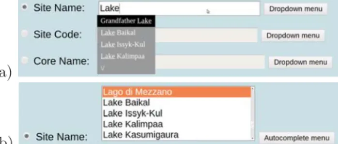
With the exception of ‘None’ and ‘Custom’ two methods of location entry are possible: ‘Autocom-plete menu’ or ‘Dropdown menu’ (Fig. 4). The de-fault option when the query form loads is the au-tocomplete menu. The auau-tocomplete menu allows the user to manually type an entry or part of an entry into the text box, which is activated when the radio button is selected (as with ‘Age constraints’). When text is entered an array containing all entries related to the radio button selected is queried and matches are progressively displayed on the screen as a list. For example, selecting the ‘Location Name’ radio button and entering ‘Lake’ will produce a list
(a)
(b)
Figure 4: Alternative methods of selecting geographic
constraints using (a) an autocomplete menu or (b) a dropdown menu.
of all the locations that include ‘Lake’ (Fig.4a). The case is important. The list is truncated to the first four entries in alphabetical order, but further entries can be revealed by clicking the down arrow below the fourth entry. An entry from this list can then be selected by clicking on the desired location. This will automatically fill in the entry box. Alternatively, clicking on ‘Dropdown menu’ allows the user to re-turn a full list of the entries for a certain category of geographic constraint (Fig. 4b). Entries are listed alphabetically and the user can scroll through all entries using the righthand scroll bar or can enter a letter of the alphabet to jump to the first entry starting with this letter. The entry is selected by clicking on the name of the geographic constraint. A colored bar remains behind the selected entry.
Selecting the ‘None’ radio button will query every location in the database. This will result in a global search over the past 50 ka and will return every entry in the database. No model output will be chosen when ‘None’ is selected.
‘Continent/Ocean’ will query all locations lying in one of the seven commonly defined continents or five commonly defined oceans. This option will generate no model output, even if one or more ‘Model options’ checkboxes are selected. The spatial range covered by each entry is so large that producing model output for a single arbitrary location within a continent or ocean when the structure of the field may vary significantly within these areas is uninformative.
‘Country/State/Region/Sea’ queries politically de-fined land masses or water bodies. For larger coun-tries, e.g., USA, entries are given as states, etc, where appropriate. Model output will be produced for the geographic center of selected location.
‘Location Name’ contains all lake names and ma-rine locations. For mama-rine locations it is more com-mon to refer to the drilling site, e.g., an ODP site number. In such cases we chose the broad location at which the core was taken, e.g., ODP Site 919
Figure 2: The appearance of the ‘Download Material’ tab. The left column lists all possible categories of data that
can be downloaded. The right column gives the user the option to download data files via hyperlinks, depending on whether the query returned any results for a particular category of data.
Figure 3: The appearance of the results web page showing the six on-page tabs. The first few output columns of the
‘Individual Specimen/Stratigraphic Level Sediment Tables’ tab are shown for an example query from Israel, along with two examples of relational tables (‘Location Names’ and ‘References’) accompanying this query. The underlined entries are hyperlinks.
(Channell,2006) was located in the Irminger Basin. More familiar coring site numbers are listed under ‘Core Name’.
Every location name is assigned a three letter location code as used in the CALSxk series of models (see Table 1. in Korte et al., 2011). Once known, by entering this code in ‘Location Code’ the user can quickly query a location, rather than scrolling through a list of locations or typing in part of or a full location name. This is especially efficient for repeating queries for a certain location. The list of location codes will increase through time as more locations are added to the database and will exceed those given in Korte et al. (2011). The location name corresponding to a location code can be found when the map of sediment locations is opened in maps.google.com (see section 1.2).
‘Core Name’ queries for the name of core as listed in a publication. Only one core can be queried at a time. For lake locations multiple cores are often taken and data from only one core may be of interest. This is the preferred option for searching for marine core data and includes, e.g., IODP, ODP and MD Site numbers in the name.
‘Custom’ is the most flexible geographic constraint and is particularly useful for regional studies, e.g., for retrieving data from only the Southern Hemisphere or from a geographic area which crosses political bor-ders, such as the area surrounding the Mediterranean. Longitude can be entered as positive or negative de-grees east (between -180◦ E and 180◦ E or 0◦ and 360◦ E), with a range no greater than 360◦. Error messages will appear if the this range is exceeded, if the two longitudes have the same value or if the longitudes lie outside -180◦ E to 360◦ E. Latitude errors are given when values greater than 90◦N or less than -90◦N are entered, or when the same value is entered in both boxes.
1.1.4 Advanced querying options
Advanced query options are accessed by click on the plus sign next to the section header (Fig. 1). Once clicked the web page expands vertically and reveals three boxes containing additional querying options. The default setting is to query all data (Fig. 5a). Individual paleomagnetic and rock magnetic data are set to ‘Non-specific’ and all general age options are selected. This will return the same results as if advanced querying options boxes were not revealed. The two query boxes on the left hand side allow the user to refine their search of the individual pa-leomagnetic and rock magnetic data. ‘Directions’,
(a)
(b)
Figure 5: Examples of the advanced query form: (a)
with default options and (b) with refined data querying and output options.
‘ Relative paleointensity’ and ‘Rock magnetic’ data are selected by clicking between radio buttons. If the ‘Rock magnetic’ radio button is selected, then a series of check boxes are revealed under the heading ‘Specific rock magnetic’. These allow the user to
further refine their search (Fig.5b).
‘General age data’ options are chosen by selecting the check boxes on the right side of the screen. As with the rock magnetic options, multiple choices can be made (Fig. 5b).
‘Output options’ allows the user to choose which data are written to the screen and saved on download. There are two options: (1) ‘All columns’ and (2) ‘Selected parameter columns’. ‘All columns’ outputs every column of data for an entry that contains one of the advanced querying options selected. For example, if ‘All columns’ is selected in conjunction with ‘Rock magnetic’, and only the ‘Hysteresis parameters’ check box is chosen, then all hysteresis columns (Mr, Mrs, Hc and Hcr) are output for entries containing one of these parameters, along with all other fields (NRM, susceptibility, etc).
If ‘Selected parameter columns’ is chosen only the fields for which the data exist are output. For the hysteresis example, Mr, Mrs, Hc and Hcr and the location metadata are shown as output. ‘Output options’ works with both individual paleomagnetic
and rock magnetic options and general age data. Default options can be reinstated by clicking the ‘Reset all advanced query options’ button. Closing the ’Advanced querying options’ panel by clicking on the minus symbol at the top of panel (as in the default state when the sediment query form loads) deactivates all options within the panel; however, does not reset them. Therefore if the panel is again opened previous selected options are again visible and active.
1.2 Navigation menu options for sediments The ‘Complete sediment data sets’ web page (http://geomagia.gfz-potsdam.de/complete_ sediment_data.php) opens a new web page con-taining .CSV files of the five results tables. The amount of individual data is prohibitively large to print to the screen efficiently when no constraints are chosen. When a user queries the database without selecting any constraints, they are redirected to this web page. In addition, it contains a summary of all identification numbers (section ‘Metadata tables and identification numbers’ in B15b). All files can be downloaded at once as a .zip file. The version of the tables are denoted with the date of creation at the end of the file name.
The ‘Glossary of IDs’ web page (http: //geomagia.gfz-potsdam.de/ID_glossary.php) lists all metadata tables and the IDs found within any of the results tables. The metadata table names are listed at the top of the page. Each table is a hyperlink. Clicking on the metadata table name takes the user to the appropriate metadata table, e.g., clicking on ‘Location Codes for Sediments’ takes the user to a table containing the three letter short code of all the location names accompanied by their full name. The tables shown on this page are related to the both the sediment database and the archeomagnetic and volcanic database (B15a). The webpage automatically updates as new data are supplemented to the metadata tables, e.g., if a new location and code is added, this will appear in the ‘Location Codes for Sediments’ table (http://geomagia.gfz-potsdam.de/ID_ glossary.php#SedLocCode).
The ‘Available sediment studies’ web page (http://geomagia.gfz-potsdam.de/ sedimentstudies.php) contains a full refer-ence list for studies included in the database. The number of references currently within the database is listed above the reference table header. This is calculated for the number of references, not the
number of reference groups. The references can be ordered by ID, Group ID (section ‘Metadata’ in B15b), first author surname, year of publication and journal. The IDs and Group IDs are the same as those listed under ‘Reference ID’ and ‘Reference Group ID’ in the five results tables (Fig.3). Every reference is accompanied by either a hyperlinked DOI or a hyperlink to an online holding of the source material. The final column lists hyperlinks to the MagIC database, if data from a particular reference are also stored within the MagIC database (http://earthref.org/MAGIC/). This is the case for data used in the SEDPI06 compilation of Tauxe
and Yamazaki (2007). Two search boxes allow the
user to search for references based on author or by words contained with the title of a publication. The author search will search though all authors and coauthors.
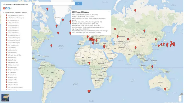
The ‘Map of sediment locations’ web page (http: //geomagia.gfz-potsdam.de/sedimentmap.php) takes the user to a web page containing a Google map that shows the locations of all sediment locations currently uploaded to the database (Fig.6). Each location is marked with a balloon. Clicking on the balloon reveals basic location and core level information. At the bottom of the map there is a link to open the map on themaps.google.com web page. This expands the map and gives the user a list of all locations on the left hand side of the map.
2 Description of database output
This section contains six tables (Tables S1 to S6) describing the output headers of the online tables and the .CSV data files. The model .TXT files are described in Additional File 1 of B15a.
References
Brown, M. C., F. Donadini, M. Korte, A. Nilsson, K. Korhonen, A. Lodge, S. N. Lengyel, and C. G. Constable (2015a), GEOMAGIA50.v3: 1. general structure and modifications to the archeological and volcanic database, submitted to Earth Planets
Space.
Brown, M. C., F. Donadini, U. Frank, S. Panovska, A. Nilsson, K. Korhonen, M. Schuberth, M. Korte, and C. G. Constable (2015b), GEOMAGIA50.v3: 2. a new paleomagnetic database for lake and ma-rine sediments, submitted to Earth Planets Space.
Figure 6: Google map of sediment locations included in the GEOMAGIA50 database (December 2014) opened in
maps.google.com.
Channell, J. E. T. (2006), Late Brunhes polarity ex-cursions (Mono Lake, Laschamp, Iceland Basin and Pringle Falls) recorded at ODP Site 919 (Irminger Basin), Earth Planet. Sci. Lett., 244, 378–393, doi:10.1016/j.epsl.2006.01.021.
Kirschvink, J. L. (1980), The least-squares line and plane and the analysis of palaeomagnetic data,
Geophys. J. R. astr. Soc., 62, 699–718, doi:10.1111/
j.1365-246X.1980.tb02601.x.
Korte, M., C. Constable, F. Donadini, and R. Holme (2011), Reconstructing the Holocene geomagnetic field, Earth Planet. Sci. Lett., 312, 497–505, doi: 10.1016/j.epsl.2011.10.031.
Piper, J. D. A. (1989), Palaeomagnetism, in
Geomag-netism, edited by J. A. Jacobs, vol. 3, Academic
Press, London.
Tauxe, L., and T. Yamazaki (2007), 5.13 - pale-ointensities, in Treatise on Geophysics, edited by G. Schubert, pp. 509 – 563, Elsevier, Amsterdam, doi:10.1016/B978-044452748-6.00098-5.
Online table header CSV file header Description Results tables
Age (yr. BP) Age[yr.BP] Age in years BP to nearest year. 1,2,5
Age-Depth Model ID AgeDepthModelID IDs of procedures used to transfer depth to age.
http://geomagia.gfz-potsdam.de/ID_glossary.php#AgeModelID 1,2,5 Calib. dataset ID CalibDatasetID ID of the dataset used to calibrate for atmospheric variations in14C through time.
http://geomagia.gfz-potsdam.de/ID_glossary.php#C14DataSet 3,5 Calibrated? AgeCalib If14C ages were calibrated in the construction of the time series
(Y=yes; N=No; NA=no14C ages used). 1,2
Comp. Depth (cm) CompDepth[cm] Composite or final depth scale after all correlations and adjustments (cm). 1,2,5 Comp. Depthmin(cm) CompDepthMin[cm] Minimum (shallowest) composite depth reported (cm). 3,4 Comp. Depthmax(cm) CompDepthMax[cm] Maximum (deepest) composite depth reported (cm). 3,4 Core Depthmin(cm) CoreDepthMin[cm] Minimum (shallowest) raw depth reported (cm). 3,4 Core Depthmax(cm) CoreDepthMax[cm] Maximum (deepest) raw depth reported (cm). 3,4 Core ID CoreID Name of core given in publication. If cores have been combined and it is
not possible to reconcile the original name then the core is labeled ‘Stack’. 1,3,5 DecadjID DecAdjID ID(s) of the adjustments made to declination.
http://geomagia.gfz-potsdam.de/ID_glossary.php#DecAdj 1,2,5 IncadjID IncAdjID ID(s) of the adjustments made to inclination.
http://geomagia.gfz-potsdam.de/ID_glossary.php#IncAdj 1,2,5 Environ. ID EnvironID Depositional environment ID.
http://geomagia.gfz-potsdam.de/ID_glossary.php#EnvironID 1,2 Notes ID NotesID Additional descriptive notes not accommodated by other entries.
http://geomagia.gfz-potsdam.de/ID_glossary.php#NoteID 1,2,3,4,5 NRM/ARM NRM ARM The ratio of natural remanent magnetization (NRM) to anhysteretic
remanent magnetization (ARM) used as a proxy for relative paleointensity (RPI). 1,2,5 NRM/k NRM k The ratio of natural remanent magnetization (NRM) to susceptibility (k)
used as a proxy for relative paleointensity (RPI). 1,2,5 NRM/IRM NRM IRM The ratio of natural remanent magnetization (NRM) to isothermal
remanent magnetization (IRM) used as a proxy for relative paleointensity (RPI). 1,2,5
±σ yr. Sigma[yr.] Uncertainty on an age. 3,4
Reference Group ID ReferenceGroupID ID for a set of references from which data were obtained.
http://geomagia.gfz-potsdam.de/sediment_studies.php 1,2,3,4,5 RPIprefID RPIprefID ID of the author’s preferred RPI normalization method.
http://geomagia.gfz-potsdam.de/ID_glossary.php#RPIID 1,2
Sample Code SampleCode Laboratory sample code. 3,4
σID SigmaID ID of the type of uncertainty.
http://geomagia.gfz-potsdam.de/ID_glossary.php#RPIErrorID 2,4,5
σNRM/ARM Sigma[NRM ARM] Uncertainty on NRM/ARM. 1,2,5
σNRM/ARMID Sigma[NRM ARM]ID Type of uncertainty for NRM/ARM.
http://geomagia.gfz-potsdam.de/ID_glossary.php#RPIErrorID 1,2,5
σNRM/IRM Sigma[NRM IRM] Uncertainty on NRM/IRM. 1,2,5
σNRM/IRMID Sigma[NRM IRM]ID Type of uncertainty for NRM/IRM.
http://geomagia.gfz-potsdam.de/ID_glossary.php#RPIErrorID 1,2,5
σNRM/k Sigma[NRM k] Uncertainty on NRM/k. 1,2,5
σNRM/kID Sigma[NRM k]ID Type of uncertainty for NRM/k.
http://geomagia.gfz-potsdam.de/ID_glossary.php#RPIErrorID 1,2,5 σVDM,VADM Sigma[VDM VADM] Uncertainty on VDM or VADM (see ‘VDM or VADM’). 1,2 σVDM,VADMID Sigma[VDM VADM]ID Type of uncertainty for VDM or VADM.
http://geomagia.gfz-potsdam.de/ID_glossary.php#RPIErrorID 1,2 Location Code LocationCode Three letter location code (see section1.1.3).
http://geomagia.gfz-potsdam.de/ID_glossary.php#SedLocCode 1,2,3,4,5 Lat. (◦) Lat[deg.] Location or core latitude (◦N). Cross checked against Google Earth WGS84 datum.
If erroneous then corrected and a note given in ‘Notes ID’. 1,2,3,4,5 Lon. (◦) Lon[deg.] Location or core longitude (◦E). Cross checked against Google Earth WGS84 datum.
If erroneous then corrected and a note given in ‘Notes ID’. 1,2,3,4,5 Source ID SourceID ID of source of data (see section ’Data sources’ in B15b).
http://geomagia.gfz-potsdam.de/ID_glossary.php#UpModID 1,2,3,4,5
Upload Date UploadDate Date of upload to the database. 1,2,3,4,5
Uploader Uploader Initials of person responsible for upload of data. 1,2,3,4,5 VDM or VADM VDM RPI converted to a virtual dipole moment (VDM) or
virtual axial dipole moment (VADM) x1022Am2. 1,2
UID UID Unique identification number of an entry 1,2,3,4,5
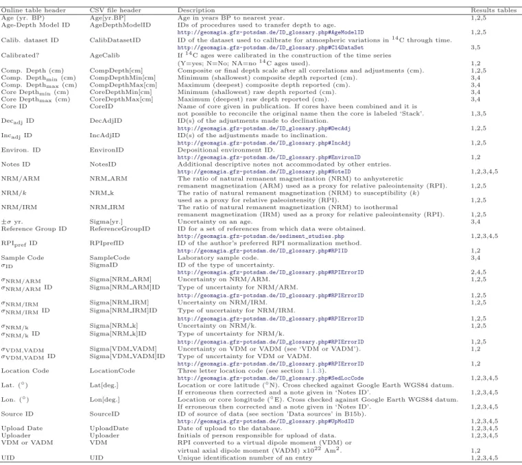
Table S1: Fields common to two or more results tables. Arranged in alphabetical order. IDs are numbers in
corresponding relational tables. These are given below the online tables and linked via hyperlinks from the ID. ‘Results tables’ lists the tables in which the headers appear: 1 = ‘Individual (Specimen/Stratigraphic) Sediment’; 2 = ‘Processed (Averaged/Smoothed) Sediment’; 3 = ‘Radiocarbon Age’; 4 = ‘General Age’; 5 = ‘Reconstructed Palaeomagnetic Time Series’.
Online table header CSV file header Description
Sed. Rate (cm/ka) SedRate[cm/ka] Sedimentation rate in cm/ka for specific depth ranges or an average for the core. Specimen ID SpecimenID ID of the specimen type, e.g., for standard cubes or u-channels.
http://geomagia.gfz-potsdam.de/ID_glossary.php#SpecID
Core Depth (cm) CoreDepth[cm] Raw depth of core measurements before correlation of cores or adjustments to depth (cm).
Dir. ID DirID ID of the method used to determine the direction of the characteristic remanent magnetization (ChRM).
http://geomagia.gfz-potsdam.de/ID_glossary.php#DirID
Min. AF Demag. (mT) MinAFDemag[mT] Minimum alternating field (AF) (mT) used to isolate the ChRM. Max. AF Demag. (mT) MaxAFDemag[mT] Maximum AF (mT) used to isolate the ChRM.
Decraw(◦) DecRaw[deg.] Declination (◦) before any corrections for, e.g., core rotation or azimuth. Incraw(◦) IncRaw[deg.] Inclination (◦) before any corrections, e.g., sub-vertical penetration.
MAD (◦) MAD[deg.] Maximum angular deviation determined using principal component analysis (Kirschvink,1980). Decadj(◦) DecAdj[deg.] Final declination (◦) after adjustments considered.
Incadj(◦) IncAdj[deg.] Final inclination (◦) after adjustments considered.
Susc. Susc Susceptibility.
Factor Factor Multiplicative factor (e.g., x10−3) for the preceding value. Unit Unit Measurement unit of susceptibility for the preceding value. NRMrpi NRM RPI NRM value used in the calculation of RPI.
NRMrpiDemagMin(mT) NRM RPI Demag Min[mT] Minimum AF (mT) used to isolate the NRM value in NRMrpi. Given if a fit through NRM-ARM or NRM-IRM spectra used. NRMrpiDemagMax(mT) NRM RPI Demag Max[mT] Maximum AF (mT) used to isolate the NRM value in NRMrpi.
Given in isolation if a blanket demagnetization used. NRMrm NRM RM NRM value used in rock magnetic analysis. ARMrpi ARM RPI ARM value used in the calculation of RPI.
ARMrpiDemagMin(mT) ARM RPI Demag Min[mT] Minimum AF (mT) used to isolate the ARM value in ARMrpi. Given if a fit through NRM-ARM spectra used.
ARMrpiDemagMax(mT) ARM RPI Demag Max[mT] Maximum AF (mT) used to isolate the ARM value in ARMrpi. Given in isolation if a blanket demagnetization used. ARMrm ARM RM ARM value used in rock magnetic analysis. IRMrpi IRM RPI IRM value used in the calculation of RPI.
IRMrpiDemagMin(mT) IRM RPI Demag Min[mT] Minimum AF (mT) used to isolate the IRM value in IRMrpi. Given if a fit through NRM-IRM spectra used.
IRMrpiDemagMax(mT) IRM RPI Demag Max[mT] Maximum AF (mT) used to isolate the IRM value in IRMrpi. Given in isolation if a blanket demagnetization used. IRMrm IRM RM IRM value used in rock magnetic analysis.
bIRMrm bIRM RM Backfield IRM (bIRM) value.
BIRM(T) IRM B[T] Applied field (T) used to induce an IRM. BbIRM(T) bIRM B[T] Applied field (T) used to induce an bIRM. HIRM HIRM Hard isothermal remanence (IRM+(-bIRM)/2.
S-ratio S-ratio Value of S-ratio.
S-ratio ID S-ratioID ID of type of S-ratio calculation.
http://geomagia.gfz-potsdam.de/ID_glossary.php#SRID
MDFNRM(mT) MDF NRM[mT] Median destructive field of NRM (mT). MDFARM(mT) MDF ARM[mT] Median destructive field of ARM (mT). MDFIRM(mT) MDF IRM[mT] Median destructive field of IRM (mT).
Mr Mr Remanence of saturation magnetization determined from hysteresis. Ms Ms Saturation remanent magnetization determined from hysteresis.
Hc Hc Coercivity.
Hcr Hcr Backfield coercivity.
Mineral ID MineralID IDs of magnetic minerals present, as interpreted by author.
http://geomagia.gfz-potsdam.de/ID_glossary.php#MagMin
Dating Method ID DatingMethodID IDs of methods used to date sediment at a specific depth.
http://geomagia.gfz-potsdam.de/ID_glossary.php#DatMethod
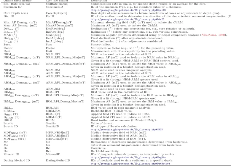
Table S2: Fields headers and descriptions unique to the ‘Individual (Specimen/Stratigraphic) Level Sediment’ online
table and .CSV file. Arranged by order of appearance in table. See Table S1for further details.
Online table header CSV file header Description
Ncores N Cores Number of cores combined in the averaging/smoothing analysis.
Core Names CoreNames Names of cores used to create an averaged/smoothed or reconstructed record. Smoothing Level SmoothingLevel Whether smoothing is by strata or time.
Nspecimens N SpecimensSmoothed Number of specimens or measurements used to create each averaged/smoothed value. Dir. Smoothing Type ID DirSmoothingTypeID ID of type of averaging/smoothing procedure for directional data.
http://geomagia.gfz-potsdam.de/ID_glossary.php#SmoothID
Dec. (◦) Dec[deg.] Averaged/smoothed declination (◦). Inc. (◦) Inc[deg.] Averaged/smoothed inclination (◦).
σDec(◦) SigmaDec[deg.] Uncertainty of averaged/smoothed declination. If uncertainty is given asα95.
the standard deviation is shown as: (81/140cos(I))α95where I=inclination (Piper,1989) (◦). σInc(◦) SigmaInc[deg.] Uncertainty of declination. If uncertainty is given asα95the standard deviation.
is shown as: (81/140)α95(Piper,1989) (◦).
DecID DecID ID(s) of the adjustments made to declination before averaging/smoothing.
http://geomagia.gfz-potsdam.de/ID_glossary.php#DecID
IncID IncID ID(s) of the adjustments made to inclination before averaging/smoothing.
http://geomagia.gfz-potsdam.de/ID_glossary.php#IncID
RPI Smoothing Type ID RPISmoothingTypeID ID of the method used to averaging/smoothing RPI data.
http://geomagia.gfz-potsdam.de/ID_glossary.php#SmoothID
Pmag Type ID PmagTypeID ID of type of measurement made to obtain raw data before averaging/smoothing.
http://geomagia.gfz-potsdam.de/ID_glossary.php#SedSampID
Dating Method ID DatingMethodID IDs of dating methods used in the creation of an age-depth model applied across all depths.
http://geomagia.gfz-potsdam.de/ID_glossary.php#DatMethod
Table S3: Field headers and descriptions unique to the ‘Processed (Averaged/Smoothed) Sediment’ online table and
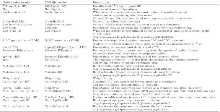
Online table header CSV file header Description
14C age (yr. BP) 14CAge[yr.BP] Uncalibrated14C age in years BP.
Nσ NumSigma Number of standard deviations.
Author Accept? AuthorAccept Whether author accepted date in construction of age-depth model used to make a paleomagnetic time series.
(Y=yes; N=no; NA=not associated with a paleomagnetic time series). Libby Half Life LibbyHalfLife Value of the Libby Half Life used.
Lab Error Multiplier LabErrorMultiplier Value of a laboratory error multiplier if stated in publication. Lab Code LabCode Laboratory code as listed in the compilation of www.radiocarbon.org.
Lab Type ID LabTypeID Whether laboratory is conventional (Conv.), accelerator mass spectrometer (AMS) or not listed.
http://geomagia.gfz-potsdam.de/ID_glossary.php#C14LabCode
δ13C (per mil w.r.t PDB) D13C[permil.w.r.t.PDB] Degree of isotopic fractionation between12C and13C in per mil
relative to the PDB standard ratio, used to correct the measurement of14C. ±σ (δ13C) Sigma[D13Cpermil.w.r.t.PDB] Uncertainty at one standard deviation ofδ13C.
Reservoir Effect (yr.) ReservoirEffect[yr.] Estimate of the offset in years resulting from the uptake of carbon from a source (or reservoir) other than atmospheric carbon.
±σ yr. (RE) ReservoirEffectError[yr.] Uncertainty at one standard deviation of the reservoir effect.
ΔR DeltaR[yr.] The regional difference (in years) from the average global marine reservoir correction. Applied to marine specimens only.
Material Type ID1 MaterialID1 ID of specific material type used for dating.
http://geomagia.gfz-potsdam.de/ID_glossary.php#DatMatID1
Material Type ID2 MaterialID2 ID of a broader (vague) category of materials used for dating.
http://geomagia.gfz-potsdam.de/ID_glossary.php#DatMatID2
Weight (mg) Weight[mg] Weight in mg.
Calib. age (yr. BP) CalibAge[yr.BP] Measured14C age calibrated for variations in atmospheric and marine carbon through time. In years BP.
±σ yr. (calib. age) Sigma[yr.] Uncertainty on the calibrated age if given as a standard deviation (in years). Min. calib. age (yr. BP) MinCalibAge[yr.BP] Minimum calibrated age in years BP if ages reported as minimum and maximum ages
(e.g., if a probability method was used for calibration).
Max. calib. age (yr. BP) MaxCalibAge[yr.BP] Maximum calibrated age in years BP if ages reported as minimum and maximum ages. Calib. age type ID CalibAgeTypeID ID of type of age given, e.g., a mean or median.
http://geomagia.gfz-potsdam.de/ID_glossary.php#CalC14ID
Calib. software ID CalibSoftwareID ID of software that was used to perform the calibration.
http://geomagia.gfz-potsdam.de/ID_glossary.php#C14Soft
Table S4: Field headers and descriptions unique to the ‘Radiocarbon Age’ online table and .CSV file. See TableS1
for further details.
Online table header CSV file header Description
Varve Age (yr. BP) VarveAge[yr.BP] Varve age in years before present.
Varve Age Min. (yr. BP) VarveAgeMin[yr.BP] Minimum varve age determined from counting errors. Varve Age Max. (yr. BP) VarveAgeMax[yr.BP] Maximum varve age determined from counting errors. δ18O age (yr. BP) Del18OAge[yr.BP] Age in yr. BP determined from oxygen isotope data. δ18O Reference Curve ID Del18OReferenceCurveID ID of the reference curve used to match oxygen
isotope data to a known age.
http://geomagia.gfz-potsdam.de/ID_glossary.php#D18RCurve
Plankticδ18O (per mil) Del18OPlanktic[permil] Plankticδ18O value measured. Benthicδ18O (per mil) Del18OBenthic[permil] Benthicδ18O value measured.
δ18O Planktic Species ID PlanticSpeciesID ID of planktic species used forδ18O measurement.
http://geomagia.gfz-potsdam.de/ID_glossary.php#D18PSpec
δ18O Benthic Species ID BenthicSpeciesID ID of benthic species used forδ18O measurement.
http://geomagia.gfz-potsdam.de/ID_glossary.php#D18PSpec
OSL Age (yr. BP) OSLAge[yr.BP] Optically stimulated luminescence (OSL) age in years BP. Sample Over-Dispersion (%) SampleOverDispersion[%] OSL sample over-dispersion (%).
Equivalent Dose (Gy) EquivalentDose[Gy] OSL equivalent dose (Gy).
±σ (Gy) Sigma[Gy] Uncertainty on OSL equivalent dose (Gy). Environmental Dose (Gy/ka) EnvironmentalDose[Gy/ka] OSL environmental dose (Gy/ka).
±σ (Gy/ka) Sigma[Gy/ka] Uncertainty on OSL environmental dose (Gy/ka). 137Cs age (yr. BP) 137CsAge[yr.BP] Caesium age in year BP.
210Pb age (yr. BP) 210PbAge[yr.BP] Lead pollution age in years BP. Tephra Age (yr. BP) TephraAge[yr.BP] Age of Tephra in years BP.
Tephra Age ID TephraAgeID ID of the statistical method of determining the age from the
http://geomagia.gfz-potsdam.de/ID_glossary.php#AgeModelID
experimental measurement.
Min. Age of Tephra (yr. BP) TephraAgeMin[yr.BP] Minimum calibrated age in years BP if ages reported as minimum and maximum ages.
Max. Age of Tephra (yr. BP) TephraAgeMax[yr.BP] Maximum calibrated age in years BP if ages reported as minimum and maximum ages.
Tephra Dating Method ID TephraDatingMethod[yr.BP] ID of experimental dating method used.
http://geomagia.gfz-potsdam.de/ID_glossary.php#DatMethod
Table S5: Field headers and descriptions unique to the ‘General Age’ online table and .CSV file. Arranged by order
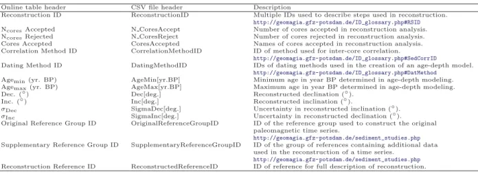
Online table header CSV file header Description
Reconstruction ID ReconstructionID Multiple IDs used to describe steps used in reconstruction.
http://geomagia.gfz-potsdam.de/ID_glossary.php#RSID
NcoresAccepted N CoresAccept Number of cores accepted in reconstruction analysis. NcoresRejected N CoresReject Number of cores rejected in reconstruction analysis. Cores Accepted CoresAccepted Names of cores accepted in reconstruction analysis. Correlation Method ID CorrelationMethodID ID of method used for inter-core correlation.
http://geomagia.gfz-potsdam.de/ID_glossary.php#SedCorrID
Dating Method ID DatingMethodID IDs of dating methods used in the creation of an age-depth model.
http://geomagia.gfz-potsdam.de/ID_glossary.php#DatMethod
Agemin(yr. BP) AgeMin[yr.BP] Minimum age in year BP determined in age-depth modeling. Agemax(yr. BP) AgeMax[yr.BP] Maximum age in year BP determined in age-depth modeling. Dec. (◦) Dec[deg.] Reconstructed declination (◦).
Inc. (◦) Inc[deg.] Reconstructed inclination (◦).
σDec SigmaDec[deg.] Uncertainty in reconstructed inclination (◦). σInc SigmaInc[deg.] Uncertainty in reconstructed declination (◦).
Original Reference Group ID OriginalReferenceGroupID ID of the reference group used to construct the original paleomagnetic time series.
http://geomagia.gfz-potsdam.de/sediment_studies.php
Supplementary Reference Group ID SupplementaryReferenceGroupID ID of the group of references containing additional data used in the reconstruction of a time series.
http://geomagia.gfz-potsdam.de/sediment_studies.php
Reconstruction Reference ID ReconstructedReferenceID ID of reference for full description of reconstruction.
Table S6: Field headers and descriptions unique to the ‘Reconstructed Paleomagnetic Time Series’ online table and