HAL Id: hal-00713669
https://hal-paris1.archives-ouvertes.fr/hal-00713669v2
Submitted on 2 Jul 2012HAL is a multi-disciplinary open access archive for the deposit and dissemination of sci-entific research documents, whether they are pub-lished or not. The documents may come from
L’archive ouverte pluridisciplinaire HAL, est destinée au dépôt et à la diffusion de documents scientifiques de niveau recherche, publiés ou non, émanant des établissements d’enseignement et de
Risk Aversion in the Euro area
Jonathan Benchimol
To cite this version:
Jonathan Benchimol. Risk Aversion in the Euro area. 29th GdRE Annual International Symposium on Money, Banking and Finance, Jun 2012, Nantes, France. �hal-00713669v2�
Risk aversion in the Euro area
Jonathan Benchimol February 14th, 2012
Abstract
We propose a New Keynesian Dynamic Stochastic General Equi-librium (DSGE) model where a risk aversion shock enters a separable utility function. We analyze …ve periods, each one lasting twenty years, to follow over time the dynamics of several parameters (such as the risk aversion parameter), the Taylor rule coe¢cients and the role of this risk aversion shock on output and real money balances in the Eurozone. Our analysis suggests that risk aversion was a more impor-tant component of output and real money balance dynamics between 2006 and 2011 than it had been between 1971 and 2006, at least in the short run.
Keywords: Risk aversion, Output, Money, Euro area, New Keyne-sian DSGE models, BayeKeyne-sian estimation.
JEL Classi…cation Number: E23, E31, E51.
Department of Economics, ESSEC Business School, Avenue Bernard Hirsch, 95021 Cergy Pontoise Cedex 2, France, and CES-University Paris 1 Panthéon-Sorbonne, 106-112 Boulevard de l’Hôpital, 75647 Paris cedex 13. Email: [email protected]. I would like to thanks Laurent Clerc (Banque de France), André Fourçans (ESSEC Business School), Marc-Alexandre Sénégas (Université Montesquieu Bordeaux IV) and an anony-mous referee for their useful comments.
1
Introduction
The New Keynesian model, as developed by Galí (2008) and Walsh (2010),
brings three equations together to characterize the dynamic behavior of three macroeconomic key variables: output, in‡ation, and the nominal interest rate. The resulting output equation corresponds to the log-linearization of an optimizing household’s Euler equation, linking consumption and output growth to the in‡ation-adjusted return on nominal bonds, that is, to the real interest rate. The in‡ation equation describes the optimizing behavior of monopolistically competitive …rms that either set prices in a randomly
staggered fashion, as suggested by Calvo (1983), or face explicit costs of
nominal price adjustment, as suggested by Rotemberg (1982). The nominal
interest rate equation, a monetary policy rule of the kind proposed byTaylor
(1993), dictates that the central bank should adjust the short-term nominal interest rate in response to a trade-o¤ between changes in in‡ation and output and changes in the past interest rate.
In this framework, even if money or real balances are included in the util-ity (MIU) or in the central bank’s reaction function, real or nominal monetary aggregates generally become an irrelevant variable and are then neglected, at
least for the US, as in Woodford (2003)andIreland (2004). Additionally, for
the Eurozone, even if a money variable appears in the monetary policy
reac-tion funcreac-tion, as inAndrés, López-Salido and Vallés (2006)or inBarthélemy,
Clerc, and Marx (2011), money plays no role in the dynamics.
However, Benchimol and Fourçans (2012) show that the role of money
in the business cycle is dependent on the risk aversion level, at least in the Eurozone. They estimate a New Keynesian DSGE model with non-separable
household preferences between consumption and money, as in the Ireland
(2004) or Andrés, López-Salido, and Nelson (2009) to analyze the role of money in the dynamics of the variables under a high level of risk aversion. In this context, they establish a signi…cant link between money, output and risk by showing that real money has a signi…cant role with regard to output and ‡exible-price output dynamics in the short term only if the relative risk aversion level is su¢ciently high (twice the standard value). They study the role of the level of risk aversion in a non-standard MIU function case and do not include a standard case or a study of a micro-founded risk aversion shock for the Eurozone. They only consider standard micro-founded shocks (price-markup, monetary policy and technology) and a money demand shock. Finally, as in other studies, we also consider a price-markup shock, a monetary policy shock and a technology shock. To analyze the role of risk aversion in the dynamics of other variables, we do not consider a money shock that has no role in the dynamics of this framework (because of the
separa-bility assumption between consumption and money), as shown bySmets and Wouters (2003), but we do consider a money equation to take account of the behaviors of national central banks (before 1999) and the European Central Bank (after 1999) and to close the model as much with historical variables as with exogenous shocks.
In contrast, as relative risk aversion measures the willingness to substi-tute consumption over di¤erent periods, the lower the level of risk aversion,
the more households substitute consumption over time. Wachter (2006)and
Bekaert, Engstrom, and Grenadier (2010) show that an increase in risk aver-sion involve an increase in equity and bond premiums and may increase the real interest rate through a consumption smoothing e¤ect or decrease it
through a precautionary savings e¤ect.Bommier, Chassagnon, and Le Grand
(2012) also show that risk aversion enhances precautionary savings. These studies con…rm the potential link between money holdings, output and risk aversion.
However, few studies quantify this link, or even consider risk aversion as a shock, in a New Keynesian DSGE framework. Moreover, no studies use
Bayesian techniques as Fernández-Villaverde (2010)does to analyze the role
of the risk aversion shock in output and money dynamics in the Eurozone. In
the nearly same technical and theoretical context, Alpanda (2012)highlights
the important role played by risk aversion shocks in US output between 2006 and 2011.
Accordingly, this article contributes to the literature in several ways. First, we analyze the role of a micro-founded risk aversion shock in the dynamics of a New Keynesian DSGE model. Second, the development of a completely micro-founded model with a risk aversion shock is original in terms of …ndings as well as in terms of estimation techniques. Mainly inspired by Smets and Wouters (2007) and Galí (2008), our model explores the role of risk aversion in in‡ation, output, interest rate and real money balances, as well as in ‡exible-price output..
A speci…c emphasis will be placed on how the risk aversion shock im-pacts the dynamics of these key variables through time. We use Bayesian
techniques, as in An and Schorfheide (2007), to estimate …ve subsamples of
the Eurozone between 1971 and 2011, each one lasting twenty years. This original focus on the last forty years will show that risk aversion shocks have had stronger e¤ects on output and real money balances in recent years than in the more distant past.
Last but not least, our framework allows us to analyze successively the informational content of the last two crises (subprimes and sovereign debts) in comparison with other crises that occurred between 1971 and 2006 in the Euro area.
Bayesian estimations and dynamic analyses of the model, with impulse response functions and short- and long-run variance decompositions following structural shocks, yield di¤erent relationships between risk aversion and other structural variables. This approach sheds light on the importance of risk aversion and its impact on output and real money balances during the last …ve years (2006 to 2011). It also shows that the role of monetary policy as regards output in the short run has decreased in the recent years in comparison to the more distant past.
Finally, this study explores with modern theoretical and empirical tools a fundamental question about the role of the perception of economic risks, e.g., the ability for households to consume now or later, in the dynamics of the main economic variables for the Eurozone.
Section 2 describes the theoretical set up. In Section 3, the model is
calibrated and estimated with Euro area data and impulse response func-tions and variance decomposition are analyzed. Interpretation of the results
is provided in Section 4. Section 5 concludes, and the Appendix presents
additional theoretical and empirical results.
2
The model
The model consists of households that supply labor, purchase goods for con-sumption and hold money and bonds, and of …rms that hire labor and pro-duce and sell di¤erentiated products in monopolistically competitive goods markets. Each …rm sets the price of the good it produces, but not all …rms reset their price during each period. Households and …rms behave optimally: households maximize the expected present value of utility, and …rms maxi-mize pro…ts. There is also a central bank that controls the nominal rate of
interest. This model is essentially inspired bySmets and Wouters (2007)and
Galí (2008).
2.1
Households
We assume a representative in…nitely lived household, seeking to maximize Et " 1 X k=0 kUt+k # (1)
where Ut is the period utility function and <1 is the discount factor. The
household decides how to allocate its consumption expenditures among the
for any given level of expenditures, as in Galí (2008). Furthermore, and conditional on such optimal behavior, the period budget constraint takes the form
PtCt+ Mt+ QtBt Bt 1+ WtNt+ Mt 1 (2)
where t = 0; 1; 2:::, Pt is an aggregate price index, Mt is the quantity of
money holdings at time t, Bt is the quantity of one-period nominally riskless
discount bonds purchased in period t and maturing in period t+1 (each bond
pays one unit of money at maturity and its price is Qt where it = log Qt
is the short term nominal rate), Wt is the nominal wage, and Nt is hours of
work (or the measure of household members employed). The above sequence
of period budget constraints is supplemented with a solvency condition1.
Preferences are measured with a common time-separable utility function (MIU). Under the assumption of a period utility given by
Ut = C 1 t t 1 t + 1 Mt Pt 1 Nt1+ 1 + (3)
consumption, money demand, labor supply, and bond holdings are chosen
to maximize (1) subject to (2) and the solvency condition. This MIU utility
function depends positively on the consumption of goods, Ct, positively on
real money balances, Mt
Pt, and negatively on labor Nt. t= + "
r
t is the
time-varying coe¢cient of the relative risk aversion of households (or the inverse
of the intertemporal elasticity of substitution), where "r
t is a risk aversion
shock. is the inverse of the elasticity of money holdings with respect to the
interest rate, and is the inverse of the elasticity of work e¤ort with respect
to the real wage. and are positive scale parameters.
This setting leads to the following conditions2, which, in addition to the
budget constraint, must hold in equilibrium. The resulting log-linear version of the …rst-order condition corresponding to the demand for contingent bonds implies that
ct= Et[ct+1]
1 t
(it Et[ t+1] c) (4)
where ct = ln (Ct) is the logarithm of the aggregate consumption, it is the
nominal interest rate, Et[ t+1] is the expected in‡ation rate in period t + 1
with knowledge of the information in period t, and c = ln ( ).
The demand for cash that follows from the household’s optimization prob-lem is given by
tct mpt m = a2it (5)
1Such as 8t lim n !1
Et[Bn] 0, in order to avoid Ponzi-type schemes.
where mpt = mt pt are the log linearized real money balances, m =
ln ( ) + a1, and a1 and a2 are resulting terms of the …rst-order Taylor
approximation of log (1 Qt) = a1+ a2it.
Real cash holdings depend positively on consumption with an elasticity
equal to t and negatively on the nominal interest rate3. In what follows, we
take the nominal interest rate as the central bank’s policy instrument. The resulting log-linear version of the …rst-order condition corresponding to the optimal consumption-leisure arbitrage implies that
wt pt= tct+ nt n (6)
where wt pt corresponds to the log of the real wage, nt denotes the log of
hours of work, and n = ln ( ).
Finally, these equations represent the Euler condition for the optimal
intratemporal allocation of consumption (Eq. (4)), the intertemporal
opti-mality condition setting the marginal rate of substitution between money
and consumption equal to the opportunity cost of holding money (Eq. (5)),
and the intratemporal optimality condition setting the marginal rate of
sub-stitution between leisure and consumption equal to the real wage (Eq. (6)).
2.2
Firms
Backus, Kehoe, and Kydland (1992)have shown that capital appears to play a rather minor role in the business cycle. To simplify the analysis and focus on the role of risk, we do not include a capital accumulation process in this
model, as in Galí (2008).
We assume a continuum of …rms indexed by i 2 [0; 1]. Each …rm produces a di¤erentiated good, but they all use an identical technology, represented by the following production function
Yt(i) = AtNt(i)1 (7)
where At = exp ("a
t) represents the level of technology, assumed to be
com-mon to all …rms and to evolve exogenously over time, and "a
t is a technology
shock.
All …rms face an identical isoelastic demand schedule and take the
ag-gregate price level Pt and aggregate consumption index Ct as given. As in
the standard Calvo (1983) model, our generalization features monopolistic
competition and staggered price setting. At any time t, only a fraction 1
of …rms, with 0 < <1, can reset their prices optimally, while the remaining
…rms index their prices to lagged in‡ation. 3Because 1 >1, a
2.3
Central bank
The central bank is assumed to set its nominal interest rate according to an
augmented smoothed Taylor (1993) rule such as:
it = (1 i) ( t c) + x yt ytf + m(mpt mpc) + iit 1+ "it
(8)
where , x and m are policy coe¢cients re‡ecting, respectively, the weight
on in‡ation, the output gap and real money; the parameter 0 < i < 1
captures the degree of interest rate smoothing; and "i
t is an exogenous ad
hoc shock accounting for ‡uctuations of the nominal interest rate. c is an
in‡ation target, and mpc is a money target, essentially included to account
for changes in targeting policies of in‡ation and monetary aggregates, as in,
respectively, Svensson (1999) and Fourçans and Vranceanu (2007)4.
m takes also into account the potential national central bank’s money
targeting before the creation of the European Central Bank (ECB, 1999). After 1999, the ECB follows an explicit money targeting until 2004 called
the Two Pillars policy, as explained inBarthélemy, Clerc, and Marx (2011),
and may even follow an implicit one after this date, as suggested by Kahn
and Benolkin (2007).
3
Empirical results
3.1
DSGE model
Our macro model consists of …ve equations and …ve dependent variables: in‡ation, nominal interest rate, output, real money balances, and ‡exible-price output. Flexible-‡exible-price output is completely determined by shocks.
yft = 1 + t(1 ) + + "at +(1 ) log (1 ) + n log " " 1 t(1 ) + + (9) t= Et[ t+1] + (1 ) (1 ) ( t(1 ) + + ) (1 + ") yt y f t (10) yt= Et[yt+1] t1(it Et[ t+1] c) (11) mpt= tyt a2it m (12)
4Other studies introduce a relevant money variable in the Euro area Taylor rule:
Andrés, López-Salido and Vallés (2006), Andrés, López-Salido, and Nelson (2009),
it = (1 i) ( t c) + x yt ytf + m(mpt mpc) + iit 1+ "it (13) where a1 = log 1 e 1 1 e1 1 and a2 = 1 e1 1.
All structural shocks are assumed to follow a …rst-order autoregressive
process with an i.i.d. normal error term, such as "k
t = k"kt 1+ !k;t, where
"k;t N(0; k) for k = fp; i; a; rg.
3.2
Euro area data
In our model of the Eurozone, t is the detrended in‡ation rate measured
as the yearly log di¤erence of the detrended GDP De‡ator from one quarter
to the same quarter of the previous year; yt is the detrended output per
capita measured as the di¤erence between the log of the real GDP per capita
and its trend; and itis the short-term (3-month) detrended nominal interest
rate. These data are extracted from the AWM database of Fagan, Henry,
and Mestre (2001). mpt is the detrended real money balances per capita measured as the di¤erence between the real money per capita and its trend, where real money per capita is measured as the log di¤erence between the money stock per capita and the GDP De‡ator. We use the M 3 monetary aggregate from the Eurostat database.
3.3
Calibration
Following standard conventions, we calibrate beta distributions for parame-ters that fall between zero and one, inverted gamma distributions for pa-rameters that need to be constrained to be greater than zero, and normal distributions in other cases.
The parameters of the utility function are assumed to be distributed as follows. Only the discount factor is …xed in the estimation procedure to 0:98. The intertemporal elasticity of substitution (i.e. the level of relative
risk aversion) is set at 2, a mean between the calibrations of Rabanal and
Rubio-Ramírez (2005)andCasares (2007), and consistent with the calibrated
value used by Kollmann (2001) and the value estimated by Lindé, Nessén,
and Söderström (2009). The inverse of the Frisch elasticity of labor supply is
assumed to be approximately 1, as in Galí (2008)and the scale parameters
on money and labor are assumed to be approximately 0:2, as in Benchimol
and Fourçans (2012).
The calibration of , , and " comes from Smets and Wouters (2007),
m) priors are calibrated followingSmets and Wouters (2003),Andrés, López-Salido, and Nelson (2009), and Barthélemy, Clerc, and Marx (2011). To observe both the behavior of the central bank and risk aversion, we assign a higher standard error (0:2) and a Normal prior law for the relative risk aversion level and for the Taylor rule’s coe¢cients (including the in‡ation and money targets), except for the smoothing parameter, which is restricted to
be positive and less than one (Beta distribution). The in‡ation target, c, is
calibrated to 2%, and the money target, mpc, is assumed to be approximately 4%.
The calibration of the shock persistence parameters and the standard
er-rors of the innovations followSmets and Wouters (2007). All of the standard
errors of shocks are assumed to be distributed according to inverted Gamma distributions, with prior means of 0:01. The latter ensures that these para-meters have positive support. The autoregressive parapara-meters are all assumed to follow Beta distributions. All of these distributions are centered approxi-mately 0:75, except for the autoregressive parameter of the monetary policy shock and the risk aversion shock, which are centered approximately 0:50, as in Smets and Wouters (2007). We take a common standard error of 0:15 for
the shock persistence parameters, which is a mean between that ofBenchimol
and Fourçans (2012) and Smets and Wouters (2007).
Law Mean Std. Law Mean Std.
beta 0.33 0.10 m normal 1.00 0.20 beta 0.66 0.10 c normal 2.00 0.20 normal 2.00 0.20 mpc normal 4.00 0.20 v normal 1.50 0.10 a beta 0.75 0.15 " normal 6.00 0.10 p beta 0.75 0.15 normal 1.00 0.10 i beta 0.50 0.15 beta 0.20 0.05 r beta 0.50 0.15 beta 0.20 0.05 a invgamma 0.01 2.00 i beta 0.50 0.10 p invgamma 0.01 2.00 normal 3.00 0.20 i invgamma 0.01 2.00 x normal 1.50 0.20 r invgamma 0.01 2.00
3.4
Results
The model is estimated with 160 observations from 1971 (Q1) to 2011 (Q1)
with Bayesian techniques, as in Smets and Wouters (2007). However, to
capture di¤erent policies and risk perceptions in the Euro area between 1971 and 2011, and more speci…cally between 2006 and 2011, we divide this large sample into …ve subsamples, each one consisting of 80 observations (20 years). This procedure allows us to analyze …ve di¤erent periods with a
su¢-ciently large sample, as speci…ed inFernandez-Villaverde and Rubio-Ramirez
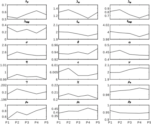
(2004). Accordingly, we estimate our model over …ve di¤erent periods: from 1971Q1 to 1991Q1 (P1); from 1976Q1 to 1996Q1 (P2); from 1981Q1 to 2001Q1 (P3); from 1986Q1 to 2006Q1 (P4); and from 1991Q1 to 2011Q1 (P5). 0.5 0.6 0.7 1.2 1.4 0.7 0.8 0.9 0 0.2 0.4 1.9 2 2.1 3.98 4 4.02 2.6 2.8 0.92 0.94 0.96 0.4 0.45 0.5 0.99 1 1.01 6 6.005 6.01 1.9 2 2.1 0.198 0.2 0.202 0.2 0.21 0.22 0.98 1 P1 P2 P3 P4 P5 0.6 0.8 1 P1 P2 P3 P4 P5 0.35 0.4 0.45 P1 P2 P3 P4 P5 0.9 0.95 1
Figure 1: Bayesian estimation of parameters over the selected periods The estimation of the implied posterior distribution of the parameters
over the …ve periods (Fig. 1) is performed using the Metropolis-Hastings
algorithm (10 distinct chains, each of 100000 draws). The average acceptation rates per chain are included in the interval [0:19; 0:22] and the student’s t-tests are all above 1:96. To assess the model validation, we insure convergence of the proposed distribution to the target distribution for each period in
Appendix6.B. Priors and posteriors distributions are presented in Appendix
6.C.
3.5
Simulations
3.5.1 Impulse response functions
As in the literature, Appendix 6.D (Fig. 9) shows that a price-markup
shock increases in‡ation and the nominal interest rate and decreases out-put, the output gap, the real interest rate, real money balances and real money growth.
The response of output, real money balances and real money growth to
a technology shock is positive (Fig. 9). Notice that the improvement in
technology is partly accommodated by the central bank, which lowers the nominal and real interest rate, while increasing the quantity of money in circulation.
Fig. 9 also presents the response to an interest rate shock. In‡ation,
output and the output gap, real money balances and real money growth all fall. The real and nominal interest rate rise.
This case is very interesting because Fig. 9 shows that a risk aversion
shock leads to a decrease in output and an increase in in‡ation: it implies a tightening of monetary policy (because of the strong weight that the central banker places on in‡ation), and its strength depends on the period (strong monetary policy tightening in P1 and low monetary policy tightening in P5). The risk aversion shock also implies an increase in real money balances and real money growth and a decrease in the output gap.
Household consumption is reduced (decreasing output), and companies increase their price (to face high risk aversion and possibly low consumption), which implies an increase in the in‡ation rate, constrained by a tightening of monetary policy.
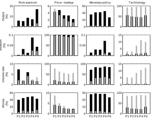
3.5.2 Variance decompositions
We analyze the forecast error variance decomposition of each variable follow-ing exogenous shocks. The analysis is conducted via an unconditional vari-ance decomposition to analyze long-term varivari-ance decomposition (the grey
bar in Fig. 2) and via a conditional variance decomposition, conditionally to
the …rst period, to analyze short-run variance decomposition (the black bar
in Fig. 2).
Fig. 2 shows that output is mainly explained by the technology shock
(ap-0 10 20 O ut pu t (%)
Ris k avers ion
0 2 4 6 Price- markup 0 20 40 60
Monetary pol icy
0 50 100 T echnology 0 0.05 0.1 Infl ati o n (%) 0 50 100 0 0.05 0.1 0 5 10 15 0 5 10 Inter es t rate (%) 0 50 100 0 50 100 0 5 10 15 P1 P2 P3 P4 P5 0 20 40 60 M o ney (%) P1 P2 P3 P4 P5 0 5 10 P1 P2 P3 P4 P5 0 10 20 30 P1 P2 P3 P4 P5 0 50 100
Figure 2: Long-term (grey) and short-term (black) variance decompositions proximately 35%) and the technology shock (approximately 50%) in the short run. The rest of the variance in output is explained by the risk aversion shock (approximately 5% from P1 to P4 and more than 15% for P5) in the short term, whereas risk aversion shock has a limited role in output variance in the long run.
Fig. 2 also shows that, in accordance with the literature, in‡ation is
mainly explained by the price-markup shock and that interest rate variance is mainly driven by monetary policy in the short run and by monetary policy and price-markup in the long run. Furthermore, most of the variance in real money balances is induced by the risk aversion shock (approximately 40%) and the monetary policy shock (approximately 25%) in the short run, whereas in the long run, real money balance variance is mainly driven by the technology shock. All of these results are in line with the literature.
4
Interpretation
Appendix 6.B shows that the estimation results are valid and that
that the maximum of the posterior distribution reaches the posterior mean of each estimated parameter. The estimation is relatively well identi…ed, and the data are quite informative for most of the estimated micro-parameters.
Fig. 9shows that from P1 to P5, the impact of the price-markup shock
on in‡ation and output is almost halved. It also shows that the risk aversion shock has a longer impact in P5 than it does in the other periods. This is due to the increase over the periods of the autoregressive parameter of the
risk aversion shock, r, as shown in Fig. 1.
Fig. 2 shows that output and real money balances variances have an
important component coming from the risk aversion shock. This …nding shows the leading role of relative risk aversion in the dynamics of output,
as in Black and Dowd (2011), and of real money balances, as in Benchimol
and Fourçans (2012). Although the in‡ation rate, the nominal interest rate and the ‡exible-price output are strong components of output, risk aversion has a minor role to play in the variance of in‡ation and interest rate, and it has also no role to play with regard to the ‡exible-price output (less than 0:2% in the short and long run), which is completely determined by the technology shock. It also shows that in‡ation and interest rate variances are quasi una¤ected by the introduction of the risk aversion shock, letting these variables be mainly explained by, respectively, the price-markup shock and the monetary policy shock.
The leading role of the risk aversion shock in the dynamics of real money
balances in the short run is another important …nding. Fig. 2shows that real
money balances are mainly explained by the technology shock (approximately 80%) in the long run, whereas in the short run, real money balances are mainly explained by the risk aversion shock and the monetary policy shock.
Fig. 2shows that technology plays an increasingly important role in the
short term for the in‡ation rate and, thus, the interest rate through the selected periods. This …gure also shows that, in the short run, risk aversion has a more signi…cant role in output dynamics in the last period (P5) than in the other periods (P1 to P4). This …nding re‡ects the increasing role assumed by risk aversion in more recent years (between 2006 and 2011) as compared to the past (between 1971 and 2006).
Finally, Fig. 2 shows that monetary policy has a lower role in the short
run concerning output in the last period (P5), approximately 22%, than it had in the past, approximately 35%. It highlights the transfer from the monetary policy role to the risk aversion role during the recent years. This con…rms the declining in‡uence of European monetary policy relative to the in‡uence of risk aversion shocks.
5
Conclusion
Risk aversion is a concept in economics and …nance that is based on the behavior of consumers and investors who are exposed to uncertainty. It is the reluctance of a person to accept a bargain with an uncertain payo¤ rather than another bargain o¤ering a more certain, but possibly lower, expected payo¤.
This paper presents a standard New Keynesian DSGE model that includes a risk aversion shock. It shows the involvement of this risk aversion shock in
the dynamics of the economy: it increases in‡ation, decreases output (Fig. 9)
and diminishes the impact of the central bank’s actions on output variance,
at least in the short run (Fig. 2). Risk aversion plays also an important role
for output and real money balance dynamics. The negative role played by risk aversion in determining output is clearly identi…ed, whereas it increases
real money balances and real money growth in the …rst periods (Fig. 9).
Moreover, while estimations are quite robust (Fig. 3 to Fig. 8), they
show that the risk aversion shock has a stronger impact on output dynamics during the last twenty years (P5) as compared to other analyzed periods (P1 to P4). This result is explained by the inclusion in P5 of the subprime and sovereign debt crises from 2007 to 2011.
This enhanced baseline model shows the importance of such a parameter to the economy, and especially its impact on output, money, and monetary policy. It also serves to show how it is important to control shocks to the risk aversion of agents, by communication for example.
6
Appendix
A
Solving the model
Price dynamics
Let’s assume a set of …rms not reoptimizing their posted prices in period t. Using the de…nition of the aggregate price level and the fact that all …rms
re-setting prices choose an identical price Pt, leads to Pt=h P1 t
t 1 + (1 ) (Pt) 1 ti 1 1 t , where t = 1 + 1 1 " 1+" p
t is the elasticity of substitution between consumption
goods in period t, and t
t 1 is the markup of prices over marginal costs (time
varying). Dividing both sides by Pt 1 and log-linearizing around Pt = Pt 1
yields
In this setup, we do not assume inertial dynamics of prices. In‡ation results from the fact that …rms reoptimizing in any given period their price plans, choose a price that di¤ers from the economy’s average price in the previous period.
Price setting
A …rm reoptimizing in period t chooses the price Pt that maximizes
the current market value of the pro…ts generated while that price remains e¤ective. This problem is solved and leads to a …rst-order Taylor expansion around the zero in‡ation steady state:
pt pt 1 = (1 )
1 X k=0
( )kEt mct+kjtc + (pt+k pt 1) (15)
wheremct+kjtc = mct+kjt mcdenotes the log deviation of marginal cost from
its steady state value mc = , and = log "
" 1 is the log of the desired gross markup.
Equilibrium
Market clearing in the goods market requires Yt(i) = Ct(i) for all i 2 [0; 1]
and all t. Aggregate output is de…ned as Yt = R01Yt(i)1 1t di
t
t 1
; it
follows that Yt = Ct must hold for all t. One can combine the above goods
market clearing condition with the consumer’s Euler equation (4) to yield
the equilibrium condition
yt= Et[yt+1] t1(it Et[ t+1] c) (16)
Market clearing in the labor market requires Nt=R01Nt(i) di. With the
production function (7) and taking logs, one can write the following
approx-imate relationship between aggregate output, employment and technology as
yt= "a
t + (1 ) nt (17)
An expression is derived for an individual …rm’s marginal cost in terms of the economy’s average real marginal cost:
mct = (wt pt) mpnt (18)
= wt pt 1
1 ("
a
for all t, where mpntde…nes the economy’s average marginal product of labor.
As mct+kjt= (wt+k pt+k) mpnt+kjt we have
mct+kjt = mct+k t
1 (pt pt+k) (19)
where the second equality follows from the demand schedule combined with
the market clearing condition ct= yt. Substituting (19) into (15) yields
pt pt 1 = (1 ) 1 X k=0 t+k( )kEt[mct+kc ] + 1 X k=0 ( )kEt[ t+k] (20)
where t = 1 1+ t 1 is time varying to take into account the markup
shock.
Finally, (14) and (20) yield the in‡ation equation
t= Et[ t+1] + mctmctc (21)
where , mct =
(1 )(1 )
t. mct is strictly decreasing in the index of
price stickiness , in the measure of decreasing returns , and in the demand
elasticity t.
Next, a relationship is derived between the economy’s real marginal cost
and a measure of aggregate economic activity. From (6) and (17), the average
real marginal cost can be expressed as
mct = t+ + 1 yt 1 + 1 " a t log (1 ) n (22)
Under ‡exible prices, the real marginal cost is constant and equal to mc =
. De…ning the natural level of output, denoted by yft, as the equilibrium
level of output under ‡exible prices leads to
mc= t+ + 1 y f t 1 + 1 " a t log (1 ) n (23) thus implying ytf = a"at + c (24) where a = t(1 1+)+ + and c = (1 )(log(1 )+ n log(""1)) t(1 )+ + . Subtracting (25) from (24) yields c mct= t+ + 1 yt y f t (25)
wheremctc = mct mcis the real marginal cost gap and yt yft is the output
gap. Combining the above equation with (23), we obtain
t= Et[ t+1] + x yt y f t (26) where x = (1 )(1 )( t(1 )+ + ) (1 + ") and yt y f
t is the output gap.
The second key equation describing the equilibrium of the model is
ob-tained by rewriting (19) to determine output
yt= Et[yt+1] t1(it Et[ t+1] c) (27)
Equation (27) is thus a dynamic IS equation including the real money
balances.
The third key equation describes the behavior of the real money balances.
From (5), we obtain mpt= t yt a2 it m (28)
B
Model validation
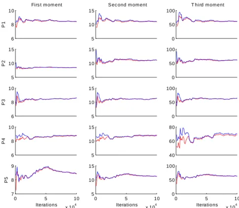
The red and blue lines in Fig. 3represent an aggregate measure based on the
eigenvalues of the variance-covariance matrix of each parameter both within and between chains. Each graph represents speci…c convergence measures and has two distinct lines that represent the results within and between chains. Those measures are related to the analysis of the parameter’s mean (…rst moment), variance (second moment) and third moment of the model in the considered period. Convergence requires that both lines for each of the three measures become relatively constant and converge to each other.
The diagnoses concerning the numerical maximization of the posterior kernel indicate that the optimization procedure was able to obtain a robust maximum for the posterior kernel. A diagnosis of the overall convergence for
the Metropolis-Hastings sampling algorithm is provided in Fig. 3.
Diagnoses for each individual parameter were also obtained, following the same structure as that of the overall. Most of the parameters do not seem to exhibit convergence problems, notwithstanding the fact that this evidence is stronger for some parameters than it is for others.
6 8 10
P1
Firs t mom ent
5 10 15 S ec ond m oment 0 50 100 T hi rd moment 5 10 15 P2 5 10 15 0 50 100 6 8 10 P3 5 10 15 0 50 100 6 8 10 P4 5 10 15 40 60 80 0 5 10 x 104 7 8 9 Iterations P5 0 5 10 x 104 5 10 15 Iterations 0 5 10 x 104 0 50 100 Iterations
Figure 3: Multivariate Metropolis-Hastings convergence diagnosis
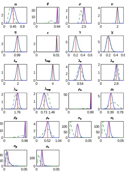
C
Priors and posteriors
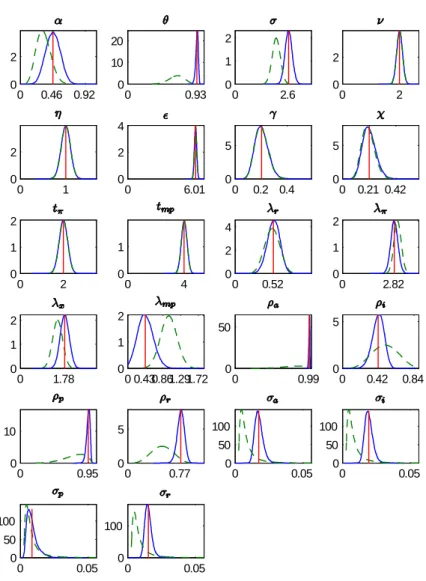
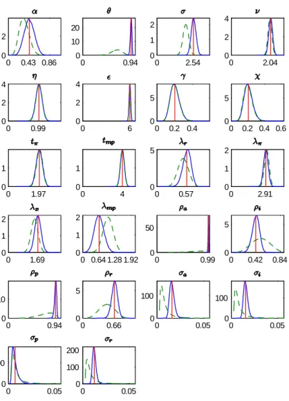
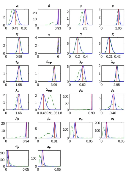
The vertical red line denotes the posterior mode, the dashed green line the prior distribution, and the blue line the posterior distribution.
0 0.45 0.9 0 2 0 0.94 0 10 20 0 2.5 0 1 2 0 2 0 2 4 0 0.99 0 2 0 6.01 0 2 0 0.2 0.4 0.6 0 5 0 0.2 0.4 0.6 0 5 0 2 0 1 0 4 0 1 0 0.54 0 2 4 0 2.8 0 1 2 0 1.76 0 1 2 0 0.73 1.46 0 1 2 0 0.99 0 50 0 0.39 0.78 0 5 0 0.96 0 10 20 0 0.52 1.04 0 2 4 0 0.05 0 50 100 0 0.05 0 50 100 0 0.05 0 50 100 0 0.05 0 100
0 0.46 0.92 0 2 0 0.93 0 10 20 0 2.6 0 1 2 0 2 0 2 0 1 0 2 0 6.01 0 2 4 0 0.2 0.4 0 5 0 0.21 0.42 0 5 0 2 0 1 2 0 4 0 1 0 0.52 0 2 4 0 2.82 0 1 2 0 1.78 0 1 2 0 0.430.861.291.72 0 1 2 0 0.99 0 50 0 0.42 0.84 0 5 0 0.95 0 10 0 0.77 0 5 0 0.05 0 50 100 0 0.05 0 50 100 0 0.05 0 50 100 0 0.05 0 100
0 0.43 0.86 0 2 0 0.94 0 10 20 0 2.54 0 1 2 0 2.04 0 2 4 0 0.99 0 2 4 0 6 0 2 4 0 0.2 0.4 0 5 0 0.2 0.4 0.6 0 5 0 1.97 0 1 0 4 0 1 0 0.57 0 5 0 2.91 0 1 2 0 1.69 0 1 2 0 0.64 1.28 1.92 0 1 2 0 0.99 0 50 0 0.42 0.84 0 5 0 0.94 0 10 0 0.66 0 5 0 0.05 0 100 0 0.05 0 100 0 0.05 0 100 0 0.05 0 100 200
0 0.43 0.86 0 2 0 0.93 0 10 20 0 2.5 0 1 2 0 2.06 0 2 4 0 0.99 0 2 0 6 0 2 4 0 0.2 0.4 0 5 0 0.21 0.42 0 5 0 1.95 0 1 0 3.99 0 1 0 0.62 0 5 0 2.95 0 1 2 0 1.66 0 1 2 0 0.450.91.351.8 0 1 2 0 0.99 0 50 100 0 0.46 0 5 0 0.94 0 10 20 0 0.81 0 5 0 0.05 0 100 0 0.05 0 100 200 0 0.05 0 100 200 0 0.05 0 100
0 0.43 0.86 0 2 0 0.95 0 20 0 2.51 0 1 2 0 2.05 0 2 4 0 0.99 0 2 0 6 0 2 0 0.2 0.4 0.6 0 5 0 0.2 0.4 0 5 0 1.98 0 1 0 4 0 1 0 0.56 0 5 0 2.95 0 1 2 0 1.66 0 1 2 0 0.73 1.46 0 1 2 0 0.99 0 50 0 0.42 0.84 0 5 0 0.95 0 10 20 0 0.9 0 10 0 0.05 0 100 0 0.05 0 100 200 0 0.05 0 100 0 0.05 0 100 200
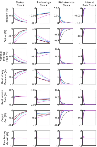
D
Impulse response functions
The black line, blue line, red line, cyan line and magenta line, represent, respectively the P5, P4, P3, P2 and P1 impulse response functions.
0 0.5 1 Markup Shock Infl ati o n ( % ) - 0.4 - 0.2 0 O u tp ut ( % ) 0 0.5 1 N o m inal Inter es t R at e (% ) - 1 - 0.5 0 R e al M on ey B a la n ce s (% ) - 0.2 0 0.2 R ea l Int er e st R at e (% ) - 0.4 - 0.2 0 O ut pu t G a p ( %) - 1 0 1 R e al M on ey G rowt h ( % ) - 0.1 - 0.05 0 T echnology Shock 0.5 1 1.5 - 0.2 - 0.1 0 0.5 1 1.5 - 0.05 0 0.05 - 1 - 0.5 0 - 2 0 2 0 0.01 0.02 Risk Aversion Shock - 0.4 - 0.2 0 0 0.2 0.4 0 1 2 0 0.2 0.4 - 0.4 - 0.2 0 - 2 0 2 - 0.01 - 0.005 0 Interest Rate Shock - 1 - 0.5 0 0 0.5 1 - 2 - 1 0 0 0.5 1 - 1 - 0.5 0 - 2 0 2
References
Adolfson, M., 2007. Bayesian estimation of an open economy DSGE model with incomplete pass-through. Journal of International Economics 72(2), 481-511.
Alpanda, S., 2012. Identifying the Role of Risk Shocks in the Business Cycle Using Stock Price Data. Economic Inquiry, forthecoming.
An, S., and Schorfheide, F., 2007. Bayesian Analysis of DSGE Models. Econo-metric Reviews 26(2-4), 113-172.
Andrés, J., López-Salido, D.J., and Nelson, E., 2009. Money and the natural rate of interest: Structural estimates for the United States and the euro area. Journal of Economic Dynamics and Control 33(3), 758-776. Andrés, J., López-Salido, J.D., Vallés, J., 2006. Money in an Estimated
Busi-ness Cycle Model of the Euro Area. Economic Journal 116(511), 457-477. Backus, D.K., Kehoe, P.J., and Kydland, F.E., 1992. International Real
Busi-ness Cycles. Journal of Political Economy 100(4), 745-75.
Barthélemy, J., Clerc, L., and Marx, M., 2011. A two-pillar DSGE monetary policy model for the euro area. Economic Modelling 28(3), 1303-1316. Black, D., Dowd, M., 2011. Risk aversion as a technology factor in the
pro-duction function. Applied Financial Economics 21(18), 1345-1354. Bekaert, G., Engstrom, E., and Grenadier, S.R., 2010. Stock and bond
re-turns with Moody Investors. Journal of Empirical Finance 17(5), 867-894.
Benchimol, J., and Fourçans, A., 2012. Money and risk in a DSGE framework: A Bayesian application to the Eurozone. Journal of Macroeconomics, forthcoming.
Bommier, A., Chassagnon, A., and Le Grand, F., 2012. Comparative Risk Aversion: A Formal Approach with Applications to Saving Behaviors. Journal of Economic Theory, forthcoming.
Calvo, G.A., 1983. Staggered prices in a utility-maximizing framework. Jour-nal of Monetary Economics 12(3), 383-398.
Casares, M., 2007. Monetary Policy Rules in a New Keynesian Euro Area Model. Journal of Money, Credit and Banking 39(4), 875-900.
Fagan, G., Henry, J., and Mestre, R., 2001. An area-wide model (AWM) for the Euro area. European Central Bank Working Paper No. 42.
Fernández-Villaverde, J., 2010. The econometrics of DSGE models. SERIEs 1(1), 3-49.
Fernandez-Villaverde, J., and Rubio-Ramirez, J.F., 2004. Comparing dy-namic equilibrium models to data: a Bayesian approach. Journal of Econometrics 123(1), 153-187.
Fourcans, A., and Vranceanu, R., 2007. The ECB monetary policy: Choices and challenges. Journal of Policy Modeling 29(2), 181-194.
Galí, J., 2008. Monetary Policy, In‡ation and the Business Cycle: An Intro-duction to the New Keynesian Framework. Princeton University Press. Ireland, P.N., 2004. Money’s role in the monetary business cycle. Journal of
Money, Credit and Banking 36(6), 969-983.
Kahn, G.A., and Benolkin, S., 2007. The role of money in monetary pol-icy: why do the Fed and ECB see it so di¤erently ?. Economic Review, Federal Reserve Bank of Kansas City Q3, 5-36.
Kollmann, R., 2001. The exchange rate in a dynamic-optimizing business cycle model with nominal rigidities: a quantitative investigation. Journal of International Economics 55(2), 243–262.
Lindé, J., Nessén, M., and Söderström, U., 2009. Monetary policy in an esti-mated open-economy model with imperfect pass-through. International Journal of Finance and Economics 14(4), pages 301-333.
Rabanal, P., and Rubio-Ramirez, J.F., 2005. Comparing New Keynesian models of the business cycle: A Bayesian approach. Journal of Monetary Economics 52(6), 1151-1166.
Rotemberg, J., 1982. Monopolistic Price Adjustment and Aggregate Output. Review of Economic Studies 49(4), 517-31.
Smets, F.R., and Wouters, R., 2003. An Estimated Dynamic Stochastic Gen-eral Equilibrium Model of the Euro Area. Journal of the European Eco-nomic Association 1(5), 1123-1175.
Smets, F.R., and Wouters, R., 2007. Shocks and frictions in US business cycles: a Bayesian DSGE approach. American Economic Review 97(3), 586-606.
Svensson, L.E.O., 1999. In‡ation targeting as a monetary policy rule. Journal of Monetary Economics 43(3), 607-654.
Taylor, J.B., 1993. Discretion versus Policy Rules in Practice. Carnegie-Rochester Conference Series on Public Policy 39, 195-214.
Wachter, J.A., 2006. A consumption-based model of the term structure of interest rates. Journal of Financial Economics 79(2), 365-399.
Walsh, C.E., 2010. Monetary theory and policy. Cambridge, MA.: The MIT Press.
Woodford, M., 2003. Foundations of a Theory of Monetary Policy. Princeton University Press.