Behavioral uncertainty and the dynamics of traders' confidence in their price forecasts

(1)

HAL Id: hal-01712301

https://hal.archives-ouvertes.fr/hal-01712301

Submitted on 19 Feb 2018

HAL is a multi-disciplinary open access

archive for the deposit and dissemination of

sci-entific research documents, whether they are

pub-lished or not. The documents may come from

teaching and research institutions in France or

abroad, or from public or private research centers.

L’archive ouverte pluridisciplinaire HAL, est

destinée au dépôt et à la diffusion de documents

scientifiques de niveau recherche, publiés ou non,

émanant des établissements d’enseignement et de

recherche français ou étrangers, des laboratoires

publics ou privés.

Behavioral uncertainty and the dynamics of traders’

confidence in their price forecasts

Nobuyuki Hanaki, Eizo Akiyama, Ryuichiro Ishikawa

To cite this version:

Nobuyuki Hanaki, Eizo Akiyama, Ryuichiro Ishikawa. Behavioral uncertainty and the dynamics of

traders’ confidence in their price forecasts. Journal of Economic Dynamics and Control, Elsevier,

2018, 88, pp.121 - 136. �10.1016/j.jedc.2018.01.020�. �hal-01712301�

(2)

Behavioral uncertainty and the dynamics of traders’

confidence in their price forecasts

∗

Nobuyuki Hanaki

†

Eizo Akiyama

‡

Ryuichiro Ishikawa

§

January 8, 2018

Abstract

By how much does the presence of behavioral uncertainty in an experimental asset market reduce subjects’ confidence in their price forecasts? An incentivized interval forecast elicitation method is employed to answer this question. Each market consists of six traders, and the value of dividends is known. Two treatments are considered: six human traders (6H), and one human interacting with five computer traders whose behavior is known (1H5C). We find that while the deviation of the initial price forecasts from fundamental value is smaller in the 1H5C treatment than in the 6H treatment, albeit not statistically significantly, the average confidence regarding the forecasts is not. We further analyze the relationships between subjects’ confidence in their forecasts and their trading behavior, as well as their trading performance, in the 6H treatment. While subjects’ high confidence in their short-term forecasts shows a negative correlation with their trading performance, high confidence in their long-term forecasts shows a positive correlation with trading performance.

Keywords: Price forecasts, interval elicitation, experimental asset markets, behavioral uncertainty JEL Code: C90, D84

∗_{Makoto Soga provided invaluable help in organizing the experiments. This project is partly financed by L’Institute}

Universitaire de France, by JSPS KAKENHI Grant Numbers 26285043, 26350415, 26245026, 26590026, and 17K18569, by ANR ORA-Plus project “BEAM” (ANR-15-ORAR-0004), by a grant-in-aid from the Zengin Foundation for Stud-ies on Economics and Finance, and by the French government-managed l’Agence Nationale de la Recherche under Investissements d’Avenir U CAJ EDI _{(ANR-15-IDEX-01). In particular, we thank the UCAinACTION project. We}

thank Geoff Whyte from Edanz Group (www.edanzediting.com/ac) for proof-reading a draft of this manuscript. The authors declare no conflicts of interest associated with this manuscript. The experiments reported in this paper have been approved by the Institutional Review Board of the Faculty of Engineering, Information and Systems, University of Tsukuba (No. 2012R25-1).

†_Universit´_{e Cˆ}_{ote d’Azur, CNRS, GREDEG, France. Corresponding author. GREDEG, 250 rue Albert Einstein,}

06560 Valbonne, FRANCE. E-mail: [email protected]

‡_{Faculty of Engineering, Information and Systems, University of Tsukuba. E-mail: [email protected]} §_{School of International Liberal Studies, Waseda University. E-mail: [email protected]}

(3)

1 Introduction

By how much does the presence of behavioral uncertainty reduce subjects’ confidence in their price forecasts? We aim to answer this question by employing an interval forecast elicitation method (Schlag and van der Weele, 2013) using the framework of Akiyama et al. (2017), who examine the effect of uncertainty about other traders’ behavior (behavioral uncertainty) on the initial deviation of price forecasts from fundamental value (FV) in an experimental asset market a la Smith et al. (1988).

The interval forecast elicitation method allows us to measure the confidence subjects have in each of their forecasts by asking subjects to submit ranges (between 0% and 19% in our study) around their forecasts within which they believe future prices will fall. The process is incentivized in that the narrower the range submitted, the higher the reward when the future prices fall within the range specified.

As Palan (2013) notes, despite the large body of literature employing the experimental framework of Smith et al. (1988), there is only a limited number of studies investigating the dynamics of forecasts (Haruvy et al., 2007; Akiyama et al., 2014, 2017; Bosch-Rosa et al., 2017; Eckel and F¨ullbrunn, 2015) or the relationship between the dynamics of forecasts, trading behavior, and market outcomes (Carle et al., 2017) despite the fact that the possibility of directly eliciting price forecasts from market participants is one of the great advantages of laboratory experiments.

Furthermore, existing studies investigating forecast dynamics do not measure the degree of con-fidence market participants place in their price forecasts. We believe that measuring the degree of confidence will add additional insights because, as Scheinkman and Xiong (2003) show theoretically, heterogeneity among subjects regarding their confidence in their ability to forecast future prices can be an important source of speculative bubbles that are accompanied by large trading volumes and high price volatility. Odean (1998) also demonstrates theoretically that overconfident traders trade more and obtain lower expected payoffs than they would if they were not overconfident.

Such theoretical predictions are supported by Biais et al. (2005), Deaves et al. (2009), and Michailova and Schmidt (2016), who study the relationship between subjects’ degree of “overcon-fidence” (or “miscalibration,” to be more precise), their performance, and the degree of mispricing observed in the markets. These studies measure subjects’ degree of “overconfidence” based on a psychological test that asks subjects to answer multiple questions by providing an interval in

(4)

re-sponse to each question such that they are 90% sure that the correct answer will fall within the interval (Russo and Schowmaker, 1991), and then correlate their performance with (or in the case of Michailova and Schmidt (2016), construct a market based on) the measured degree of miscalibration. However, these studies do not directly measure the confidence subjects have in their price forecasts within asset markets.

To the best of our knowledge, one exception is Kirchler and Maciejovsky (2002). Their study measures the degree of subjects’ confidence in their price forecasts by eliciting, at the beginning of each period, (a) an interval (defined by high and low forecasts) within which subjects believe the current period price will fall with 98% likelihood, and (b) their subjective degree of confidence regarding the accuracy of their forecasts (on a nine-point scale ranging from not certain to certain). The results show that subjects tend to do poorly in calibrating their forecast intervals (the realized prices are outside the stated interval in more than 30% of cases), and their subjective degree of confidence tends to perform well in capturing the accuracy of their forecasts. However, it should be noted that subjects were not provided with any monetary incentive in relation to their forecasting performance.

Our study takes an additional step forward in that our interval forecast elicitation method is incentivized so that subjects who are more confident in the accuracy of their forecasts will submit narrower forecast ranges. We elicit, at the beginning of each period, both forecasts and their ranges for all the remaining periods, which allows us to observe the dynamics of forecasts, confidence levels, trading behavior, and market outcomes. As the first step toward such a rich set of analyses, we investigate how much subjects’ confidence in their forecasts is affected by the presence of behavioral uncertainty, as well as how it evolves in two clearly distinct realizations of price dynamics.

We have chosen to study the effect of behavioral uncertainty on subjects’ confidence to comple-ment recent studies on the causes of mispricing observed in expericomple-mental asset markets a al Smith et al. (1988). Bosch-Rosa et al. (2017) suggest that the mispricing is mainly due to the low cognitive ability of market participants, while Hanaki et al. (2017a) suggest that not only the average cognitive ability of market participants but also their heterogeneity matters in determining the magnitude of the mispricing. Kirchler et al. (2012) and Huber and Kirchler (2012) suggest that the mispricing is mainly due to subjects’ misunderstanding of the declining nature of FV, while Cheung et al. (2014) suggest that even if the subjects themselves understand the declining nature of FV, their uncertainty about others’ understanding of the nature of FV can generate significant mispricing. Along a

(5)

simi-lar line, Akiyama et al. (2017) show that the presence of uncertainty about other traders’ behavior results in greater mispricing in subjects’ forecasts. An obvious question that follows from the result of Akiyama et al. (2017) is whether the presence of behavioral uncertainty also influences subjects’ confidence in their forecasts.

Our results show that while eliminating behavioral uncertainty makes the initial forecasts of our subjects closer, albeit not statistically significantly, to the FV of the asset, it does not increase our subjects’ confidence in their initial forecasts. It is only after subjects have observed prices following a deterministic path for a few periods that their confidence in their price forecasts begins to increase. Further, we analyze the relationships between subjects’ confidence in their forecasts, trading behavior, and trading performance. We find that when subjects have a high level of confidence in their forecasts, at least in the first round in which they participate, they tend to increase their bids more when they expect a greater price increase in future periods. We also find that while trading performance is negatively correlated with subjects’ confidence in their short-term forecasts, it is positively correlated with their confidence in their long-term forecasts.

The rest of the paper is organized as follows. Section 2 describes the experimental design, the results are presented in Section 3, and Section 4 concludes.

2 Experiment

We consider asset market experiments a la Smith et al. (1988) with interval forecast elicitation (Schlag and van der Weele, 2013). Below, we explain the market environment, the interval forecast elicitation method we use, and the two treatments we consider.

2.1 Markets

In both of the treatments, a group of six traders trade an asset with a life of 10 periods. All of the traders receive four units of the asset and 520 experimental currency units (ECUs) as their initial endowment. Each unit of the asset pays a dividend of 12 ECUs at the end of each period. After the final dividend payment in period 10, the asset loses its value. Therefore, the FV of the asset at the beginning of period t, F Vt, is 12(11 − t) ECUs. Note that we have eliminated the

uncertainty associated with dividend payments in each period because we are interested in the effect of uncertainty about others’ behavior on traders’ confidence in their forecasts.

(6)

We employ a call market structure for trading among subjects as in van Boening et al. (1993), Haruvy et al. (2007), Akiyama et al. (2014, 2017), and Bosch-Rosa et al. (2017). In call markets, unlike in continuous double auctions, there is one market clearing price for the asset in each period. Having only one price per period is advantageous for experiments with future price forecasts because the future prices to be forecasted are defined very clearly.1

In our call market experiment, subjects can submit a buy order and a sell order in each period by separately specifying a price and quantity for each type of order. If subject i decides to submit a buy order in period t, he must specify the maximum price at which he is willing to buy a unit of the asset (bi

t, for bid) and the maximum number of units that he is willing to buy (dit) in that

period. Similarly, to submit a sell order in period t, a subject must specify the minimum price at which he is willing to sell a unit of the asset (ai_t, for ask) and the maximum number of units he is willing to sell (si_t) in that period. Of course, subjects can decide to submit neither a buy order nor a sell order by setting the quantities in both types of order to zero. We impose three constraints on the orders subjects can submit: the admissible price range, a budget constraint, and the relationship between bi

t and ait in the case where a subject submits both buy and sell orders.

The admissible price range is set such that when di

t≥ 1 (sit≥ 1), bit(ait) must be an integer between

1 and 2000, i.e., bi

t ∈ {1, 2, ..., 2000} (ait ∈ {1, 2, ..., 2000}). The budget constraint simply means

that neither borrowing of cash nor short-selling is allowed.2 _{The final constraint means that when}

a trader submits both buy and sell orders, the ask price must be no less than the bid price, ai t≥ bit.

We imposed a 60-second, non-binding time limit for submission of orders. When the time limit was reached, the subjects were told, via a message flashing in the upper right corner of their screen, to submit their orders as soon as possible.

Once all of the traders in the market have submitted their orders, the price that clears the market is calculated3 _{and all transactions are processed at that price among traders who submitted a bid}

no less than, or an ask no greater than, the market clearing price.4

1_{Our experimental setup is based on that of Akiyama et al. (2014, 2017).} 2_{Thus, the budget constraint implies (i) d}i

t× bit ≤ cash holding at the beginning of the period, and (ii) sit ≤

units of the asset on hand at the beginning of the period.

3_{Following the design of Haruvy et al. (2007), when there are several such prices, the lowest price is chosen as the}

market clearing price. This is important because it ensures that the price does not spike upward in the absence of transactions at the market clearing price.

4_{Any ties among the last accepted buy or sell orders are resolved randomly. It is possible that no transactions take}

(7)

2.2 Interval forecast elicitation

In addition to trading units of an asset in a call market, at the beginning of each period (i.e., prior to submitting their orders), subjects are asked to submit price forecasts for each of the remaining periods, as well as the ranges ({0%, 1%, ..., 19%}) within which they think the market prices will fall.

That is, in period t, subject i submits 11 − t forecasts, fi

t,k, for period k prices, pk, k ∈ {t, ..., 10},

and 11 − t corresponding ranges, wi

t,k ∈ {0, 1, ..., 19} (in percentage terms) around their forecasts.

Subjects obtained bonus points of (20 − wi_t,k), when pk was

pk ∈ [(1 − wt,ki /100)ft,ki , (1 + wit,k/100)ft,ki ]. (1)

As can easily be seen, wider forecast ranges were penalized in that they generated lower bonus points.

The bonus points for all 55 price forecasts over the 10 periods were summed.5 _{Let B}i_{be the total}

number of points subject i obtained over 10 periods. Subjects were rewarded for their forecasting performance with a bonus payment in addition to what they obtained from their trading performance as follows:

Bonus (in ECUs) = 0.05% × Bi× cash holding after period 10. (2)

For example, if wi

t,k = 0 for all t and k, and the realized prices in all 10 periods were equal to

the forecast prices fi

t,k for all t and k, the subject received 20 × 55 = 1100 points. As a result, the

subject received an additional 55% of his cash holding at the end of period 10 as a bonus.6

5_{Because subjects are making 11-t forecasts at the beginning of period t, they make a total of 55 forecasts during}

the 10 periods.

6_{Note that paying subjects for both forecasting and trading performances as we do in this paper may cause subjects}

to hedge between the two activities, as discussed by Bao et al. (2013). This issue is studied by Hanaki et al. (2017b) (but without eliciting forecast ranges as we do in the current study), who investigate whether eliciting price forecasts and the way in which subjects are rewarded for their forecast performance influence the market outcomes in the framework of Smith et al. (1988). They report that eliciting price forecasts and rewarding subjects based on both their forecasting and trading performance (for example, in the form of bonus payments as we do here) generates significantly higher mispricing than in experiments without forecast elicitation or with forecast elicitation but where subjects are paid based on either their forecasting or trading performance, but not on both. In the latter case, the selection between the trading and the forecasting performances on which subjects’ payment is based is done randomly at the end of the experiment. Hanaki et al. (2017b) also report, however, that the way in which subjects are rewarded for their forecasting performance (e.g., either in addition to their trading performance or instead of their trading performance) does not significantly affect their forecasting performance. Thus, it is possible that the mispricing observed in our experiment is affected by the way in which we reward subjects based on their forecasting performance, but that its effect on forecasting performance may be limited. The effect of the incentive scheme we used (i.e., a bonus payment for forecasting performance in addition to a reward for trading performance) on the forecast

(8)

We imposed a 20 × (11 − t)-second, non-binding time limit for submission of price forecasts in period t. When the time limit was reached, the subjects were told, via a message flashing in the upper right corner of their screen, to submit their forecasts as soon as possible.

2.3 Treatments

We consider two treatments: one in which all six traders in a market are humans, and another in which only one of the six traders in a market is a human and the remaining five are computerized traders. We call the former treatment 6H and the latter treatment 1H5C.

All of the computerized traders in the 1H5C treatment behave in the following manner. In each period, they submit both buy and sell orders under the budget constraint restriction by setting bt= at= F Vt.

Subjects are told which treatment they are in. That is, those in the 6H treatment are told that all of the other five traders in their market are subjects participating in the same experiment, while those in the 1H5C treatment are told that all of the other five traders in their market are computer programs. The behavior of the computerized traders is explained to subjects in the 1H5C treatment, but not to those in the 6H treatment, as follows. After explaining how to submit orders, the way the market price in each period is determined based on the submitted orders, and the dividend process (and the meaning of “Next Value”, the term we use for FV in each period), subjects in the 1H5C treatment are told that “In each period, each computer trader submits orders by setting both the maximum price it is willing to pay and the minimum price it is willing to accept for a stock equal to the Next Value at the beginning of that period.”7 _{Thus, subjects in the 1H5C treatment do not}

face any uncertainty regarding the behavior of other traders in the market, while those in the 6H treatment do.

Akiyama et al. (2017) employ the same framework, comparing the forecasts elicited in the 6H and 1H5C treatments, except that they do not elicit the forecast ranges. The reward for accurate forecasting (fi

t,k) is computed based on the number of forecasts (out of the 55 that a subject submits)

that are within 10% of the realized price, that is, subjects receive a bonus equivalent to 0.5% of their final cash holding if their forecast price for period k, pk, is 0.9pk ≤ ft,ki ≤ 1.1pk.8

range is not known.

7_{An English translation of the instructions is provided in the Appendix B.}

8_{Furthermore, in Akiyama et al. (2017), subjects had 120 seconds instead of the 20 × (11 − t)-second, non-binding}

(9)

Table 1: Number of subjects and markets in the two treatments. Number of subjects Number of markets

6H 72 12

1H5C 61 61

Akiyama et al. (2017) found that the 10 initial forecasts submitted by subjects participating in the 1H5C treatment deviated significantly less from FV than those submitted by subjects in the 6H treatment, suggesting that the presence of behavioral uncertainty has a significant effect on subjects’ expectations of market prices. They also found that while the observed differences in the deviations of the initial forecasts from FV between the two treatments were significantly positive for those subjects who scored highly in the cognitive reflection test (CRT, Frederick, 2005), this was not the case for those with very low CRT scores (0 or 1).

To complement the finding of Akiyama et al. (2017), we are interested in comparing the confidence our subjects have in their forecasts (measured by wi

t,k) in the two treatments. All subjects repeated

the experiment in the same group of traders with the same initial endowment and the same dividend payments, i.e., subjects participated in two rounds of 10 periods each. They were paid the sum of their final cash holding from trading and receipt of dividends, as well as bonuses from the two rounds in which they participated.

3 Results

The experiments were conducted at the University of Tsukuba between January and July 2016.9 A total of 133 subjects, 72 in the 6H treatment and 61 in the 1H5C treatment, participated in the experiment. These subjects had never participated in similar experiments, and they participated exclusively in one of the two treatments. Table 1 summarizes the number of subjects participating as well as the number of markets (six subjects per market in the 6H treatment and one subject per market in the 1H5C treatment) in the two treatments.

Below, we first investigate the effect of behavioral uncertainty on subjects’ initial price forecasts and on their confidence in the forecasts by comparing the results of the 6H and 1H5C treatments. Next, we demonstrate the dynamics of realized prices in the 6H and 1H5C markets, subjects’ price forecasts, and their confidence in their forecasts. Finally, we focus on the subjects’ confidence in

(10)

RAF Di,m₁ wi,m₁ 0.0 0.5 1.0 1.5 2.0 2.5 3.0RAFD 0.0 0.2 0.4 0.6 0.8 1.0 CDF 0 5 10 15 20<w> 0.0 0.2 0.4 0.6 0.8 1.0 CDF p = 0.567 p = 0.521

Figure 1: Cumulative distribution of RAF D1 (left) and w1 (right) in the 6H (solid red line) and

1H5C (dashed blue line) treatments in period 1 of Round 1. P-values are from the two-sample permutation test (two-tailed).

their short-term and long-term forecasts in the 6H treatment and analyze the relationships between subjects’ short-term/long-term confidence, their trading orders, and their trading performance.

3.1 Initial forecasts and their deviations from FV

We follow Akiyama et al. (2017) in measuring the magnitude of the deviations of forecasts submit-ted by subject i in market m in period t from FV using the relative absolute forecast deviation (RAF Di,m_t ), which is defined as:

RAFDi,m_t = 1 T − t + 1 T X k=t |f_t,ki,m− F Vk| |F V | , (3)

where f_t,ki,mis the forecast asset price in period k submitted by subject i in market m at the beginning of period t.10

We also consider the average forecast range submitted by subject i in market m in period t, wi,m_t :

wi,m_t = PT k=tw i,m t,k T − t + 1 . (4)

Figure 1 shows the cumulative distribution of the initial forecast deviations, RAF Di,m₁ , (left) and the initial average forecast range, wi,m₁ , (right) in Round 1 for the 6H (solid red line) and 1H5C (dashed blue line) treatments. Based on the findings of Akiyama et al. (2017), we expect RAF D₁i,m 10_{For clarity of exposition, we omit super/subscripts indicating the round. In the exposition below, we show the}

(11)

in the 1H5C treatment to be smaller than that in the 6H treatment. We also expect that, given that subjects are informed about the behavior of the five computer traders in the market, wi,m₁ in the 1H5C treatment will be smaller than that in the 6H treatment, that is, subjects in the former treatment will be more confident in their forecasts than those in the latter.

As expected, the distribution of RAF Di,m₁ for the 1H5C treatment, shown in the left panel of Figure 1, lies to the left of that for the 6H treatment. The difference is, however, not statistically significant even at the 10% level according to the two-tailed two-sample permutation test (p = 0.567). Thus, we fail to replicate the main finding of Akiyama et al. (2017). This failure in replication may be due to (a) the additional complications introduced by the interval forecast elicitation method, (b) a shorter time limit for entering forecasts (although the limit is not binding), or (c) a smaller sample size for the 1H5C treatment in our experiment than that of Akiyama et al. (2017).11

Contrary to our expectations, our data show that the distribution of the average forecast range wi,m₁ in the 1H5C and 6H treatments mirror each other (p = 0.521, two-sample permutation test, two-tailed). Subjects in the 1H5C treatment, while forecasting prices closer to FV than those in the 6H treatment, are initially no more confident in their forecasts than subjects in the 6H treatment. Thus, we need to investigate the dynamics of forecasts and their ranges to observe the treatment effects.12

3.2 Dynamics of forecast deviations and confidence

It is useful to review the price dynamics before discussing the forecast dynamics because exist-ing studies demonstrate that forecasts tend to be adaptive (see, for example, Haruvy et al., 2007; Akiyama et al., 2014).

11_{Furthermore, Akiyama et al. (2017) use the Mann–Whitney test, which has lower power than the permutation}

test we use in this study. Applying the Mann–Whitney test (two-tailed) to our data, we find that p=0.138, which is still not significant at the 10% level, but closer to the result of Akiyama et al. (2017).

12_{Eckel and F¨}_{ullbrunn (2015) and Cueva and Rustichini (2015) investigate the effect of gender composition on}

market outcomes. They find that all-female markets result in smaller mispricing than all-male markets. This is often understood to be the result of gender differences in terms of risk preferences (females tend to be more risk-averse than males) and competitiveness (males tend to be more competitive than females). It is also possible that this result is due to gender differences in terms of degree of overconfidence. Barber and Odean (2001), for example, find that males tend to be more (over)confident than females. We found a statistically significant gender difference in terms of wi,m₁ in the 1H5C treatment, but not in the 6H treatment. There were 43 male and 18 female subjects in the 1H5C treatment and 59 male and 13 female subjects in the 6H treatment. In the 1H5C treatment, the average wi,m1 was

8.61 for males and 10.54 for females (p=0.025, two-sample permutation test, two-tailed). In the 6H treatment, the corresponding figures were 9.44 for males and 9.89 for females (p=0.617). Furthermore, we found that RAF Di,m₁ was significantly higher for female subjects in both treatments. The average RAF Di,m₁ was 1.03 and 3.56 for male and female subjects, respectively, in the 6H treatment (p=0.019), and 0.66 and 2.45, respectively, in the 1H5C treatment (p=0.022).

(12)

6H. Round 1 6H. Round 2 1 2 3 4 5 6 7 8 9 10t 50 100 150 200 250 P 1 2 3 4 5 6 7 8 9 10t 50 100 150 200 250 P 1H5C. Round 1 1H5C. Round 2 1 2 3 4 5 6 7 8 9 10t 50 100 150 200 250 P 1 2 3 4 5 6 7 8 9 10t 50 100 150 200 250 P

Figure 2: Price dynamics over two rounds in the 6H treatment (top) and 1H5C treatment (bottom).

Figure 2 shows the dynamics of realized prices in Round 1 (left) and Round 2 (right) in the 6H treatment (top) and 1H5C treatment (bottom). Not surprisingly, given the way our computer traders behave, the prices in the 1H5C treatment follow FV, while the prices in the 6H treatment deviate from FV, with smaller deviations in Round 2 than in Round 1. We are interested in investigating how this difference in the price dynamics between the two treatments influences the dynamics of forecasts and confidence.

Figures 3 and 4 show, for two groups from the 6H treatment, the dynamics of price forecasts (with the error bars representing the forecast ranges computed based on the submitted forecast range in % terms) and the forecast ranges (in % terms) elicited at the beginning of each period over the two rounds. Figures 3 shows the outcomes of a group where prices did not follow FV, while Figure 4 shows the outcomes where prices followed FV.

In both groups, the initial sets of price forecasts elicited at the beginning of period 1 of Round 1 vary substantially among subjects.13 _{The confidence levels (in terms of the elicited forecast ranges)}

also vary across subjects. Once subjects observe the realized price in period 1 (of Round 1), however, the forecasts for the period 2 price that are elicited at the beginning of period 2 become quite similar

(13)

6H, Group 9, Round 1 6H, Group 9, Round 2 Forecasts Ranges Forecasts Ranges

t=1 t=1 t=1 t=1 1 2 3 4 5 6 7 8 9 10t 0 50 100 150 200 250 300P 1 2 3 4 5 6 7 8 910t 0 5 10 15 20w 1 2 3 4 5 6 7 8 9 10t 0 50 100 150 200 250 300P 1 2 3 4 5 6 7 8 910t 0 5 10 15 20w t=2 t=2 t=2 t=2 1 2 3 4 5 6 7 8 9 10t 0 50 100 150 200 250 300P 1 2 3 4 5 6 7 8 910t 0 5 10 15 20w 1 2 3 4 5 6 7 8 9 10t 0 50 100 150 200 250 300P 1 2 3 4 5 6 7 8 910t 0 5 10 15 20w t=3 t=3 t=3 t=3 1 2 3 4 5 6 7 8 9 10t 0 50 100 150 200 250 300P 1 2 3 4 5 6 7 8 910t 0 5 10 15 20w 1 2 3 4 5 6 7 8 9 10t 0 50 100 150 200 250 300P 1 2 3 4 5 6 7 8 910t 0 5 10 15 20w t=4 t=4 t=4 t=4 1 2 3 4 5 6 7 8 9 10t 0 50 100 150 200 250 300P 1 2 3 4 5 6 7 8 910t 0 5 10 15 20w 1 2 3 4 5 6 7 8 9 10t 0 50 100 150 200 250 300P 1 2 3 4 5 6 7 8 910t 0 5 10 15 20w t=5 t=5 t=5 t=5 1 2 3 4 5 6 7 8 9 10t 0 50 100 150 200 250 300P 1 2 3 4 5 6 7 8 910t 0 5 10 15 20w 1 2 3 4 5 6 7 8 9 10t 0 50 100 150 200 250 300P 1 2 3 4 5 6 7 8 910t 0 5 10 15 20w t=6 t=6 t=6 t=6 1 2 3 4 5 6 7 8 9 10t 0 50 100 150 200 250 300P 1 2 3 4 5 6 7 8 910t 0 5 10 15 20w 1 2 3 4 5 6 7 8 9 10t 0 50 100 150 200 250 300P 1 2 3 4 5 6 7 8 910t 0 5 10 15 20w t=7 t=7 t=7 t=7 1 2 3 4 5 6 7 8 9 10t 0 50 100 150 200 250 300P 1 2 3 4 5 6 7 8 910t 0 5 10 15 20w 1 2 3 4 5 6 7 8 9 10t 0 50 100 150 200 250 300P 1 2 3 4 5 6 7 8 910t 0 5 10 15 20w t=8 t=8 t=8 t=8 1 2 3 4 5 6 7 8 9 10t 0 50 100 150 200 250 300P 1 2 3 4 5 6 7 8 910t 0 5 10 15 20w 1 2 3 4 5 6 7 8 9 10t 0 50 100 150 200 250 300P 1 2 3 4 5 6 7 8 910t 0 5 10 15 20w t=9 t=9 t=9 t=9 1 2 3 4 5 6 7 8 9 10t 0 50 100 150 200 250 300P 1 2 3 4 5 6 7 8 910t 0 5 10 15 20w 1 2 3 4 5 6 7 8 9 10t 0 50 100 150 200 250 300P 1 2 3 4 5 6 7 8 910t 0 5 10 15 20w t=10 t=10 t=10 t=10 1 2 3 4 5 6 7 8 9 10t 0 50 100 150 200 250 300P 1 2 3 4 5 6 7 8 910t 0 5 10 15 20w 1 2 3 4 5 6 7 8 9 10t 0 50 100 150 200 250 300P 1 2 3 4 5 6 7 8 910t 0 5 10 15 20w

(14)

6H, Group 12, Round 1 6H, Group 12, Round 2 Forecasts Ranges Forecasts Ranges

(15)

1H5C, subjects 1-6, Round 1 1H5C, subjects 1-6, Round 2 Forecasts Ranges Forecasts Ranges

(16)

among the six subjects in the market. Meanwhile, the long-term forecasts (those for period 3 and beyond) elicited in period 2 continue to vary among subjects. This convergence of short-term forecasts (those for the current period price) across subjects and the persistence of heterogeneity in the long-run forecasts (those for the prices in the remaining future periods) is observed throughout Round 1 in both Figure 3 and 4. It is interesting to note that there is no clearly observable pattern in the change in the dynamics of forecast ranges between two consecutive periods in Round 1.14

In Round 2, the initial sets of forecasts submitted in period 1 are very similar among subjects in the same group, and they closely resemble the dynamics of prices observed over 10 periods in Round 1. Conversely, the initial sets of forecast ranges in Round 2 continue to vary among subjects, remaining at 10% on average, just as in Round 1. Thus, we can infer that while the prices observed in the previous round are acting as anchors for the forecasts in Round 2, just as the price observed in the previous period acted as an anchor for the current short-run forecast in Round 1, they do not necessarily increase subjects’ confidence in their price forecasts. Furthermore, although the dynamics of realized prices follows a similar path to that observed in Round 1 in the groups shown in Figures 3 and 4 during the first few periods in Round 2, there is no clear decline in the elicited forecast ranges (in % terms).

This is in sharp contrast with the observed dynamics of the forecasts and forecast ranges for the six subjects in the 1H5C treatment shown in Figure 5. As in the case of subjects in the 6H treatment, the initial set of forecasts and forecast ranges elicited at the beginning of period 1 of Round 1 vary among subjects. Once the realized price is observed, the short-run forecasts converge toward the observed price, while the heterogeneity in the long-run forecasts persists for the first couple of periods. By period 3 of Round 1, however, four of the six subjects plotted in Figure 5 learn the implications of the behavior of the five computers in the market and start to forecast prices that follow FV with high degrees of confidence (i.e., small forecast ranges). At the beginning of Round 2, most of the subjects forecast prices to follow FV over 10 periods, and three of the six subjects do so with certainty (i.e., confidence ranges of 0% for all periods).

The difference in the dynamics of confidence between the 6H and 1H5C treatments (especially when prices follow FV quite closely in the 6H treatment) suggests that the confidence level increases 14_{In Appendix A, we report that the changes in the confidence levels for short-term forecasts between two consecutive}

periods are not related to the magnitudes of forecasting errors in the previous period in the 6H treatment. We also report, for the same treatment, that when subjects have a high level of confidence in their forecasts for future periods, they adjust their forecasts significantly less given the magnitude of their forecasting errors in the previous period.

(17)

when subjects figure out the reason for the price dynamics they observe. In the 1H5C treatment, prices following FV can be linked very easily to the known behavior of the computer traders, which is known to remain the same. In the 6H treatment, even though the prices follow FV quite closely, subjects cannot be sure that prices will continue to do so in the future because they are unsure about the future behavior of other traders.

The outcomes shown in Figures 3 to 5 characterize the basic differences in the dynamics of forecasts and confidence between the 6H and 1H5C treatments. To see this clearly, we present an aggregate analysis below. Because the six subjects in the same market are observing the same realized prices before updating their price forecasts in the 6H treatment, their forecasts are not independent. For the analyses below, we take an average of RAF Di,m_t , as well as wi,m_t , across traders within a market to compute the average RAF Dm_t and wm_t for price forecasts and ranges submitted by traders in period t in market m. Below, we use this within-market average (across subjects in a market) as an independent observation.

Figure 6 shows the dynamics of the median RAF Dm

t (top) and wmt (bottom) for the 6H (solid red

line) and 1H5C (dashed blue line) treatments over two rounds. As noted above, the median RAF Dm

is smaller in the 1H5C treatment than in the 6H treatment in period 1 of Round 1, although the difference is not statistically significant. We also observe that the median RAF Dm_{s declines rapidly}

in both the 1H5C and 6H treatments in the first couple of periods in Round 1. The median RAF Dm

in the 1H5C treatment becomes zero by period 5 of Round 1 and remains there until the end of Round 2. The median RAF Dm _{in the 6H treatment remains positive, except for the last couple}

of periods in Round 2, reflecting the deviations from FV of the observed prices in the 6H markets. The differences in RAF Dm between the two treatments are, however, not statistically significant according to the two-tailed two-sample permutation test in any period.

The median wm _{in period 1 of Round 1 is almost 10 in both the 6H and 1H5C treatments. In}

the 1H5C treatment, wm_{only begins to decline after period 3 and remains positive until period 10,}

despite the fact that subjects in the 1H5C treatment observe prices mirroring FV in every period and quickly adjust their forecasts to be closer to FV. At the beginning of Round 2, the median wm becomes positive again in the 1H5C treatment and takes a few periods to return to zero, although the median RAF D continues to be zero from the beginning of Round 2. Conversely, for the 6H treatment, the median wm only declines slightly over the two rounds, although the decline in wm during Round 2 is more pronounced than that during Round 1.

(18)

Median RAF Dm t Round 1 Round 2 1 2 3 4 5 6 7 8 9 10t 0.5 1.0 1.5 2.0 RAFD 1 2 3 4 5 6 7 8 9 10t 0.0 0.5 1.0 1.5 2.0 RAFD

P-values from two sample permutation test (two-tailed)

Period 1 2 3 4 5 6 7 8 9 10 Round 1 0.642 0.583 0.810 0.622 0.332 0.330 0.329 0.329 0.326 0.328 Round 2 0.113 0.331 0.331 0.331 0.330 0.326 0.329 0.329 0.327 0.328 Median wm_t Round 1 Round 2 1 2 3 4 5 6 7 8 9 10t 0 5 10 15 20<w> 1 2 3 4 5 6 7 8 9 10t 0 5 10 15 20<w>

P-values from two sample permutation test (two-tailed)

Period 1 2 3 4 5 6 7 8 9 10

Round 1 0.717 0.832 0.499 0.178 0.041 0.003 0.003 0.003 0.0001 0.0004 Round 2 0.0001 0.0003 0.0006 0.0001 0.0002 0.0001 0.00003 0.0005 0.0002 0.0003 Figure 6: Dynamics of the median RAF Dm

t (top) and wmt (bottom) in the 6H (solid red line) and

1H5C (dashed blue line) treatments over two rounds. P-values from the two-sample permutation test (two-tailed) are reported.

3.3 Analyses of 6H treatment

Below, we provide further analyses of the relationships between subjects’ confidence in their forecasts, trading behavior, and trading performance for the 6H treatment. In particular, we focus on the effects of subjects’ confidence on their short-term and long-term forecasts.

Carle et al. (2017) report, based on their analyses of the data from Haruvy et al. (2007), that short-term forecasts (i.e., forecasts of the current period price) are better determinants of trading behavior than long-term forecasts (i.e., the average of forecasts for all remaining periods).15 That 15_{More precisely, Carle et al. (2017) characterize long-term forecasts as the average deviation of forecasts from FV.}

(19)

is, they find that while short-term forecasts have a statistically significant relationship with trading behavior, long-term forecasts do not. Our aim here is to determine how subjects’ confidence in their short-term and long-term forecasts relates to their trading behavior.

Carle et al. (2017) characterize subjects’ long-term forecasts based on their average relative deviation from FV. However, this fails to capture the types of price paths that subjects are expecting. For example, subjects may expect prices to remain constant in the future, or to rise initially and then fall. Such differences in dynamics will be hidden if the average of these future forecasts is used. Thus, in our analyses, we characterize them differently by focusing on the first peak or the first valley that appears in subjects’ long-term forecasts.

Let us consider a series of forecasts that subject i (in market m) submits at the beginning of period t. We define subject i’s maximum long-term forecast in period t, hi,m_t , and its timing, τ hi,m_t , as well as subject i’s long-term minimum forecast in period t, li,mt , and its timing, τ l

i,m t , as follows: hi,mt = max k>t f i,m t,k (5)

τ hi,m_t = min argmax

k>t f_t,ki,m (6) li,m_t = min k>tf i,m t,k (7)

τ li,m_t = min argmin

k>t

f_t,ki,m. (8)

As can be seen, we consider the maximum and minimum forecasts that are closest to period t in defining τ hi,m_t and τ li,m_t . We then consider the following five types of forecast paths:

(1) Peak then valley: if l_ti,m< f_t,ti,m< hi,m_t and τ hi,m_t < τ li,m_t

(2) Valley then peak: if lti,m< f i,m t,t < h i,m t and τ l i,m t < τ h i,m t

(3) Up: if f_t,ti,m ≤ li,mt < h i,m t

(4) Down: if li,m_t < hi,m_t ≤ ft,ti,m

(5) Flat: if li,m_t = hi,m_t = f_t,ti,m.

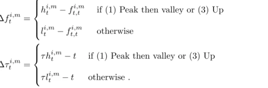
Finally, we define the price increase (or decrease) that subject i expects between period t and the price peak (or valley), ∆f_ti,m, and the number of periods before the peak (or valley), ∆τ_ti,m,

(20)

depending on the type of forecast path as follows: ∆f_ti,m =       

hi,m_t − f_t,ti,m if (1) Peak then valley or (3) Up li,m_t − f_t,ti,m otherwise

(9) ∆τti,m =       

τ hi,m_t − t if (1) Peak then valley or (3) Up τ l_ti,m− t otherwise .

(10)

We also compute the mean confidence of subject i in his forecasts between period t and the peak (or valley) as:

b w_ti,m= P∆τti,m k=t+1w i,m t,k ∆τti,m . (11)

To facilitate our interpretation, we define two dummy variables, HCS_ti,m (for short-term fore-casts) and HCLi,mt (for long-term forecasts), that capture whether subject i’s confidence in his

short-term and long-term forecasts in period t is high. More specifically, HCSi,mt takes a value of

1 if w_t,ti,m ≤ K and HCLi,mt takes a value of 1 ifwb

i,m

t ≤ K. We consider two values of K, K = 5

(Def 1) and K = 7 (Def 2). These two values represent the 33rd and 50th percentiles, respectively, of wi,m_t across all periods in both rounds for all of the subjects in the 6H treatment. Note that according to these definitions of the HCS and HCL dummies, a subject’s confidence in a given period can be high in relation to his short-term forecasts but low regarding his long-term forecasts (and vice versa). It is also possible that his confidence in his forecasts (short term and/or long term) can be high in some periods and low in other periods.

Equipped with these measures, we first analyze the relationship between subjects’ confidence in their forecasts and trading behavior, and then investigate the relationship with trading performance.

3.3.1 Forecasts, confidence, and trading behavior

We are interested in how subject i’s bid, bi

t, and ask, ait, in period t depend on his short-term

forecasts, f_t,ti,m, and associated level of confidence, HCS_ti,m, as well as his long-term forecasts and the associated levels of confidence that are summarized by ∆f_ti,m, ∆τ_ti,m, and HCLi,m_t . We also investigate the interactions between the levels of confidence and the forecasts.

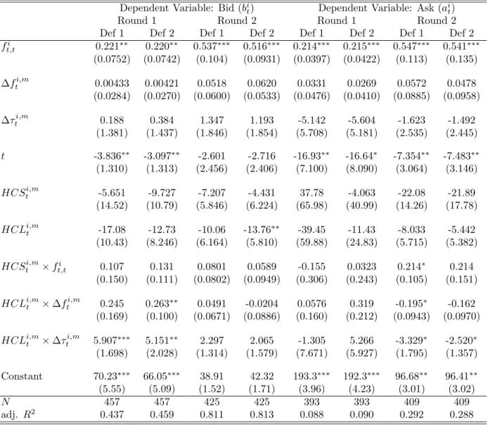
Table 2 shows the results of subject fixed-effect regressions. The standard errors are corrected for the within-group clustering effect. Eight regression results are reported in Table 2: four for bids,

(21)

Table 2: Effects of forecasts and levels of confidence on bids, bi

t, and asks, ait .

Dependent Variable: Bid (bi

t) Dependent Variable: Ask (ait)

Round 1 Round 2 Round 1 Round 2 Def 1 Def 2 Def 1 Def 2 Def 1 Def 2 Def 1 Def 2 fi t,t 0.221∗∗ 0.220∗∗ 0.537∗∗∗ 0.516∗∗∗ 0.214∗∗∗ 0.215∗∗∗ 0.547∗∗∗ 0.541∗∗∗ (0.0752) (0.0742) (0.104) (0.0931) (0.0397) (0.0422) (0.113) (0.135) ∆fti,m 0.00433 0.00421 0.0518 0.0620 0.0331 0.0269 0.0572 0.0478 (0.0284) (0.0270) (0.0600) (0.0533) (0.0476) (0.0410) (0.0885) (0.0958) ∆τ_ti,m 0.188 0.384 1.347 1.193 -5.142 -5.604 -1.623 -1.492 (1.381) (1.437) (1.846) (1.854) (5.708) (5.181) (2.535) (2.445) t -3.836∗∗ -3.097∗∗ -2.601 -2.716 -16.93∗∗ -16.64∗ -7.354∗∗ -7.483∗∗ (1.310) (1.313) (2.456) (2.406) (7.100) (8.090) (3.064) (3.146) HCSi,m_t -5.651 -9.727 -7.207 -4.431 37.78 -4.063 -22.08 -21.89 (14.52) (10.79) (5.846) (6.224) (65.98) (40.99) (14.26) (17.78) HCLi,m_t -17.08 -12.73 -10.06 -13.76∗∗ _-39.45 _-11.43 _-8.033 _-5.442 (10.43) (8.246) (6.164) (5.810) (59.88) (24.83) (5.715) (5.382) HCSi,m_t × fi t,t 0.107 0.131 0.0801 0.0589 -0.155 0.0323 0.214∗ 0.214 (0.150) (0.111) (0.0802) (0.0949) (0.306) (0.243) (0.105) (0.151) HCLi,mt × ∆f i,m t 0.245 0.263∗∗ 0.0491 -0.0204 0.0576 0.319 -0.195∗ -0.162 (0.169) (0.100) (0.0671) (0.0886) (0.160) (0.212) (0.0943) (0.0970) HCLi,m_t × ∆τ_ti,m 5.907∗∗∗ 5.151∗∗ 2.297 2.065 -1.305 5.266 -3.329∗ -2.520∗ (1.698) (2.028) (1.314) (1.579) (7.671) (5.927) (1.795) (1.357) Constant 70.23∗∗∗ 66.05∗∗∗ 38.91 42.32 193.3∗∗∗ 192.3∗∗∗ 96.68∗∗ 96.41∗∗ (5.55) (5.09) (1.52) (1.71) (3.96) (4.23) (3.01) (3.02) N 457 457 425 425 393 393 409 409 adj. R2 _0.437 _0.459 _0.811 _0.813 _0.088 _0.090 _0.292 _0.288

Robust standard errors corrected for the within-group clustering effect are shown in parentheses.

(22)

bi,m_t , and four for asks, ai,m_t . There are four regressions for bids and four for asks because we have two definitions of high-confidence dummies and two rounds.

First, we note that the measures we use capture the variations in bids better than those in asks, as confirmed by the higher R2 in bid regressions than in ask regressions.16 Second, we note that while the short-run forecasts, f_t,ti,m, have a positive and statistically significant effect on both bids and asks, neither of our two measures of long-run forecasts, ∆f_ti,m and ∆τ_ti,m, has a statistically significant effect. We also note, as one would expect based on the declining FV, that the estimated coefficient of time trend t is negative and statistically significant in both bid and ask regressions, except for bid regressions in Round 2.

Our two dummy variables for a high level of confidence in short-term and long-term forecasts, HCSi,m_t and HCLi,m_t , have negative but statistically insignificant estimated coefficients except for HCLi,mt for bid regressions under definition 2 in Round 2. However, it is interesting to note that the

estimated coefficients for the interaction terms between HCLi,mt and ∆f i,m

t , as well as ∆τ i,m t , in the

bid regressions in Round 1 are positive and statistically significant, especially under definition 2. This suggests that, at least in Round 1, when subjects’ confidence regarding their long-term forecasts is high, their bids respond more positively to the expected changes in prices and the duration between the future peak (or valley) and the current period than when their confidence in their long-term forecasts is low.

3.3.2 Confidence in forecasts and trading performance

How does the relationship between subjects’ confidence in their price forecasts and their trading behavior manifest in terms of their trading performance? We investigate this question using summary statistics of subjects’ confidence in their short-term and long-term forecasts over 10 periods.

We define subject i’s degree of confidence in his short-term and long-term forecasts over 10 periods in a market, with an abuse of notations HCSi,m _{and HCL}i,m_{, respectively, based on the}

dummy variables we defined above as follows:

HCSi,m=X t HCSti,m (12) HCLi,m=X t HCLi,m_t . (13)

(23)

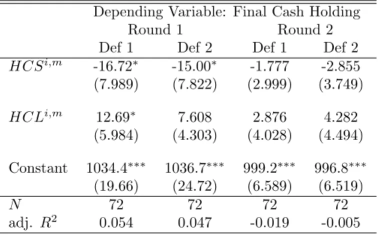
Table 3: Confidence in forecasts and trading performance. Depending Variable: Final Cash Holding

Round 1 Round 2 Def 1 Def 2 Def 1 Def 2 HCSi,m _-16.72∗ _-15.00∗ _-1.777 _-2.855 (7.989) (7.822) (2.999) (3.749) HCLi,m _12.69∗ _7.608 _2.876 _4.282 (5.984) (4.303) (4.028) (4.494) Constant 1034.4∗∗∗ 1036.7∗∗∗ 999.2∗∗∗ 996.8∗∗∗ (19.66) (24.72) (6.589) (6.519) N 72 72 72 72 adj. R2 _0.054 _0.047 _-0.019 _-0.005

∗_{p < 0.10,}∗∗ _{p < 0.05,}∗∗∗ _{p < 0.01}

Here, we are interested in whether subjects who tend to be highly confident in their forecasts over 10 periods perform better in terms of their final cash holding than other subjects. Because we are interested in trading performance, we do not include the bonus for forecasting performance in our performance measure.

Table 3 reports the results of ordinary least squares regressions. The dependent variable is the cash holding at the end of period 10. As above, we consider two definitions of high-confidence dummies for short-term and long-term forecasts. The results show that in Round 1, those who tend to be highly confident in their short-term forecasts perform worse, while those who are highly confident in their long-term forecasts perform better, although the latter effect is only marginally statistically significant when we consider the less restrictive definition of high confidence (definition 1) in the long-term forecasts. In Round 2, there is no statistically significant relationship between the degree of confidence in either short-term or long-term forecasts and trading performance.

As shown in the results of the regression, the trading performance is negatively correlated with short-term confidence and, also, it is positively correlated with long-term confidence. This result may indicate the possibility that short-term confidence comes from subjects’ over-confidence, while long-term confidence comes from subjects’ careful evaluations of future prices. It seems that the former effect is stronger because HCS > HCL on average. (The means of (HCS, HCL) are (4.47, 2.85) for Def 1 and (4.78, 3.77) for Def 2.) We believe this is because subjects tend to follow simple

(24)

adaptive rule of past price (see, for example, Haruvy et al., 2007; Akiyama et al., 2014), and, as a result, they tend to have stronger beliefs for short-term predictions.

4 Summary and conclusion

In this study, we investigated the effect of uncertainty about other traders’ behavior (behavioral uncertainty) on the initial deviation of price forecasts from FV, as well as traders’ confidence in their price forecasts, in an experimental asset market (Smith et al., 1988). We elicited subjects’ long-run price forecasts (a la Haruvy et al., 2007; Akiyama et al., 2014, 2017) and their level of confidence by employing an incentivized interval elicitation method (Schlag and van der Weele, 2013) in two market environments: one in which all six traders were humans (6H), and the other in which one human interacted with five computerized traders whose behavior was known (1H5C). To the best of our knowledge, this is the first study to employ the incentivized interval elicitation method using the framework of Smith et al. (1988).

Our results show that while eliminating behavioral uncertainty results in the initial forecasts of our subjects being closer to the FV of the asset (although not statistically significantly), it does not increase our subjects’ confidence in their price forecasts. Even in the 1H5C treatment, where prices mirror FV in every period, it takes several periods before subjects’ confidence in their forecasts starts to increase. However, it is reassuring that in Round 2 of the experiment, subjects in the 1H5C treatment are much more confident in their price forecasts from the outset, because this demonstrates that subjects are responding to the incentives that the interval elicitation method offers.

Our data from the 6H treatment allow us to study the relationships between subjects’ confidence in their forecasts and (a) trading behavior and (b) trading performance. Subjects whose confidence regarding their long-term forecasts is high tend to modify their bids more positively responding to the future increase/decrease in forecasted prices as well as periods to reach a peak or valley than those whose confidence is low. We find that while trading performance is negatively correlated with subjects’ confidence in their short-term forecasts, the correlation with their confidence in their long-term forecasts is positive.

We believe that our findings are encouraging because they demonstrate the potential of the interval forecast elicitation methodology to enrich the literature by allowing us to investigate how forecasts, as well as the confidence subjects have in their forecasts, respond to changes in market

(25)

environments, for example, as a result of policy announcements or shocks, regardless of whether they are expected or unexpected.

References

Akiyama, E., N. Hanaki, and R. Ishikawa (2014): “How do experienced traders respond to inflows of inexperienced traders? An experimental analysis,” Journal of Economic Dynamics and Control, 45, 1–18.

——— (2017): “It is not just confusion! Strategic uncertainty in an experimental asset market,” Economic Journal, 127, F563–F580.

Bao, T., J. Duffy, and C. Hommes (2013): “Learning, Forecasting, and Optimizing: An Exper-imental Study,” European Economic Review, 61, 186–204.

Barber, B. M. and T. Odean (2001): “Boys Will Be Boys: Gender, Overconfidence, and Common Stock Investment,” Quarterly Journal of Economics, 116, 261–292.

Biais, B., D. Hilton, K. Mazurier, and S. Pouget (2005): “Judgemental overconfidence, self-monitoring, and trading performance in an experimental financial market,” Review of Economic Studies, 72, 287–312.

Bosch-Rosa, C., T. Meissner, and A. Bosch-Dom`enech (2017): “Cognitive Bubbles,” Exper-imental Economics, forthcoming, doi:10.1007/s10683-017-9529-0.

Carle, T. A., Y. Lahav, T. Neugebauer, and C. N. Noussair (2017): “Heterogeneity of beliefs and trade in experimental asset markets,” Journal of Financial and Quantitative Analysis, forthcoming.

Cheung, S. L., M. Hedegaard, and S. Palan (2014): “To See is To Believe: Common Expec-tations in Experimental Asset Markets,” European Economic Review, 66, 84–96.

Cueva, C. and A. Rustichini (2015): “Is financial instability male-driven? Gender and cognitive skills in experimental asset markets,” Journal of Economic Behavior and Organization, 119, 330– 344.

(26)

Deaves, R., E. L¨uders, and G. Y. Luo (2009): “An experimental test of the impact of overcon-fidence and gender on trading activity,” Review of Finance, 13, 555–575.

Eckel, C. C. and S. C. F¨ullbrunn (2015): “Thar SHE Blows? Gender, competition, and bubbles in experimental asset markets,” American Economic Review, 105, 906–920.

Fischbacher, U. (2007): “z-Tree: Zurich toolbox for ready-made economic experiments,” Experi-mental Economics, 10, 171–178.

Frederick, S. (2005): “Cognitive reflection and decision making,” Journal of Economic Perspec-tives, 19, 25–42.

Hanaki, N., E. Akiyama, Y. Funaki, and R. Ishikawa (2017a): “Diversity in cognitive ability and mispricing in experimental asset markets,” Working paper 2017-08, GREDEG.

Hanaki, N., E. Akiyama, and R. Ishikawa (2017b): “Effects of eliciting long-run price forecasts on market dynamics in asset market experiments,” Working paper 2017-26, GREDEG.

Haruvy, E., Y. Lahav, and C. N. Noussair (2007): “Traders’ Expectations in Asset Markets: Experimental Evidence,” American Economics Review, 97, 1901–1920.

Huber, J. and M. Kirchler (2012): “The impact of instructions and procedure on reducing confusion and bubbles in experimental asset markets,” Experimental Economics, 15, 89–105.

Kirchler, E. and B. Maciejovsky (2002): “Simultaneous Over- and Underconfidence: Evidence from Experimental Asset Markets,” The Journal of Risk and Uncertainty, 25, 65–85.

Kirchler, M., J. Huber, and T. St¨ockl (2012): “Thar She Bursts: Reducing Confusion Re-duces Bubbles,” American Economic Review, 102, 865–883.

Michailova, J. and U. Schmidt (2016): “Overconfidence and Bubbles in Experimental Asset Markets,” Journal of Behavioral Finance, 17, 280–292.

Odean, T. (1998): “Volume, Volatility, Price, and Profit. When All Traders Are Above Average,” Journal of Finance, 53, 1887–1934.

Palan, S. (2013): “A Review of bubbles and crashes in experimental asset markets,” Journal of Economic Surveys, 27, 570–588.

(27)

Russo, J. E. and P. J. H. Schowmaker (1991): Confident Decision Making: How to Make the Right Decision Every Time, London: Piatkus Books.

Scheinkman, J. and W. Xiong (2003): “Overconfidence and speculative bubbles,” Journal of Political Economy, 111, 1183–1219.

Schlag, K. H. and J. J. van der Weele (2013): “Incentives for Eliciting Confidence Intervales,” Available at ssrn: http://ssrn.com/abstract=2271061, Goethe University.

Smith, V. L., G. L. Suchanek, and A. W. Williams (1988): “Bubbles, Crashes, and Endoge-nous Expectations in Experimental Spot Asset Markets,” Econometrica, 56, 1119–1151.

van Boening, M. V., A. W. Williams, and S. LaMaster (1993): “Price bubbles and crashes in experimental call markets,” Economics Letters, 41, 179–185.

(28)

Table 4: Changes in short-term confidence and forecast errors. 6H Round 1 Round 2 f ei t−1 -0.783 0.777 (0.131) (1.330) t -0.007 -0.021 (0.069) (0.045) constant -0.205 -0.427 (0.358) (0.276) [1em] R2 _0.003 _0.001 N 648 648

∗_{p < 0.10,}∗∗ _{p < 0.05,}∗∗∗ _{p < 0.01}

A

Short-term forecast adjustments in the 6H treatment

We observed in Figures 3 and 4 that subjects’ confidence in their short-term forecasts does not change as much as their forecasts, especially, in the 6H treatment. We now check this statistically. Here, we focus on the change in their confidence in the current period forecast between two consecutive periods, δwi

t ≡ wt,ti − wit−1,t−1, where wt,ti is subject i’s confidence in his forecast for the current

period price in period t. Note that δwi

t> 0 means that subject i has become less confident in his

current period forecast than he was in the previous period. We are interested in how δwi

tis related to

subject i’s relative absolute forecast error in period t − 1, that is, f ei

t−1≡ |pt−1− ft−1,t−1i |/ft−1,t−1i

(note that we omit the market superscript for clarity).

Table 4 shows that results of subjects’ fixed-effect regressions. The standard errors are corrected for the within-market clustering effect. The estimated coefficient of f ei

t−1 is not statistically

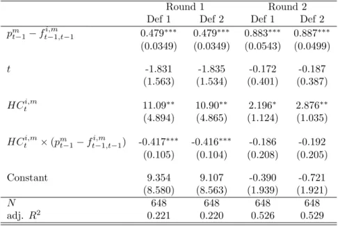
signif-icantly different from zero. Thus, below, instead of trying to explain the changes in the subjects’ levels of confidence, we use the subjects’ levels of confidence as an explanatory variable and relate them to the way in which subjects update their forecasts. In particular, we focus on how subjects’ forecasts of the period t price are adjusted between period t − 1 and period t. That is, we consider how f_t,ti,m− f_t−1,ti,m is related to the prior level of confidence, wi,m_t−1,t, and the accuracy of forecasts in previous periods relative to the realized price pm

t−1− f i,m t−1,t−1.

(29)

Table 5: Forecast adjustments: the dependent variable is f_t,ti,m− f_t−1,ti,m . Round 1 Round 2 Def 1 Def 2 Def 1 Def 2 pmt−1− f i,m t−1,t−1 0.479∗∗∗ 0.479∗∗∗ 0.883∗∗∗ 0.887∗∗∗ (0.0349) (0.0349) (0.0543) (0.0499) t -1.831 -1.835 -0.172 -0.187 (1.563) (1.534) (0.401) (0.387) HC_ti,m 11.09∗∗ _10.90∗∗ _2.196∗ _2.876∗∗ (4.894) (4.865) (1.124) (1.035) HC_ti,m× (pm t−1− f i,m t−1,t−1) -0.417∗∗∗ -0.416∗∗∗ -0.186 -0.192 (0.105) (0.104) (0.208) (0.205) Constant 9.354 9.107 -0.390 -0.721 (8.580) (8.563) (1.939) (1.921) N 648 648 648 648 adj. R2 0.221 0.220 0.526 0.529

∗_{p < 0.10,}∗∗_{p < 0.05,}∗∗∗_{p < 0.01}

takes a value of 1 if w_t−1,ti,m ≤ K, and 0 otherwise. Note that here we are focusing on a subject’s level of confidence regarding his forecast of the period-t price elicited in period t − 1. We consider two values for K, K = 5 (Def 1) and K = 7 (Def 2). Note that the definition of HC_ti,m differs from that of HCS_ti,m (which was based on w_t,ti,m and not on wi,m_t−1,t) presented in Section 3.3.

We conjecture that, controlling for the deviation between the realized price and the prior forecast, pm

t−1− f i,m

t−1,t−1, the adjustment of the subject’s forecast becomes smaller if the subject is confident

about his forecast (HC_ti,m = 1). In addition, we conjecture that the marginal effect of pm t−1−f

i,m t−1,t−1

on the forecast adjustment will be smaller if the subject’s level of confidence is high.

Table 5 reports the results of subjects’ fixed-effect regressions. The standard errors are corrected for the within-market clustering effect.

The positive and statistically significant coefficients of pm t−1−f

i,m

t−1,t−1in both Round 1 and Round

2, regardless of the definition of HC_ti,m, are easy to understand. If subjects have underestimated the price in the previous period, they respond by raising their forecast price for the current period. The positive and statistically significant coefficient of HC_ti,m is not what we expect. This means that, contrary to what we expect, the forecast adjustment is larger when a subject’s confidence in

(30)

his previous period forecast is high than when it is low. However, as expected, the negative and statistically significant coefficients of HC_ti,m× (pm

t−1− f i,m

t−1,t−1) in Round 1 show that the marginal

effect of the price-forecast gap on the forecast adjustment is smaller if the subject’s level of confidence is high, at least in Round 1.