HAL Id: halshs-00523448
https://halshs.archives-ouvertes.fr/halshs-00523448
Submitted on 5 Oct 2010
HAL is a multi-disciplinary open access
archive for the deposit and dissemination of sci-entific research documents, whether they are pub-lished or not. The documents may come from teaching and research institutions in France or abroad, or from public or private research centers.
L’archive ouverte pluridisciplinaire HAL, est destinée au dépôt et à la diffusion de documents scientifiques de niveau recherche, publiés ou non, émanant des établissements d’enseignement et de recherche français ou étrangers, des laboratoires publics ou privés.
Aggregating sets of von Neumann-Morgenstern utilities
Eric Danan, Thibault Gajdos, Jean-Marc Tallon
To cite this version:
Eric Danan, Thibault Gajdos, Jean-Marc Tallon. Aggregating sets of von Neumann-Morgenstern utilities. 2010. �halshs-00523448�
Documents de Travail du
Centre d’Economie de la Sorbonne
Aggregating sets of von Neumann-Morgenstern utilities
Eric DANAN, Thibault GAJDOS, Jean-Marc TALLON
Aggregating sets of von Neumann-Morgenstern
utilities
∗
Eric Danan
†Thibault Gajdos
‡Jean-Marc Tallon
§July 22, 2010
Abstract
We analyze the aggregation problem without the assumption that individu-als and society have fully determined and observable preferences. More precisely, we endow individuals and society with sets of possible von Neumann-Morgenstern utility functions over lotteries. We generalize the classical neutrality assumption to this setting and characterize the class of neutral social welfare function. This class turns out to be considerably broader for indeterminate than for determinate util-ities, where it basically reduces to utilitarianism. In particular, aggregation rules may differ by the relationship between individual and social indeterminacy. We characterize several subclasses of neutral aggregation rules and show that utilitar-ian rules are those that yield the least indeterminate social utilities, although they still fail to systematically yield a determinate social utility.
Keywords. Aggregation, vNM utility, indeterminacy, neutrality, utilitarianism. JEL Classification. D71, D81.
1
Introduction
Arrovian social choice (Arrow, 1951) deals with the question of aggregating individual preference relations over a set of social alternatives into a social preference relation over this set. The main insight of Arrow’s celebrated impossibility theorem is that there is no reasonable way to do so, unless one puts restrictions on either the domain or the
∗We thank Philippe Mongin for useful comments and discussions, as well as audience at London School of Economics, Universit´e Paris Descartes, Ecole Polytechnique, and D-TEA 2010. Financial support from ANR ComSoc (ANR-09-BLAN-0305-03) is gratefully acknowledged.
†Universit´e de Cergy-Pontoise, THEMA, 33 boulevard du Port, 95000 Cergy-Pontoise cedex, France. E-mail: Eric.Danan@u-cergy.fr.
‡CNRS, Ecole Polytechnique, CERSES. E-mail: gajdos@univ-paris1.fr.
jean-structure of individual preferences. This led Sen (1970, 1973) to move to a richer frame-work, replacing individual preferences by utility functions.1 This setting allows to
for-mulate various assumptions on the measurability and comparability of individual utility functions, the Arrovian setting corresponding to the particular “ordinal measurability, non-comparability” assumption, and to obtain possibility results under non-Arrovian as-sumptions (D’Aspremont and Gevers, 1977).2 This approach of aggregating individual
utility functions into a social preference relation has since then become the standard one in social choice theory.
In this paper we take issue with an assumption which is implicit in this standard approach: that individuals have fully determined and observable utility functions. Indeed, in many relevant situations, a social planner may be unable or unwilling to assign a determinate utility function to each individual. First, individuals themselves may envision more than one utility function, either because their preferences are incomplete (Aumann, 1962; Bewley, 1986; Dubra, Maccheroni, and Ok, 2004; Evren and Ok, 2010), or because they are uncertain about their tastes (Koopmans, 1964; Kreps, 1979; Dekel, Lipman, and Rustichini, 2001; Cerreia-Vioglio, 2009), or because they are driven by several “selves” or “rationales” (May, 1954; Kalai, Rubinstein, and Spiegler, 2002; Ambrus and Rozen, 2009; Green and Hojman, 2009). Second, the “individuals” under consideration may in fact be group of individuals, such as households, and the social planner may then want to remain agnostic on how individual utilities are aggregated within such groups. Third, even if all individuals have single, fully determined utility functions, the social planner may only partially observe them (Manski, 2005, 2010).
In order to account for such situations, we endow individuals with sets of utility functions. Such a set represents the possible utility functions this individual may have, according to the social planner. The particular case where this set is a singleton then corresponds to the standard setting in which the individual has a single, fully determined utility function. We shall say that the individual’s utility function is determinate in this case and indeterminate otherwise, to summarize the different situations mentioned above.
1.1
The aggregation problem
How can indeterminate utilities be aggregated? Although one might find it desirable that the social planner settle for a fully determined social preference relation in all situations, one can also conceive that the indeterminacy of individual utilities sometimes prevent her to do so. In fact, even in situations where all individuals have fully determined util-ity functions, a social planner could leave the social preference relation indeterminate in
1To be precise, Sen used the term “individual welfare function”. Although this terminology is more rigorous, we will follow the usual one. A discussion of the interpretation of utility in social choice can be found in Mongin and D’Aspremont (1998).
order to avoid inter-personal utility comparisons. Thus, in order to allow for all these possibilities, it seems natural to consider the general problem of aggregating individual sets of utility functions into a social set of preference relations (or, equivalently, an in-complete social preference relation), the particular case where this latter set is a singleton corresponding to fully determined social preferences.
This approach, however, encounters a major difficulty that we now explain. Virtually all the possibility results for determinate utilities are obtained by means of a “neutral-ity” assumption, according to which the social relative ranking between two alternatives only depends on their respective utility levels for all individuals.3 This assumption
con-siderably simplifies the analysis because it basically boils the aggregation rule down to a social preference relation over vectors of individual utility levels. Various additional assumptions then characterize specific aggregation rules.
Now, when a utility function is indeterminate, so is, in general, the utility level of an alternative. In other words, alternatives now have sets of possible utility levels, which may or may not be singletons. This renders the neutrality assumption, now meaning that the social relative ranking between two alternatives only depends on their respective sets of utility levels for all individuals, much less reasonable. To illustrate this point, consider two alternatives x and y and the sets of utility functions U = {u1, u2, u3} and
U0 = {u
1, u2, u4}, where the utility functions u1, u2, u3, and u4are defined by the following
table.
u1 u2 u3 u4
x 1 0 1 0 y 1 0 0 1
For both sets of utility functions, the set of utility levels of both alternatives is {0, 1}. Where the two sets of utility functions differ is in the “correlation” between the utility levels of x and y. In fact, according to U, x is clearly at least as good as y and possibly better whereas, according to U0, this pattern is reversed. Nevertheless, under the
neutral-ity assumption, the social relative ranking between x and y must be the same whether all individuals have the same set of utility functions U or all have the same set of utility functions U0, for instance. More generally, since sets of utility levels do not keep track
of utility “correlations”, neutrality implies that social preferences cannot take them into account either, which is clearly an undesirable feature.
Our solution to this difficulty is to depart one step further from the standard approach by considering aggregation of individual sets of utility functions into a social set of utility functions rather than a social set of preference relations. In other words, we put heavier weight on the social planner’s shoulders who must now not only determine the possible
3This assumption is usually decomposed into an “independence of irrelevant alternatives” assumption and a “Pareto indifference” assumption, see below for formal definitions.
social preference relations but also pin down the corresponding social utility functions. This setting enables us to impose the following neutrality assumption: the social set of utility levels of an alternative only depends on its sets of utility levels for all individuals. This requirement (which ignores utility “correlations” at both the individual and social level) is a reasonable one and, at the same time, makes the aggregation problem tractable by inducing a mapping from vectors of individual sets of utility levels into social sets of utility levels.
We also put restrictions on the domain and structure of individual and social sets of utility functions. Namely, we take alternatives to be lotteries and restrict attention to sets of von Neumann-Morgenstern (vNM) utility functions. This is, first, a salient setting in decision and social choice theory and, furthermore, one in which the benchmark case of determinate utilities (i.e. singleton sets of utility functions) is remarkably simple. Indeed, Coulhon and Mongin (1989) have shown that if both individuals and society are assumed to have determinate vNM utility functions then neutrality alone implies that the social utility function must be an affine transformation of the individual utility functions.4 The
intuition behind this result is that, under neutrality, the affinity property of vNM utility functions directly implies affinity of the aggregation rule. A standard “Pareto preference” assumption then suffices to make the coefficients of the affine transforamtion non-negative, i.e. yield utilitarianism.5 Thus, for determinate vNM utilities over lotteries, the class of
neutral aggregation rules “almost” reduces to that of utilitarian ones.6
1.2
Outline and summary of results
Section 2 introduces the formal setup. We let X denote the set of alternatives (lotteries) and P denote the set of compact and convex sets of (vNM) utility functions. Given such a set U of utility functions, the set U(x) of possible utility levels of an alternative x is then a compact interval and we refer to it as the utility interval of x. Finally, we let I denote the finite set of individuals and consider a social welfare function F associating to each profile (Ui)i∈I of individual sets of utility functions a social set of utility functions
F ((Ui)i∈I). We restrict attention to the case where X is the set ∆(Z) of simple lotteries
over some set Z of social outcomes and the domain of F is the set of all possible profiles of sets of (vNM) utility functions, until Section 6 in which we will show that our results hold for more general alternatives and domains.
4Coulhon and Mongin’s result is a “multi-profile” version of Harsanyi (1955)’s celebrated aggregation theorem, which is a “single-profile” result. As they discuss, the “multi-profile” approach has several ad-vantages over the “single-profile” one, notably uniqueness of the coefficients of the affine transformation. 5By “utilitarianism” we mean what is sometimes referred to as “generalized utilitarianism”, i.e. social utility being an affine transformation of individual utilities with non-negative coefficients.
6For determinate utilities over arbitrary alternatives, in contrast, additional assumptions are needed to characterize different classes of neutral aggregation rules. To characterize utilitarianism, in particular, a “cardinal measurability, unit comparability” and a “continuity” assumption must be added (Blackorby, Donaldson, and Weymark, 1984).
Our first task, in Section 3, is to provide a characterization of neutral social welfare functions in our setting of (possibly) indeterminate vNM utilities. This turns out to be substantially more difficult than in the benchmark case of determinate utilities, mainly because vNM utility intervals do not in general enjoy the affinity property of vNM utility functions. They do nevertheless satisfy (weaker) convexity properties and we are therefore able to characterize the class of neutral social welfare functions (Theorem 1). Namely, neutrality is equivalent to the following relationship between the individual and social utility intervals: for some compact and convex set Φ ⊂ (RI
+)2×R, F ((Ui)i∈I)(x) = [ (α,β,γ)∈Φ X i∈I αiUi(x) − X i∈I βiUi(x) + γ ! .
This is our most general result and many interesting corollaries follow from it. It pins down the social utility interval as the union of a set of affine transformations of all in-dividual utility intervals, each affine transformation corresponding to a weight-constant vector (α, β, γ) ∈ Φ. Each individual i’s utility interval enters twice in each affine trans-formation, once with a non-negative coefficient αi and once with a non-positive coefficient
βi. This duality of individual weights generalizes the benchmark case of determinate
util-ities in which individual utility levels enter only once in the affine transformation but coefficients have no sign restriction and, accordingly, disappears if an additional “Pareto preference” assumption (or, equivalently, a strengthening of the neutrality assumption) is imposed. Indeed, the above relationship then reduces to the following one (Corollary 1): for some compact and convex set Ω ⊂RI
+×R, F ((Ui)i∈I)(x) = [ (θ,γ)∈Ω X i∈I θiUi(x) + γ ! .
Even under these stronger assumptions, the class of neutral social welfare functions is considerably broader for indeterminate than for determinate utilities. Indeed, first, dif-ferent neutral welfare functions may differ by the size of the set Ω of weight-constant vector, a larger Ω corresponding to a social planner who “generates” more indeterminacy (whether individual utilities are determinate or not). Second, the latter relationship only pins down the social utility intervals and this does not fully determine the social set of utility functions, as explained above, so that different neutral social welfare functions may differ in terms of social utility “correlations” even if they share the same Ω.
Our goal, from then on, is to explore the class of neutral social welfare functions and characterize various interesting subclasses. Section 4 is concerned with the first of the two dimensions mentioned above, the relationship between individual and social in-determinacy. In particular, we obtain the following important consequence of Theorem 1 (Corollary 2): under neutrality, for the social utility function to be determinate, it
is necessary that all individual utility functions be determinate as well (except for in-dividuals that are “irrelevant” to the social planner). Thus, the social planner cannot “resolve” individual indeterminacy. The best she can do, then, is to “preserve” individual determinacy by adopting a determinate social utility function whenever all individuals have determinate utility functions. Adding this “determinacy preservation” requirement characterizes the particular case where the set Ω above is a singleton (Corollary 3), i.e. for some θ ∈RI + and some γ ∈R, F ((Ui)i∈I)(x) = X i∈I θiUi(x) + γ.
We call such aggregation rules locally utilitarian since they correspond to utilitarian ag-gregation of individual utility intervals (but not necessarily of individual sets of utility functions, as explained above). Among neutral aggregation rules, locally utilitarian ones are those who do not avoid inter-personal utility comparisons and only exhibit social indeterminacy in situations of individual indeterminacy. In contrast, a prominent aggre-gation rule that is neutral but not locally utilitarian is the unanimity rule, which takes as social set of utility functions the (convex hull of the) union of all individual sets of utility functions. This rule corresponds to the Pareto dominance relation or, in other words, to a social planner who systematically “generates” social indeterminacy rather than making inter-personal utility comparisons. Note that this rule still satisfies a weak “determinacy preservation” property: there exists at least some profile of determinate individual utili-ties for which social utility is determinate as well (namely, here, any profile in which all individuals have the same, determinate utility function). Weakening the “determinacy preservation” requirement in this way characterizes the particular case where the set Ω of weight-constant vectors can be decomposed into a set of weight vectors and a single constant (Corollary 4), i.e. for some compact and convex set Θ ⊂RI
+and a some number
γ ∈R such that, for all (Ui)i∈I ∈ D and all x ∈ X,
F ((Ui)i∈I)(x) = [ θ∈Θ X i∈I θiUi(x) ! + γ.
We call such aggregation rules locally multi-utilitarian and, under a mild “normalization” assumption, we obtain the class of normalized multi-utilitarian rules for which Θ ⊆ ∆(I). This class is bounded at one end by the normalized locally utilitarian rules corresponding to Θ being a singleton, which are those yielding the least indeterminate social utilities, and at the other end by the local unanimity rules (i.e. social welfare functions yielding the same utility intervals as the unanimity rule) corresponding to Θ = ∆(I), which are those yielding the most indeterminate social utilities.
of different aggregation rules yielding the same social utility intervals but differing in social utility “correlations”. Utility intervals, as explained above, do not convey enough information to establish a relative ranking of alternatives and, for this reason, the “local” characterization results obtained so far are not sufficient to help a social planner choose an aggregation rule. In order to fully pin down the social set of utility functions, an assumption that takes utility “correlations” into account is needed. We provide such an assumption, in the form of a strengthening of the neutrality assumption, and show that, provided the set Z of outcomes is infinite, adding it to the assumptions characterizing local multi-utilitarian rules characterizes the class of rules that are fully multi-utilitarian (Theorem 2), i.e. defined by
F ((Ui)i∈I) = [ θ∈Θ X i∈I θiUi ! + γ.
Similarly, adding this strengthening of the neutrality assumption to the assumptions characterizing local utilitarianism characterizes the class of rules that are fully utilitarian (Corollary 5), i.e. defined by
F ((Ui)i∈I) =
X
i∈I
θiUi + γ.
This latter characterization sheds a new light on the normative appeal of utilitarian aggregation rules: when individual and social utilities may possibly be indeterminate, utilitarianism is underlain not only by neutrality and “Pareto preference” assumptions (as in the benchmark case of determinate utilities) but also by a “determinacy preservation” assumption according to which social utility should be determinate whenever possible (i.e. whenever all individual utilities are themselves determinate).
Finally, Section 6 extends our characterization results to more general alternatives and domains. To this end, we adopt the “mixture space” framework (Herstein and Milnor, 1953) and show that our results hold for a large class of such spaces, including lotteries with continuous densities or opportunity sets of lotteries, for instance. We also show that our result apply to smaller domains than the full (vNM) domain considered so far, by identifying general properties of the domain that are sufficient for the results to holds. As a consequence of these extensions, we are able to show that our characterizations of (full) utilitarianism and multi-utilitarianism remain valid if the set Z of outcomes is finite, provided that the utility of some alternative with “full support” in Z is normalized to a determinate level for all individuals.
2
Setup
Let X be a non-empty set of social alternatives. We assume that X is the set ∆(Z) of simple lotteries (i.e. probability distributions with finite support) on some non-empty set Z of social (sure) outcomes. Given two alternatives x, y ∈ X and a number λ ∈ [0, 1], we define the λ-mixture of x and y, denoted xλy, by xλy = λx + (1 − λ)y (clearly, then, xλy ∈ X). We will maintain this assumption on X and use this definition of mixture until Section 6, in which we will consider more general alternatives and mixtures.
A utility function on X is a function u : X →R associating to each alternative x ∈ X a utility level u(x) ∈ R. A utility function u on X is said to be a vNM utility function if u(xλy) = λu(x) + (1 − λ)u(y) for all x, y ∈ X and all λ ∈ [0, 1].7 Let P ⊆RX denote
the set of all vNM utility functions on X. P is a linear subspace of RX and contains
all constant functions. Given a real number γ ∈R, we abuse notation by also letting γ denote the corresponding constant function in P .
We consider non-empty sets of utility functions, i.e. non-empty subsets of RX. Our
interpretation of such a set is that the utility function may possibly be any member of the set, without further information being available. We say that the utility function is determinate if the set is a singleton and indeterminate otherwise. We restrict attention to sets of vNM utility functions. Let P denote the set of all non-empty, compact, and convex subsets of P , where P is endowed with the subspace topology and RX with the
product topology. Note that P contains in particular all convex hulls of finite sets of vNM utility functions on X and, hence, all singletons.
When the utility function is indeterminate, an alternative does not in general have a single utility level but rather a set (in fact, a non-empty and compact interval) of possible utility levels. Given a set U ∈ P of utility functions and an alternative x ∈ X, let U(x) = {u(x) : u ∈ U} denote this utility interval. Clearly, a set U ∈ P of utility functions is a singleton if and only if the utility interval U(x) is a singleton for all x ∈ X and, in this case, knowing the set U of utility functions is equivalent to knowing the utility interval U(x) for all x ∈ X. In the general case of a non-singleton set of utility functions, however, this is no longer true: a set of utility functions determines all utility intervals but the converse does not necessarily hold, as observed in the introduction. In other words, there are distinct sets of utility functions that yield the same utility intervals for all alternatives.
Let I be a non-empty and finite set of individuals. Given a non-empty domain D ⊆ PI, an social welfare function F : D → P associates to each profile (U
i)i∈I of individual
sets of utility functions a social set U = F ((Ui)i∈I) of utility functions. We will maintain
7Given our assumption on X and definition of mixture, the two following are equivalent: (i) u is a vNM utility function, (ii) u(x) =P
z∈Zx(z)u(z) for all x ∈ X. However, only (i) is still well-defined in the more general setting that we will consider in Section 6, hence the use of (i) rather than (ii) which is more usual in the current setting, for the definition of a vNM utility function.
the assumption that D = PI from now on, and will relax it in Section 6.
3
Neutrality
In this Section, we first introduce a neutrality assumption for indeterminate utilities and characterize the class of social welfare functions satisfying this assumption. This leads to identifying three dimensions along which this characterization generalizes the one obtained by Coulhon and Mongin (1989) in the particular case where both individual and social utilities are determinate. We then elaborate on this and study to what extent these generalizations are robust to a strengthening of the neutrality assumption.
3.1
A characterization: interval neutrality
Our first contribution is to characterize neutral social welfare functions in our setting of indeterminate utilities. To this end, we start by generalizing the classical Independence of Irrelevant Alternatives and Pareto Indifference axioms which are the two components of neutrality for determinate utilities. Considering utility intervals rather than utility levels naturally leads to the following generalizations.
Axiom 1 (Interval Independence of Irrelevant Alternatives). For all (Ui)i∈I, (Ui0)i∈I ∈ D
and all x ∈ X, if Ui(x) = Ui0(x) for all i ∈ I then F ((Ui)i∈I)(x) = F ((Ui0)i∈I)(x).
Axiom 2 (Interval Pareto Indifference). For all (Ui)i∈I ∈ D and all x, y ∈ X, if Ui(x) =
Ui(y) for all i ∈ I then F ((Ui)i∈I)(x) = F ((Ui)i∈I)(y).
Axiom 3 (Interval Pareto Weak Preference). For all (Ui)i∈I ∈ D and all x, y ∈ X, if
Ui(x) ≥ Ui(y) for all i ∈ I then F ((Ui)i∈I)(x) ≥ F ((Ui)i∈I)(y).8
Interval Independence of Irrelevant Alternatives expresses the fact that if a given al-ternative has the same utility interval for all individuals according to two different profiles of individual sets of utility functions, then it also has the same utility interval according to the two corresponding social sets of utility functions. Interval Pareto Indifference, on the other hand, states that if two alternatives have the same utility interval for all indi-viduals according to a given profile of individual sets of utility functions, then they also have the same utility interval according to the corresponding social set of utility func-tions. Interval Pareto Weak Preference is an obvious strengthening of Interval Pareto Indifference.
Remark 1. An alternative generalization of the classical Pareto Indifference axiom would be Pointwise Pareto Indifference: for all (Ui)i∈I ∈ D and all x, y ∈ X, if ui(x) = ui(y)
for all i ∈ I and all ui ∈ Ui then u(x) = u(y) for all u ∈ F ((Ui)i∈I). Similarly, we
could have stated a pointwise rather than interval version of the Pareto Weak Preference axiom. Given Interval Independence of Irrelevant Alternatives, these pointwise versions of the Pareto axioms are stronger than the corresponding interval versions. As it turns out, the weaker interval versions that we use are sufficient for our results.
Since D = PI, the conjunction of Interval Independence of Irrelevant Alternatives
and Interval Pareto Indifference is equivalent to the following interval neutrality prop-erty: for all (Ui)i∈I, (Ui0)i∈I ∈ D and all x, y ∈ X, if Ui(x) = Ui0(y) for all i ∈ I then
F ((Ui)i∈I)(x) = F ((Ui0)i∈I)(y). Interval neutrality reflects the fact that the social utility
interval is fully determined by all individual utility intervals, independently of the par-ticular profile and alternative that yield these individual utility intervals. Equivalently, there exists a (unique) function G : KI → K , where K denotes the set of all non-empty
and compact real intervals, such that F ((Ui)i∈I)(x) = G((Ui(x))i∈I) for all (Ui)i∈I ∈ D
and all x ∈ X. As for determinate utilities, restricting attention to vNM utility functions imposes some structure on this function G. However, since we work with sets of utility functions rather than single utility functions, this structure turns out to be weaker than affinity of G. The structure of this function is given in the following characterization of interval neutral social welfare functions.
Theorem 1. Assume X = ∆(Z) with |Z| ≥ 2 and D = PI. Then a social welfare
function F satisfies Interval Independence of Irrelevant Alternatives and Interval Pareto Indifference if and only if there exists a non-empty, compact, and convex set Φ ⊂ (RI
+)2×R
such that, for all (Ui)i∈I ∈ D and all x ∈ X,
F ((Ui)i∈I)(x) = [ (α,β,γ)∈Φ X i∈I αiUi(x) − X i∈I βiUi(x) + γ ! . (1)
Moreover, Φ can be taken such that (1) holds for some non-empty, compact, and convex set Φ0 ⊂ (RI
+)2×R if and only if Φ ⊆ Φ0 ⊆ {(α − η, β − η, γ) : (α, β, γ) ∈ Φ, η ∈RI+}.
Thus a social welfare function F is interval neutral if and only if the social utility interval is the union of a set of affine transformations of all individual utility intervals, with individual i’s utility interval entering twice in each affine transformation, once with a non-negative coefficient αi and once with a non-positive coefficient −βi. Moreover, the
set Φ of weight-constant vectors (α, β, γ) is “almost” unique in the sense that, first, there exists a unique Φ that is minimal with respect to set inclusion and, second, another set Φ0 satisfies (1) if and only if it consists in the minimal Φ to which are added
weight-constant vectors that are always irrelevant to the social utility interval. Indeed, it is easily checked that, for all utility interval Ui(x), if αi ≥ αi− ηi ≥ 0 and βi ≥ βi− ηi ≥ 0
3.2
Discussion
How does Theorem 1 compare with the characterization of neutrality obtained by Coulhon and Mongin (1989) in the particular case where both individual and social utilities are determinate? A natural extension of their characterization to sets of utility functions would be that, for some θ ∈RI and γ ∈R,
F ((Ui)i∈I) =
X
i∈I
θiUi + γ. (2)
There are three dimensions along which (1) is more general than (2):
(i) whereas (2) fully pins down the social set of utility functions, (1) only pins down all social utility intervals,
(ii) in (1) the social utility interval is made of several affine transformations of all individual utility intervals, rather than a single one as in (2),
(iii) in (1) each individual i’s utility interval enters twice in each affine transformation rather than once (so (2) corresponds to the particular case where either αi = 0 or
βi = 0).
Therefore, the class of interval neutral social welfare functions is substantially broader for indeterminate utilities than for determinate utilities.
As we will see shortly, the first two dimensions are robust to a strengthening of Interval Pareto Indifference whereas the third one is not. We thus defer the illustration of the first two points to section 3.4 and only comment on the third point now.
To illustrate this point, let I = {1, 2} and consider the two social welfare functions F1(U1, U2) = U1 + U2 and F2(U1, U2) = 2(U1+ U2) − (U1 + U2), which obviously satisfy
(1). F1 uses only one weight per individual whereas F2 uses two. These two functions
agree if both U1(x) and U2(x) are singletons, but otherwise F1 yields a smaller utility
interval than F2. For instance, F1([0, 1], [0, 1]) = [0, 2] ⊂ [−2, 4] = F2([0, 1], [0, 1]).
More generally, for any social welfare function F satisfying (1), we have
F ((Ui)i∈I)(x) = [ (α,β,γ)∈Φ ( X i∈I (αiui(x) − βivi(x)) + γ : ui, vi ∈ Ui, i ∈ I ) ⊇ [ (α,β,γ)∈Φ ( X i∈I (αi− βi) ui(x) + γ : ui ∈ Ui, i ∈ I ) = [ (α,β,γ)∈Φ X i∈I (αi− βi) Ui(x) + γ ! ,
where, in general, equality holds if and only if Ui(x) is a singleton for all i ∈ I. Thus,
allowing for two weights per individual rather than a single one brings in social welfare functions yielding larger utility intervals.
3.3
Sketch of the proof
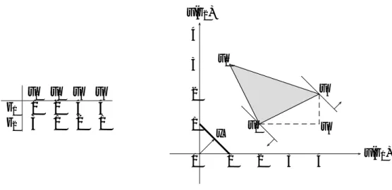
Before providing a brief sketch of the proof of Theorem 1, it is useful to gain insight into the structure of vNM utility intervals. To this end consider the example represented in Figure 1. The set of outcomes is Z = {z1, z2}. The left-hand side table defines utility
functions u1, u2, u3, u4 ∈ P (of course, a vNM utility function u ∈ P is affine and, hence,
fully determined by u(z1) and u(z2)). These utility functions are depicted on the
right-hand side graph, in which the thick horizontal segment represents the set X = ∆(Z) of alternatives and the utility level of each alternative x ∈ X is measured along the corresponding vertical axis.
The set U = conv({u1, u2, u3}) of utility functions (i.e. all convex combinations of u1,
u2, and u3) fills the shaded area on the graph.9 The utility interval U(x) of an alternative
x ∈ X corresponds to the intersection of the corresponding vertical axis with this shaded area. The set U0 = conv({u
1, u2, u3, u4}) of utility functions fills the same shaded area on
the graph, so that we have U0(x) = U(x) for all x ∈ X, although we clearly have U0 6= U
since u4 ∈ U. As explained above, this is because U and U/ 0 only differ in terms of utility
“correlations”: in both sets of utility functions it is possible that the utility level of z1 be
equal to 4 and it is also possible that the utility level of z2 be equal to 1, but in U0 these
two possibilities may arise from the same utility function whereas in U they cannot. Two key properties of utility intervals also appear from the graph of the set U (or, equivalently, U0) of utility functions. First, although affinity of vNM utility functions
does not extend to utility intervals, in the sense that one would have U(xλy) = λU(x) + (1 − λ)U(y), an inclusion relation nevertheless holds, namely U(xλy) ⊆ λU(x) + (1 − λ)U(y). Equivalently, the function x 7→ max U(x) is convex and the function x 7→ min U(x) is concave. Second, although the shaded area on the graph is not convex, it still contains all line segments joining the maximum of a utility interval with the minimum of another utility interval, i.e. λ max U(x) + (1 − λ) min U(y) ∈ U(xλy). This establishes a relationship between the two functions just defined. These two properties turn out to be general properties of sets of (vNM) utility functions (see Lemma 1 in the appendix).
The “if” part of Theorem 1 is straightforward. To prove the “only if” part, first note that, from interval neutrality, we know that F ((Ui)i∈I)(x) ∈ K is a function of
(Ui(x))i∈I ∈ K I. Equivalently, both max F ((Ui)i∈I)(x) ∈ R and min F ((Ui)i∈I)(x) ∈
R are functions of (max Ui(x), min Ui(x))i∈I ∈ (RI)2. These functions are not
neces-sarily affine but the two properties of utility intervals mentioned above nevertheless
u1 u2 u3 u4 z1 1 2 4 4 z2 3 1 2 1 z1 x z2 u(z1) u(z2) u1 3 u2 4 u3 u4 1 4 2 1 2 3 u(x)
Figure 1: Example of set of utility functions
imposes some structure on them. Most importantly, the first property implies that max F ((Ui)i∈I)(x) is convex, non-decreasing in each max Ui(x), and non-increasing in each
min Ui(x). Symmetrically, min F ((Ui)i∈I)(x) is concave, non-decreasing in each min Ui(x),
and non-increasing in each max Ui(x). The second property implies that the two functions
are also Lipschitzian and have “asymptotic” relationships with each other. From these and other properties, using results from convex analysis, we can construct a common, compact set Φ ⊂ (RI
+)2×R such that
max F ((Ui)i∈I)(x) = max (α,β,γ)∈Φ X i∈I αimax Ui(x) − X i∈I βimin Ui(x) + γ ! ,
min F ((Ui)i∈I)(x) = min (α,β,γ)∈Φ X i∈I αimin Ui(x) − X i∈I βimax Ui(x) + γ ! , which is equivalent to (1).
3.4
Strengthening Interval Pareto Indifference
What is the effect of strengthening Interval Pareto Indifference to Interval Pareto Weak Preference in Theorem 1? In the particular case of determinate utilities, in which neutral-ity yields one weight per individual, Pareto Weak Preference ensures that all weights are non-negative. Similarly, in the general case of indeterminate utilities, in which interval neutrality yields one non-negative and one non-positive weight per individual, Interval Pareto Weak Preference ensures that all non-positive weights are null. Indeed, for an interval neutral social welfare function F , Interval Pareto Weak Preference means that max F ((Ui)i∈I)(x) and min F ((Ui)i∈I)(x) are both non-decreasing in each max Ui(x) and
each min Ui(x). In particular, the maximum of the social utility interval must be
non-decreasing in the minimum of each individual’s utility interval, which implies that all β coefficients must be equal to zero in (1).
To prove this implication, fix two distinct alternatives x, y ∈ X and a real number µ > 0 and consider, for each individual i ∈ I, a set Ui ∈ P of utility functions such
that Ui(x) = {0} and Ui(y) = [−µ, 0]. Interval Pareto Weak Preference then implies
max F ((Ui)i∈I)(x) ≥ max F ((Ui)i∈I)(y), i.e. max(α,β,γ)∈Φγ ≥ max(α,β,γ)∈Φ(µ
P
i∈iβi + γ)
by (1). Since this inequality must hold for any µ > 0, we must then have P
i∈iβi ≤ 0,
i.e. β = 0 since β ∈RI
+, for all (α, β, γ) ∈ Φ.
Given the uniqueness part of Theorem 1, setting all β coefficients to 0 fully pins down Φ. We thus obtain the following result.
Corollary 1. Assume X = ∆(Z) with |Z| ≥ 2 and D = PI. Then a social welfare
function F satisfies Interval Independence of Irrelevant Alternatives and Interval Pareto Weak Preference if and only if there exists a non-empty, compact, and convex set Ω ⊂ RI
+×R such that, for all (Ui)i∈I ∈ D and all x ∈ X,
F ((Ui)i∈I)(x) = [ (θ,γ)∈Ω X i∈I θiUi(x) + γ ! . (3) Moreover, Ω is unique.
Thus, as for determinate utilities, Interval Pareto Weak Preference fixes the sign of individual weights. In so doing, it also yields a single weight per individual rather than two and, thereby, fills part of the identified gap between interval neutrality and utilitarianism (defined as (2) with θ ∈RI
+) that arises from indeterminacy of utilities.
As explained above, there remain two dimensions along which (3) is more general than utilitarianism. The first one is that (3) pins down all social utility intervals but not the social set of utility functions. To illustrate this point, consider the social welfare functions F1((Ui)i∈I) = Pi∈IUi and F2((Ui)i∈I) = {u ∈ P : u(x) ∈ Pi∈IUi(x) for all x ∈ X}.
Then the two functions satisfy (1) and yield the same social utility intervals, but they yield different sets of utility functions and, in fact, only F1 is utilitarian. For instance,
if Ui = [0, 1] for all i ∈ I, so that all individual sets of utility functions are made of
constant functions only, then F2((Ui)i∈I) = {u ∈ P : u(z) ∈ [0, |I|] for all z ∈ Z} contains
non-constant functions.10
The second dimension along which (3) is more general than utilitarianism is that in (3) the social set of utility functions may contain more than one affine transformation of all individual sets of utility functions. To illustrate this point, consider the unanimity rule F ((Ui)i∈I) = conv(Si∈IUi), which simply corresponds to the Pareto dominance
relation. For this rule, the social set of utility functions can equivalently be expressed as F ((Ui)i∈I) =Sθ∈∆(I)
P
i∈IθiUi and, hence, is the union of a set of utilitarian rules.
10Note that this instance also shows that F
2 does not satisfy Pointwise Pareto Weak Preference or even Indifference, although it does satisfy Interval Pareto Weak Preference.
3.5
An alternative characterization: max-min neutrality
Corollary 1 reduces (1) to (3) by strengthening Interval Pareto Indifference while keeping Interval Independence of Irrelevant Alternatives. An alternative axiomatization of (3) consists in strengthening Interval Independence of Irrelevant Alternatives while keeping Interval Pareto Indifference. Namely, consider the following Max-Min Independence of Irrelevant Alternatives axiom: for all (Ui)i∈I, (Ui0)i∈I ∈ D and all x ∈ X,
(i) if max Ui(x) = max Ui0(x) for all i ∈ I then max F ((Ui)i∈I)(x) = max F ((Ui0)i∈I)(x),
(ii) if min Ui(x) = min Ui0(x) for all i ∈ I then min F ((Ui)i∈I)(x) = min F ((Ui0)i∈I)(x).
Since D = PI, the conjunction of Max-Min Independence of Irrelevant Alternatives and
Interval Pareto Indifference is equivalent to the following max-min neutrality property: for all (Ui)i∈I, (Ui0)i∈I ∈ D and all x, y ∈ X,
(i) if max Ui(x) = max Ui0(y) for all i ∈ I then max F ((Ui)i∈I)(x) = max F ((Ui0)i∈I)(y),
(ii) if min Ui(x) = min Ui0(y) for all i ∈ I then min F ((Ui)i∈I)(x) = min F ((Ui0)i∈I)(y).
Max-min neutrality expresses the fact that the maximum of the social utility interval is fully determined by the maximum of all individual utility intervals whereas the minimum of the social utility interval is fully determined by the minimum of all individual utility intervals, which strengthens interval neutrality and, hence, implies (1).
It turns out that max-min neutrality is in fact equivalent to (3), i.e. to the conjunction of Interval Independence of Irrelevant Alternatives and Interval Pareto Weak Preference. Indeed, on the one hand, (3) is equivalent to
max F ((Ui)i∈I)(x) = max (θ,γ)∈Ω X i∈I θimax Ui(x) + γ ! ,
min F ((Ui)i∈I)(x) = min (θ,γ)∈Ω X i∈I θimin Ui(x) + γ ! ,
and, hence, implies max-min neutrality. On the other hand, recall that interval neutrality implies that max F ((Ui)i∈I)(x) is non-decreasing in each max Ui(x) and non-increasing in
each min Ui(x) whereas min F ((Ui)i∈I)(x) is non-decreasing in each min Ui(x) and
non-increasing in each max Ui(x). From there, Max-Min Independence of Irrelevant
Alterna-tives has the same effect as Interval Pareto Weak Preference: it eliminates the dependency of the social maximum on each individual minimum as well as the dependency of the so-cial minimum on each individual maximum and, thereby, yields (3). Thus, (3) can be derived from neutrality axioms alone, without appealing to Pareto preference axioms.
4
Individual and social indeterminacy
Allowing both individual and social utilities to be indeterminate raises the question of the relationships between individual and social indeterminacy. More precisely, we may ask the following questions:
(i) Given a social welfare function and a profile of individual sets of utility functions, does indeterminacy of individual utilities cause indeterminacy of social utility? (ii) Given a social welfare function, if individual utilities are more indeterminate in a
profile than in another, is it so for social utility as well?
(iii) Given a profile of individual utilities, when is social utility more indeterminate for a social welfare function than another?
We will examine these three questions within the class of social welfare functions identified in Corollary 1. Providing answers to these questions will lead us to identify further conditions, which strengthen the characterization obtained in (3) but still fall short of characterizing utilitarianism.
4.1
Does individual indeterminacy cause social indeterminacy?
We tackle here the first question and consider a social welfare function F satisfying (3) and a profile (Ui)i∈I ∈ D. For a given alternative x ∈ X, a necessary condition for the
social utility interval F ((Ui)i∈I)(x) to be a singleton is that for each vector (θ, γ) ∈ Ω, the
corresponding affine transformation of utility intervalsP
i∈IθiUi(x) + γ be a singleton as
well. This necessary condition, in turn, can only be satisfied if each individual i’s utility interval Ui(x) is itself a singleton, unless θi = 0, in which case individual i is “irrelevant”
in this affine transformation. Thus, if all individuals are “relevant” then the social utility level are determinate only if all individual utility levels are themselves determinate.
To formalize this point, say that an individual i ∈ I is interval null if, for all (Uj)j∈I, (Uj0)j∈I ∈ D and all x ∈ X, F ((Uj)j∈I)(x) = F ((Uj0)j∈I)(x) whenever Uj(x) =
U0
j(x) for all j ∈ I \ {i}. This reflects the idea that individual i is completely “irrelevant”
to the social planner. For a social welfare function satisfying (3), an individual i ∈ I is interval null if and only if θi = 0 for all (θ, γ) ∈ Ω. The “if” part of this statement is
straightforward. To prove the “only if” part, assume individual i ∈ I is interval null, fix a real number µ > 0, and consider the sets of utility functions Ui = {µ}, Ui0 = {0}, and
Uj = Uj0 = {0} for all j ∈ I \ {i}. Since i is interval null, we then have, for all x ∈ X,
max F ((Ui)i∈I)(x) = max F ((Ui0)i∈I)(x), i.e. max(θ,γ)∈Ω(µθi + γ) = max(θ,γ)∈Ωγ by (3).
Since this inequality must hold for all µ > 0, we must then have θi ≤ 0, i.e. θi = 0 since
θ ∈RI
Hence, for all (Ui)i∈I ∈ D and all x ∈ X, if F ((Ui)i∈I)(x) is a singleton then, for all
i ∈ I, either Ui(x) is a singleton or i is interval null. Since a set U of utility functions is
a singleton if and only if the utility interval U(x) is a singleton for all x ∈ X, we then obtain the following result.
Corollary 2. Assume X = ∆(Z) with |Z| ≥ 2 and D = PI. Let F be a social welfare
function satisfying (3). Then for all (Ui)i∈I ∈ D, if F ((Ui)i∈I) is a singleton then, for all
i ∈ I, either Ui is a singleton or i is interval null.
Thus, if all individuals are “relevant” then the social utility function can only be de-terminate if all individual utility functions are themselves dede-terminate. Society cannot “resolve” individual indeterminacy. For example, one may find it desirable that society selects a profile (ui)i∈I of individual utility functions out of each profile (Ui)i∈I of
indi-vidual sets of utility functions and use some affine transformation P
i∈Iθiui + γ of the
selected individual utility functions as the (determinate) social utility function, but this is incompatible with the axioms of Corollary 1, unless θ = 0. This point, in fact, only relies on interval neutrality and not on Interval Pareto Weak Preference, so if one wants society to “resolve” individual indeterminacy then one must give up the assumption that the social utility interval is fully determined by all individual utility intervals.11
The converse to Corollary 2 does not hold: even if all individual utilities are deter-minate, social utility may well be indeterminate. This is the case, for example, for the unanimity rule, which yields an indeterminate social utility function whenever all indi-viduals do not have the same, determinate utility function. A utilitarian social welfare function F ((Ui)i∈i) =Pi∈IθiUi+ γ, on the other hand, yields a determinate social utility
function whenever all individuals have determinate utility functions. The latter function always “preserves” determinacy by making inter-personal utility comparisons whereas the former, by avoiding such comparisons, sometimes “generates” indeterminacy. This raises the question of characterizing the class of all social welfare functions satisfying (3) that always “preserve” determinacy.
4.2
Local utilitarianism
The following axiom captures the fact that the social welfare function does not “generate” social indeterminacy by avoiding inter-personal utility comparisons.
Axiom 4 (Strong Determinacy Preservation). For all ({ui})i∈I ∈ D, there exists u ∈ P
such that F (({ui})i∈I) = {u}.
The effect of adding Strong Determinacy Preservation to the axioms of Corollary 1 is to reduce Ω to a singleton in (3). To prove this, let (θ, γ), (θ0, γ0) ∈ Ω. Then, letting
Ui = {0} for all i ∈ I, we have {γ, γ0} ⊆ F ((Ui)i∈I)(x) for all x ∈ X, so γ = γ0. Hence,
fixing some individual i ∈ I and letting Ui = {1} and Uj = {0} for all j ∈ I \ {i}, we
have {θi+ γ, θi0 + γ} ⊆ F ((Ui)i∈I)(x) for all x ∈ X, so θi = θi0. Since this must hold for
all i ∈ I, we must have θ = θ0, so that Ω is a singleton. We thus obtain the following
characterization.
Corollary 3. Assume X = ∆(Z) with |Z| ≥ 2 and D = PI. Then a social welfare
function F satisfies Interval Independence of Irrelevant Alternatives, Interval Pareto Weak Preference, and Strong Determinacy Preservation if and only if there exist a vector θ ∈RI
+
and a number γ ∈R such that, for all (Ui)i∈I ∈ D and all x ∈ X,
F ((Ui)i∈I)(x) =
X
i∈I
θiUi(x) + γ. (4)
Moreover, θ and γ are unique.
Call locally utilitarian any social welfare function satisfying (4). Corollary 3 shows that the social welfare functions satisfying (3) that always “preserve” determinacy or, equivalently, never “generate” indeterminacy, are precisely the locally utilitarian ones. This includes, in particular, all utilitarian social welfare functions, but not only: other social welfare functions belong to this class, such as the example F ((Ui)i∈I) = {u ∈ P :
u(x) ∈P
i∈IUi(x) for all x ∈ X} considered in Section 3.4.
4.3
Local multi-utilitarianism
At the other end of the spectrum of social welfare functions satisfying (3) are functions that always “generate” indeterminacy, i.e. such that the social utility level is indeter-minate whatever the individual utility levels. A trivial example of such a function is F ((Ui)i∈i) = Pi∈iUi + [0, 1], which satisfies (3) with Ω = {(1, γ) : γ ∈ [0, 1]}, and for
which F ((Ui)i∈i)(x) is never a singleton. The unanimity rule defined above stands
some-where in between these two extremes, since it sometimes “preserves” determinacy and sometimes “generates” indeterminacy. We shall now give a characterization of the social welfare functions that do not always “generate” indeterminacy, i.e. satisfy the following axiom
Axiom 5 (Weak Determinacy Preservation). There exist ({ui})i∈I ∈ D, u ∈ P , and
x ∈ X such that ui(x) = 0 for all i ∈ I and F (({ui})i∈I) = {u}.
It would in fact be sufficient for our purpose to require that there exist ({ui})i∈I ∈
D and u ∈ P such that F (({ui})i∈I) = {u}, and we only require the existence of an alternative x ∈ X such that ui(x) = 0 for all i ∈ I in order to simplify the exposition.
utility functions for which the social utility function is determinate as well. This is clearly a weakening of Strong Determinacy Preservation. The effect of adding Weak Determinacy Preservation to the axioms of Corollary 1 is to equalize the constants of all weight-constant pairs belonging to Ω in (3) (the proof of this fact is identical to the first half of the proof of Corollary 3 and is, therefore, omitted).
Corollary 4. Assume X = ∆(Z) with |Z| ≥ 2 and D = PI. Then a social welfare
function F satisfies Interval Independence of Irrelevant Alternatives, Interval Pareto Weak Preference, and Weak Determinacy Preservation if and only if there exist a non-empty, compact, and convex set Θ ⊂RI
+ and a number γ ∈R such that, for all (Ui)i∈I ∈ D and
all x ∈ X, F ((Ui)i∈I)(x) = [ θ∈Θ X i∈I θiUi(x) ! + γ. (5)
Moreover, Θ and γ are unique.
Call locally multi-utilitarian any social welfare function satisfying (5). Corollary 4 shows that the social welfare functions that do not always “generate” indeterminacy are precisely the locally multi-utilitarian ones. This includes, in particular, all locally utilitarian social welfare functions, since they never “generate” indeterminacy, as well as the unanimity rule, which corresponds to Θ = ∆(I) in (5).
4.4
The comparative statics of individual indeterminacy
The answer to the second question raised at the beginning of the section is quite simple: it is an immediate consequence of (3) that for all profiles (Ui)i∈I, (Ui0)i∈I ∈ D and all
alternatives x, y ∈ X, if Ui(x) ⊆ Ui0(y) for all i ∈ I then F ((Ui)i∈I)(x) ⊆ F ((Ui0)i∈I)(y).
So indeed, for any social welfare function satisfying the axioms of Corollary 1, more indeterminacy at the individual level translates to more indeterminacy at the social level. This implies, in particular, that Weak Determinacy Preservation can be further weakened in Corollary 4 in the following way: there exist (Ui)i∈I ∈ D, u ∈ P , and x ∈ X such that
0 ∈ Ui(x) for all i ∈ I and F ((Ui)i∈I) = {u} (where, again, the requirement that 0 ∈ Ui(x)
for all i ∈ I is for simplicity only). Thus, the class of locally multi-utilitarian social welfare functions can equivalently be described as the class of social welfare functions satisfying (3) for which social utility is not always indeterminate.
4.5
Interval expansion
To provide an answer to the third question raised at the beginning of the section, we need to make precise what we mean by a social welfare function being “more indeterminate”
than another one. Given two social welfare functions F1 and F2 on some common domain
D, say that F2 is an interval expansion of F1 if F1((Ui)i∈I)(x) ⊆ F2((Ui)i∈I)(x) for all (Ui)i∈I ∈ D and all x ∈ X. This simply means that F2 yields a more indeterminate social
utility level than F1 for all profiles.
If F1 and F2 satisfy (3) then, denoting their corresponding sets of weight-constant
vectors by Ω1 and Ω2, respectively, we have that F2 is an interval expansion of F1 if
and only if Ω1 ⊆ Ω2. The “if” part of this statement is straightforward. To prove
the “only if” part, assume Ω1 * Ω2 and let x ∈ X. Then since Ω1 and Ω2 are
compact and convex subsets of RI × R, there exists (ρ, κ) ∈ RI × R with κ 6= 0
such that max(θ,γ)∈Ω1(
P
i∈Iθiρi + κγ) > max(θ,γ)∈Ω2(
P
i∈Iθiρi + κγ). If κ > 0 then
dividing by κ yields max F1((ρκi)i∈I)(x) > max F2((ρκi)i∈I)(x). If κ < 0 then
divid-ing by κ yields min F1((ρκi)i∈I)(x) < min F2((ρκi)i∈I)(x) for all x ∈ X. In both cases,
F1((ρκi)i∈I)(x) 6⊆ F2((ρκi)i∈I)(x).
Hence, in particular, locally utilitarian social welfare functions (which correspond to Ω being a singleton) are the social welfare functions satisfying (3) that yield the smallest social utility intervals in the sense that, first, any social welfare function satisfying (3) is an interval expansion of some locally utilitarian social welfare function and, second, a locally utilitarian social welfare function is not an interval expansion of any social welfare function satisfying (3) other than itself. On the other hand, there is no social welfare function satisfying (3) that yields the largest social utility intervals, simply because there is no largest Ω. This remains true, of course, if we restrict attention to locally multi-utilitarian social welfare functions (i.e. satisfying (5)), in which case we have that F2 is
an interval expansion of F1 if and only if Θ1 ⊆ Θ2 and γ1 = γ2. We may only notice
that any social welfare function satisfying (3) but not (5) is an interval expansion of some social welfare function satisfying (5).
To say more, we need to impose some normalization on the weight-constant vectors. To this end, consider the following Determinate Normalization axiom: for all (Ui)i∈I ∈ D
and all u ∈ P , if Ui = {u} for all i ∈ I then F ((Ui)i∈I) = {u}. According to this
axiom, if all individuals have the same, determinate utility function then society also has this determinate utility function. Note that this axiom implies Weak Determinacy Preservation. Adding it to the axioms of Corollary 1 yields (5) with the additional normalization Θ ⊆ ∆(I). To see this, simply observe that letting Ui = {0} for all i ∈ I
yields γ = 0 and letting Ui = {1} for all i ∈ I then yields
P
i∈Iθi = 1 for all θ ∈ Θ.
The normalized locally multi-utilitarian social welfare functions yielding the small-est social utility intervals are, of course, the normalized locally utilitarian ones. But it is now also the case that those yielding the largest social utility intervals are those corresponding to Θ = ∆(I), i.e. such that F ((Ui)i∈I)(x) = conv(Si∈IUi(x)), that we
shall call local unanimity rules. This class is not restricted to the unanimity rule but also includes, for example, the social welfare function F ((Ui)i∈I) = {u ∈ P : u(x) ∈
conv(S
i∈IUi(x)) for all x ∈ X}, which is distinct from the unanimity rule (for instance,
if Ui = [0, 1] for all i ∈ I, so that all individual sets of utility functions are made of
constant functions only, then F ((Ui)i∈I) = {u ∈ P : u(z) ∈ [0, 1] for all z ∈ Z} contains
non-constant functions).
5
Utilitarianism
We now come to the question of characterizing utilitarianism for indeterminate utilities. The closest characterization we have obtained so far is that of local utilitarianism in Corollary 3. Utilitarianism, however, is only a particular case of local utilitarianism and, therefore, must be characterized by stronger axioms.
To introduce the issue, consider a social planner who abides by the axioms of Interval Independence of Irrelevant Alternatives, Interval Pareto Weak Preference, and Strong Determinacy Preservation and is willing to give equal weight to all individuals. By Corollary 3, this social planner should adopt a locally utilitarian social welfare function and set θi = |I|1 for all i ∈ I and γ = 0 in (4) (we also assume Determinate Normalization
for simplicity). This alone determines all social utility intervals, namely F ((Ui)i∈I)(x) =
P
i∈I |I|1 Ui(x), so that without exactly knowing the social set of utility functions, the social
planner already knows, for example, whether the social utility level of a given alternative is determinate or indeterminate.
However, if the social planner is interested in comparing different alternatives with one another rather than evaluating a single alternative in isolation, then more information is required. As a trivial example, if Ui = [0, 1] for each individual i then all alternatives
necessarily have the same social utility interval [0, 1], but it might either be the case that all social utility functions deem all alternatives indifferent (if F ((Ui)i∈I) = Pi∈I |I|1 Ui,
which is utilitarian) or that social utility functions always disagree on the relative ranking of two distinct alternatives (e.g. if F ((Ui)i∈I) = {u ∈ P : u(x) ∈Pi∈I |I|1Ui(x) for all x ∈
X}, which is not utilitarian). In such cases, the social planner needs to exactly know the social set of utility functions and, in particular, whether it is utilitarian or not.
5.1
Characterization of utilitarianism
The example above also illustrates the fact that to characterize utilitarianism, we need to strengthen the axioms of Corollary 3 in a way that takes into account not only utility intervals but also utility “correlations”. To this end, we first introduce the following notation: given a subset Y of X and a set U ∈ P of utility functions, we let U|Y
denote the restriction of U to Y , i.e. U|Y = {u|Y : u ∈ U}.12 If Y is a singleton
12Given a function f on a set S and a subset T of S, f |
T denotes the function on T defined by f|T(s) = f (s) for all s ∈ T .
then U|Y is just the utility interval of the corresponding alternative. If Y contains more
than one alternative, however, U|Y is more than the collection of utility intervals of all
alternatives in Y , just the same way a set of utility functions is more than the collection of all corresponding utility intervals. We now introduce the following strengthening of the Interval Independence of Irrelevant Alternatives axiom.
Axiom 6 (Setwise Independence of Irrelevant Alternatives). For all (Ui)i∈I, (Ui0)i∈I ∈ D
and all finite subset Y of X, if Ui|Y = Ui0|Y for all i ∈ I then F ((Ui)i∈I)|Y = F ((Ui0)i∈I)|Y.
Obviously, Interval Independence of Irrelevant Alternatives corresponds to the partic-ular case of Setwise Independence Alternatives where Y = {x}. What the latter adds to the former is that individual utility “correlations” determine social utility “correlations”. Assuming the set Z of outcomes is infinite (as we will see in Section 6, the result also holds for specific domains D ⊂ PI if Z is finite), we obtain the following result.
Theorem 2. Assume X = ∆(Z) with |Z| = ∞ and D = PI. Then a social welfare
function F satisfies Setwise Independence of Irrelevant Alternatives, Interval Pareto Weak Preference, and Weak Determinacy Preservation if and only if there exist a non-empty, compact, and convex set Θ ⊂RI
+ and a number γ ∈R such that, for all (Ui)i∈I ∈ D,
F ((Ui)i∈I) = [ θ∈Θ X i∈I θiUi ! + γ. (6)
Moreover, Θ and γ are unique.
Strengthening Weak Determinacy Preservation to Determinate Normalization yields the additional normalization Θ ∈ ∆(I) in (6).
Thus, strengthening Interval Independence of Irrelevant Alternatives to Setwise In-dependence of Irrelevant Alternatives yields a characterization of multi-utilitarian (and not only locally multi-utilitarian) social welfare functions. Merely strengthening Weak Determinacy Preservation to Strong Determinacy Preservation then yields the following characterization of utilitarianism (the proof is identical to that of Corollary 3 and hence omitted).
Corollary 5. Assume X = ∆(Z) with |Z| = ∞ and D = PI. Then a social welfare
function F satisfies Setwise Independence of Irrelevant Alternatives, Interval Pareto Weak Preference, and Strong Determinacy Preservation if and only if there exist a vector θ ∈RI
+
and a number γ ∈R such that, for all (Ui)i∈I ∈ D,
F ((Ui)i∈I) =
X
i∈I
θiUi + γ. (7)
Remark 2. Both Theorem 2 and Corollary 5 can equivalently be stated with the Point-wise Pareto Weak Preference axiom in place of Interval Pareto Weak Preference. Indeed, the pointwise version is stronger than the interval version under interval neutrality and, hence, is sufficient. Conversely, (6) (and, hence, (7)) implies Pointwise Pareto Weak Preference, which is therefore necessary as well.
5.2
Further properties
The results of Section 4 concerning individual and social indeterminacy can now be stated in terms of utility functions rather than utility levels. Define now an individual i ∈ I to be null if, for all (Uj)j∈I, (Uj0)j∈I ∈ D, F ((Uj)j∈I) = F ((Uj0)j∈I) whenever Uj = Uj0
for all j ∈ I \ {i}. We then obtain, first, that for a social welfare function satisfying (6), an individual i ∈ I is null if and only if θi = 0 for all θ ∈ Θ. Second, it is an
immediate consequence of (6) that for all profiles (Ui)i∈I, (Ui0)i∈I ∈ D, if Ui ⊆ Ui0 for
all i ∈ I then F ((Ui)i∈I) ⊆ F ((Ui0)i∈I). Third, defining F2 to be an expansion of F1 if
F1((Ui)i∈I) ⊆ F2((Ui)i∈I) for all (Ui)i∈I ∈ D, we obtain that if F1 and F2 satisfy (6) then,
denoting their corresponding sets of weight vectors by Θ1 and Θ2, respectively, F2 is an
expansion of F1 if and only if Θ1 ⊆ Θ2.
In the particular case where both individual and social utilities are determinate, util-itarianism is known to satisfy the following “cardinal measurability, full comparability” invariance property: for all ({ui})i∈I, ({u0i})i∈I ∈ D, if there exist a non-negative real
number a and a collection (bi)i∈I of real numbers such that u0i = aui + b for all i ∈ I
then there exists a real number b such that F (({u0
i})i∈i) = aF (({ui})i∈I) + b. In the
general case of indeterminate utilities, multi-utilitarian social welfare functions satisfy a generalization of this invariance property: for all (Ui)i∈I, (Ui0)i∈I ∈ D, if there exist a
non-empty subset A of R+ and a collection (Bi)i∈I of non-empty subsets of R such that
U0
i = AUi + Bi (i.e. Ui0 = {au + b : a ∈ A, b ∈ Bi, u ∈ Ui}) for all i ∈ I then there
exists a non-empty subset B of R such that F ((U0
i)i∈I) = AF ((Ui)i∈I) + B. Moreover,
for normalized multi-utilitarian as well as for utilitarian social welfare functions, if Bi is
a singleton for all i ∈ I then B is a singleton. Hence, for such functions, taking A to be a singleton as well yields F ((U0
i)i∈i) = aF ((Ui)i∈I) + b if Ui0 = aUi+ b for all i ∈ I, which
is the same invariance property as in the particular case of determinate utilities.
5.3
Sketch of the proof
Before sketching the proof of Theorem 2, which will shed light on the role of the Setwise Independence of Irrelevant Alternatives axiom as well as the assumption that Z is infinite, it is useful to understand in more detail why a set of utility functions is only partially pinned down by all utility intervals. To this end, let us go back to the example that we considered in Section 3.3 and represented in Figure 1. The left-hand side table of
u1 u2 u3 u4 z1 1 2 4 4 z2 3 1 2 1 u(z1) u(z2) u4 u1 u2 x u3 0 1 2 3 4 1 2 3 4
Figure 2: Example of set of utility functions (continued)
Figure 2 recalls the definitions of the four utility functions u1, u2, u3, u4 ∈ P on the set
Z = {z1, z2}. The right-hand side graph depicts these utility functions but this time
in RZ rather than RX (this is possible, of course, since a vNM utility function u ∈ P
is fully determined by the vector (u(z1), u(z2)) ∈ RZ). The set U = conv({u1, u2, u3})
of utility functions now corresponds to the shaded triangle u1u2u3. The utility interval
U(x) of alternative x ∈ X (the set X = ∆(Z) of alternatives is represented by the thick segment on the graph) can now be visualized as follows: max U(x) corresponds to the hyperplane supporting U in the (normal) direction x whereas min U(x) corresponds to the hyperplane supporting U in the direction −x.
Being essentially a compact and convex subset ofRZ, a set of utility functions is fully
determined by its supporting hyperplanes in all directions of RZ. The utility intervals
of all alternatives, however, only determine these supporting hyperplanes in the non-negative and non-positive directions and, hence, do not fully pin down the set of utility functions. Thus, the set U0 = conv({u
1, u2, u3, u4}) of utility functions (corresponding
to the quadrilateral u1u2u3u4), although strictly larger than U, only differs from U in
directions with both positive and negative components and, hence, yields the same utility intervals as U for all alternatives.
Nevertheless, there are cases in which the utility intervals of all alternatives fully pin down the set of utility functions. This is true, in particular, if the utility interval of some lottery with full support in Z (such as the lottery x in the figure) is a singleton. Indeed, in this case, the set of utility functions must be entirely contained in some hyperplane in the direction x and, hence, is fully determined by the utility intervals of all alternatives in some neighborhood of x. Since x has full support, all these directions correspond to lotteries in ∆(X).
The “if” part of Theorem 1 is straightforward. To prove the “only if” part, first note that, from Corollary 4, we know that F satisfies (5). We want to strengthen (5) to (6).
In fact, given our topological assumptions, it turns out to be sufficient to show that (6) holds when restricted to all finite subsets Y of Z, i.e.
F ((Ui)i∈I)|Y = [ θ∈Θ X i∈I θiUi ! + γ ! Y .
The restriction of a set of utility functions to such a finite set Y is a compact and convex subset of the finite-dimensional Euclidean spaceRY so, by the argument above and Weak
Determinacy Preservation, we know that (6) holds for any profile (Ui)i∈I ∈ D such that,
for some lottery with full support in Y , Ui(x) = {0} for all i ∈ I. Finally, consider a
profile (Ui)i∈I ∈ D that does not satisfy the latter property. Since Y is finite and Z is
infinite, there exists an outcome z /∈ Y . We can then construct a profile (U0
i)i∈I ∈ D such
that (i) for some lottery x with full support in Y ∪ {z}, U0
i(x) = {0} for all i ∈ I and
(ii) U0|
Y = U|Y for all i ∈ I. By the latter point, (i) implies that (6) holds for (Ui0)i∈I
restricted to Y ∪ {z} (and, hence, restricted to Y as well). By Setwise Independence of Irrelevant Alternatives, (ii) then implies that (6) also holds for (Ui)i∈I restricted to Y .
Note that Weak Determinacy Preservation plays a crucial role in the proof: it en-sures the existence of “well-behaved” profiles for which the social utility intervals of some lotteries are singletons and which, therefore, satisfy (6) (the proof is then com-pleted by extending (6) from these profiles to arbitrary profiles). This explains, in par-ticular, why there is no counterpart to Corollary 1, in the sense that assuming Set-wise Independence of Irrelevant Alternatives and Z infinite in Corollary 1 would imply F ((Ui)i∈I) = S(θ,γ)∈Ω(Pi∈IθiUi+ γ): without Weak Determinacy Preservation, there is
no “well-behaved” profile to start from. The role of Setwise Independence of Irrelevant Alternatives and the assumption that Z is infinite is then to extend (6) from the “well-behaved” profiles to arbitrary profiles. In particular, if Z is finite (and under the axioms of Corollary 4 alone), (6) holds for the “well-behaved” profiles but not necessarily for arbitrary profiles. As we will see in the next section, some reasonable restrictions on the domain D ensure that all profiles are in fact “well-behaved” and, hence, that Theorem 2 and Corollary 5 also hold for finite Z.
6
General alternatives and domains
Up to now we have maintained two assumptions in order to simplify the exposition. First, the set of alternatives is the set of all simple lotteries over some set of outcomes. Second, the domain of the social welfare function is the set of all possible profiles of sets of (vNM) utility functions. Our results, however, also hold for other alternatives and domains. In this section we state general properties of the set of alternatives and the domain of the social welfare functions that are sufficient for our results and we discuss some particular