The earth's interior from both a seismological and petrological perspective

The Earth’s Interior from both a Seismological and Petrological Perspective by

Rebecca Lee Saltzer

Submitted to the Department of Earth, Atmospheric and Planetary Sciences on September 10, 2001 in Partial Fulfillment of the

Requirements for the Degree of Doctor of Philosophy in Geophysics

Abstract

Shear-wave splitting measurements of teleseismic shear waves, such as SKS, have been used to estimate the amount and direction of upper-mantle anisotropy worldwide. One of the basic assumptions in making these measurements is that the anisotropy is confined to a single, homogeneous layer. In this thesis, I use both numerical and analytical modeling to examine the validity of this assumption. I find that variability in the orientation of anisotropy with depth causes observable effects, such as frequency dependence in the apparent splitting parameters, and that the measured fast-axis direction is consistently different than the average of the medium.

A separate focus of this thesis is how spatial associations between minerals in a thin-section can be used to infer the evolutionary pressure-temperature history of a rock. I present a new method for textural analysis that uses digital images obtained with the electron microprobe. This method is used to characterize nine mantle xenoliths erupted from kimberlite pipes in South Africa and to test whether the pyroxenes are spatially correlated with the garnets. The observed associations can be explained by a model in which harzburgitic residues are produced by large extents of partial melting at shallow depths (~60-90 km) and high temperatures (~1300-1400° C) and are then subsequently dragged down to greater depths where garnet and clinopyroxene exsolve, perhaps in an Archean subduction zone.

The third focus of this thesis is on the seismological evidence for compositional heterogeneity in the lower mantle. Using reprocessed ISC data, I compare P and S wave tomographic models and find systematic differences between regions that have undergone subduction in the last 120 million years and those that have not below ~1500 km. This global study is followed up with a regional study using higher-quality P and S wave differential traveltimes. Beginning at depths of ~1000 km down and continuing down to the core-mantle boundary I find variability in Poisson’s ratio that is greater than what would be expected by temperature variations alone. A simple explanation is that the variability includes a contribution from compositional effects, such as 2% variability in iron from one region to another.

Table of Contents

Abstract ...3

Table of Contents...6

1 Introduction ...9

2 How are Vertical Shear Wave Splitting Measurements Affected by Variations in the Orientation of Azimuthal Anisotropy with Depth? ...11

Summary

... 11

Introduction ...11

Problem Formulation...13

Forward problem: synthetic seismograms ...15

Inverse problem: apparent splitting parameters...18

Weak-scattering Regime ...21

Fréchet kernels ...21

Limiting forms of the kernels ...25

Apparent depth of sampling ...26

Numerical Tests ...28

Strong Scattering Regime ...32

Discussion ...35

Conclusions...37

Acknowledgements...38

3 The Spatial Distribution of Garnets and Pyroxenes in Mantle Peridotites: Pressure-Temperature History of Peridotites from the Kaapvaal Craton ....39

Abstract ...39

Introduction ...39

Sample Selection...41

Mineral compositions and modal analysis...42

Chemical compositions ...42

Classification as low-temperature peridotites...44

Textural analysis method ...47

Spatial analysis...47

Results and interpretation... 53

Conclusions ... 62

Acknowledgements ... 63

4 Comparing P and S wave Heterogeneity in the Mantle... 67

Abstract... 67

Introduction... 67

Data and Tomographic Models... 68

Results... 72

Conclusions ... 74

Acknowledgements ... 75

5 Poisson’s ratio beneath Alaska from the surface to the Core-mantle boundary Abstract... 77 Introduction... 77 Data ... 81 Methodology ... 83 Inversion ... 83 Uncertainties... 84

Results of inversion for elastic parameters... 86

Dependence of Poisson’s Ratio on temperature and composition ... 90

Effect of temperature ... 91

Effect of partitioning between perovskite and magnesiowüstite ... 92

Effect of iron content... 94

Discussion... 95 Conclusions ... 98 Acknowledgements ... 99 Appendices ... 101 Appendix A... 101 Appendix B... 107 References ... 111

Introduction

This thesis addresses three different and unrelated problems in earth science. The first is a theoretical look at wave propagation in vertically varying anisotropic media and how to interpret shear-wave splitting measurements in such a medium. Shear wave splitting measurements have been used to estimate the magnitude and direction of upper-mantle anisotropy worldwide, however one of the basic assumptions in making these measurements is that anisotropy is homogeneous throughout the layer. But what if the fast-axis direction does not point uniformly in one direction and instead varies as a function of depth? In chapter 1, I explore this question with both numerical experiments as well as analytic calculations. I investigate how variability in the fast-axis direction is “averaged” in shear-wave splitting measurements. I also examine whether there are any observables, such as frequency dependence of the shear-wave splitting measurements, that can be used to determine when the anisotropy is variable so that scientists making shear-wave splitting measurements in the real world can have more insight into how their measurements should really be interpreted.

The second problem I address in this thesis is how to use the spatial relationship between minerals to infer the pressure-temperature history of a rock. The solution to this problem required developing a new technique for 2-D textural analysis that used the raw pixel data of scanning back-scattered electron and x-ray images to determine modal amounts and average crystal sizes. This information was then used to determine whether any of the minerals were more closely associated spatially than would be expected if they were randomly oriented. I applied this technique to nine, low-temperature garnet-peridotites erupted from kimberlite pipes in South Africa that we suspected had formed at one pressure and temperature and then subsequently re-equilibrated at a different pressure and temperature. Eight of the nine rocks I analyzed showed a spatial relationship between opx, cpx, and garnet suggesting that two of the minerals had exsolved from the third. By recombining the three minerals together again, it is possible to see what this original rock might have been. In the South African samples, I found that the original rock was a harzburgite that

originated at ~100 km depth as a results of large extents of mantle melting whereas the final rock that was actually erupted had ended up (and equilibrated) at much greater depths in the lithosphere.

The third issue addressed in this thesis is whether there is seismological evidence for (or against) compositional heterogeneity in the mantle. Both geochemical and heatflow considerations suggest that compositionally distinct reservoirs have existed in the deep mantle for 1 billion years or more; however, the seismic evidence for the existence of such domains is more equivocal. I have looked at this issue (seismologically) from both a global perspective as well as a regional perspective. In the global study, I separate the world into those regions where there has been subduction in the last 120 million years and where there has not and examine∂lnVs/∂lnVp as well as the correlation between the models to see whether the variability can simply be explained in terms of thermal variations in the mantle. One of the drawbacks of the global analysis is that it relies on routinely processed traveltime residuals with a lot of scatter so that some conclusions necessarily remain tentative. Therefore, I have also selected a regional corridor to study with higher-quality, waveform derived traveltimes. In the regional study, I use estimates from the mineral physics community to explore the relative effects of temperature and composition (Fe and Si) on the resulting tomographic images.

Chapter 2

How are vertical shear-wave splitting measurements affected by variations in the orientation of azimuthal anisotropy with depth?

Published by Blackwell Publishers in Geophysical Journal International by Rebecca Saltzer, James Gaherty and Tom Jordan, 141, 374-390, 2000.

Summary

Splitting measurements of teleseismic shear waves, such as SKS, have been used to estimate the amount and direction of upper-mantle anisotropy worldwide. These measurements are usually made by approximating the anisotropic regions as a single,

homogeneous layer and searching for an apparent fast direction ( ˜φ) and an apparent

split time (∆˜t ) by minimizing the energy on the transverse component of the

back-projected seismogram. In this paper, we examine the validity of this assumption. In particular, we use synthetic seismograms to explore how a vertically varying anisotropic medium affects shear-wave splitting measurements. We find that weak heterogeneity causes observable effects, such as frequency dependence of the apparent splitting parameters. These variations can be used, in principle, to map out the vertical variations in anisotropy with depth through the use of Fréchet kernels that we derive using perturbation theory. In addition, we find that measurements made in typical frequency bands produce an apparent orientation direction that is consistently different than the average of the medium and weighted toward the orientation of the anisotropy in the upper portions of the model. This tendency of the measurements to mimic the anisotropy at the top part of the medium may explain why shear-wave splitting measurements tend to be correlated with surface geology. When the heterogeneity becomes stronger, multiple scattering reduces the amplitude of the tangential-component seismogram and the associated split time, so that a null result may be obtained despite the fact that the waves have traveled through a strongly anisotropic medium. Regardless of the amount of vertical heterogeneity, we find that there is very little dependence on backazimuth for the measured fast-axis direction or split time if the top and bottom halves of the medium average to similar fast-axis directions. If, however, the average fast-axis direction in the top half of the model differs from that in the bottom half then split time measurements will show a significant dependence on backazimuth, but fast-axis direction measurements will remain relatively constant.

Introduction

Measurements of seismic anisotropy are used to infer mantle deformation and flow patterns. While several different methods for constraining upper-mantle anisotropy have been developed, such as Pn refraction surveys (e.g., Raitt et al., 1969; Shearer & Orcutt, 1986) and surface-wave polarization analyses

(e.g., Forsyth, 1975, Nataf et al., 1984; Tanimoto & Anderson, 1985; Montagner & Tanimoto, 1990), the last decade has seen an explosion in shear-wave splitting studies using vertically propagating shear waves (see reviews by Silver, 1996, and Savage, 1999). Typically, these analyses are performed on waves such as SKS or SKKS because they have a known polarization direction (S_V) as a result of passing through the liquid outer core. The standard procedure is to find the inverse splitting operator Γ–1 _{which, when applied to the observed waveform,}

minimizes the energy on the tangential component (Silver & Chan, 1991). When other phases such as S and ScS are used, the splitting parameters are found either by assuming a rectilinear source mechanism (Ando & Ishikawa, 1982, Ando, 1984) or by explicitly diagonalizing the covariance matrix of surface-corrected horizontal particle motions (Vidale, 1986; Fouch & Fischer, 1996).

A basic assumption in interpreting measurements using these techniques is that the splitting operator Γcorresponds to a single homogeneous layer in which the anisotropy has a horizontal symmetry axis and a constant magnitude. The parameters used to describe this model (the splitting parameters) are the polarization azimuth of the fast eigenwave, φ, and the travel-time difference between the fast and slow eigenwaves, ∆t. It is straightforward to construct the

splitting operator for an arbitrary stack of layers with depth-dependent properties and more general forms of anisotropy using propagator matrices (e.g., Keith & Crampin, 1977; Mallick & Frazer, 1990). But it is less clear how one might use such constructions to make inferences about anisotropic structure. A potentially fruitful direction is to fit the waveform data by optimizing the homogenous-layer operator and then interpret the two recovered quantities, denoted here by ˜φ and ∆˜t , as apparent splitting parameters that are functionals of the vertical structure. This approach was adopted by Silver & Savage (1994), who showed how an approximation to the variation of ˜φ and ∆˜t with the incident polarization angle could be inverted for a two-layer anisotropic model. They also discussed the generalization of their approximate functional relations, which are valid for forward scattering at low frequencies (wave periods >> ∆t), to

an arbitrary layer stack. Rümpker and Silver (1998) have recently expanded this theoretical discussion of vertical heterogeneity to include expressions for the

apparent splitting parameters valid at high frequencies, as well as some statistical properties of the parameters for random layer stacks, and they have tested various aspects of their theory with numerical calculations.

In this paper, we consider several additional aspects of this interpretation problem. Using a propagator-matrix method that includes both forward-(upgoing) and back-scattered (downgoing) waves, we compute synthetic seismograms for different types of depth dependence, including smooth models as well as those with discontinuous variations in the anisotropy axis. We investigate the behavior of the apparent splitting parameters with increasing amounts of vertical heterogeneity in the azimuthal anisotropy and use the results to define three wave-propagation regimes corresponding to weak, intermediate, and strong scattering. For weakly heterogeneous media, we employ perturbation theory to calculate the sensitivity (Fréchet) kernels for band-limited, apparent-splitting measurements and show how these measurements sample the depth dependence as a function of frequency and incident polarization angle. In realistic situations, the center frequencies of the observations are sufficiently small that the kernels are one-sided, and we can define an apparent depth of sampling that we demonstrate is biased towards the upper part of the structure. In principle, the Fréchet kernels can be used to set up the problem of inverting frequency-dependent splitting measurements for depth-dependent anisotropy. We show that in practice, however, strong scattering by vertical heterogeneity can invalidate the assumptions that underlie this linearized approach, especially at higher frequencies.

Problem Formulation

Because our purpose is to investigate some elementary aspects of vertical shear-wave propagation, we adopt a very simple model for the mantle comprising a heterogeneous, anisotropic layer of thickness d overlying a homogeneous, isotropic half-space (Fig. 1).

Seismometer z = d z = 0 Anisotropic layer z x y Isotropic halfspace axis of hexagonal symmetry plane S wave z v , v constant 1 2 φ( )

Figure 1. Model used in the calculations. A vertically traveling, rectilinearly polarized shear wave impinges at depth d on the base of a heterogeneous, anisotropic layer in which the fast axis direction φ_{varies as a function of depth z. The two eigenvelocities, v1 and v2, are constant} throughout the layer, and the velocity of the isotropic half-space is taken to be equal to their mean.

The anisotropy is assumed to be hexagonally symmetric with a horizontal axis of symmetry, and the lateral heterogeneity is assumed to be sufficiently smooth that horizontal gradients in the wave velocities can be ignored. Vertically propagating shear waves can thus be represented as linear combinations of orthogonal eigenwaves with shear velocities v1 and v2 that depend on the depth

coordinate z. To simplify the problem further, we assume that the mean velocity v = ( v1 + v2)/2 and the velocity difference ∆v = v1 – v2 are constants, and we

label the eigenwaves such that ∆v > 0. The heterogeneity in the medium is specified by a single function of depth that we take to be the azimuth of the fast ( v1) axis, φ(z), measured clockwise from the x axis.

For the calculations in this paper, we adopt a layer thickness of d = 200 km and a mean velocity of v = 4.54 km/s, and we take the velocity of the isotropic half-space to equal this mean velocity. The maximum splitting time for shear waves propagating from the base of the anisotropic layer to the surface—we ignore the crust—is ∆t = d(v₁−v ) v v₂ / _{1 2} ≈ d∆v/v2, which represents the “splitting strength” of the model. We refer to ∆t in some of our numerical experiments as the "true" split time.

2.1 Forward Problem: Synthetic Seismograms

We use a stack of thin, homogeneous layers to represent the medium and a propagator-matrix method to propagate shear waves vertically through the layers (e.g., Kennett, 1983). For all our calculations, these layers are less than one km thick to ensure that seismic wavelengths do not approach layer thickness. Boundary conditions restrict displacements and tractions to be continuous at the interfaces between the layers and for tractions to be zero at the surface. The Fourier-transformed, density-normalized stress vector τ(z,ω) = ρ–1 _[T

xz Tyz]T is related to the depth derivative of the displacement vector u(z,ω) = [u_x u_y]T by the Christoffel matrix

C( ) cos ( ) sin ( ) ) cos ( )sin ( )

) cos ( )sin ( ) sin ( ) cos ( )

z z z z z z z z z = + − − +         v v (v v (v v v v 1 2 2 2 2 2 1 2 2 2 1 2 2 2 1 2 2 2 2 2 φ φ φ φ φ φ φ φ . (1)

The equations of motion are ∂zff =

AA

ff( , ) ( , ) ( , ) z z z ω ω ω =     u t , (2)

AA

The rotation operator

U( ( )) cos ( ) sin ( ) sin ( ) cos ( ) φ φ φ φ φ z z z z z =  −    (4)

diagonalizes the Christoffel matrix: ˆC≡diag v[ ₁2,v₂2] = U C UT.

The propagator matrix for this problem and some of its approximations are discussed in Appendix A. For an upgoing wave uI( )ω incident at the base of the anisotropic layer, the free-surface displacement vector can be written

u( , )0ω = [P_uu+iωvP_uτ +(P_uu−iωvP_uτ) ]R u_I( )ω (A16) where P_uu and P_uτ are 2× 2 submatrices of the propagator matrix (A7), R is the 2

× 2 matrix of reflection coefficients (A15), and U_z =U( ( ))φ z .

The pulse shape at the base of the anisotropic layer in all of our calculations is taken to be of the form u tI( ) = exp[–a/(t – t0) – (t – t0)/b] H(t – t0) with a duration a

= 2 s and a decay constant b = 4 s. The convolution of this initial pulse shape with the broadband instrument response and prefilter is given in Fig. 2a. There is no energy on the tangential component because the initial pulse is radially polarized; however, propagation of the pulse through an anisotropic layer produces energy on both the radial and tangential components of the surface seismogram. An example of a synthetic seismogram calculated for a homogeneous anisotropic layer is shown in Fig. 2b for velocity contrast of ∆v/ v = 4.54%. This corresponds to a splitting strength of ∆t = 2 s, which lies toward

the high end of the observations summarized by Silver (1996) and Savage (1999). The azimuth of the fast axis, measured clockwise from the radial ( ˆx) direction, is 45°. The seismograms in this example are “broadband” with a corner at 50 mHz and at 300 mHz and a center frequency of ~140 mHz.

A simple model of a heterogeneous anisotropic layer, used extensively in our numerical illustrations, is one in whichφ(z) varies linearly with depth:

φ( )z = φ₀ +κz = φ_d +κ(z−d) (5)

The constant κ =dφ / dz is the vertical rotation rate. The orientation of the fast axis varies from φ0 at the surface to φd at the base of the layer, and the total change in the orientation ∆φ φ≡ d −φ0 =κd measures the strength of the

heterogeneity. Figures 2c-e show synthetic seismograms for the linear- rotation model with a splitting strength of ∆t = 2 s and increasing amounts of

heterogeneity: ∆φ = 30°, 100°, and 1000°, respectively. In all three examples, the incident polarization was chosen such that the mean orientation of the fast axis was 45°; i.e.,

a) input R T b) homogeneous layer R T

c) fast axis rotates 30o

R T

d) fast axis rotates 100o

R T

40 60 80 100 120

Time (s)

e) fast axis rotates 1000o

R T

Figure 2. Radial and Tangential component seismograms at a) the base of the anisotropic layer b) the surface after passing through homogeneous anisotropic layer c) surface after passing through weakly heterogeneous anisotropic layer in which the fast

axis direction (∆φ) linearly rotates 30° ) intermediate heterogeneous anisotropic layer in

which the fast axis direction (∆φ) linearly rotates 100° ) strongly heterogeneous

anisotropic layer in which the fast axis direction (∆φ) linearly rotates 1000°. _

Seismograms are bandpass filtered with a butterworth filter to frequencies between 50 mHz and 300 mHz.

φ ≡ 1

∫

0

d z dz

d

( ) = φ₀ + ∆φ/2 = π/4. (6)

In the case where ∆φ = 30°, the surface seismograms (Fig. 2c) are very similar to those produced in the homogeneous anisotropic case (Fig. 2b). Both the radial and tangential component seismograms have a comparable amount of energy. As ∆φ increases to 100°, the energy on the radial component becomes greater than that on the tangential component (Fig. 2d), and when ∆φ is as large as 1000°, the net effect of the anisotropy is to put very little energy onto the tangential component (Fig. 2e).

Inverse Problem: Apparent Splitting Parameters

If the incident pulse is known to be radially polarized, then the apparent splitting parameters ˜φ and ∆˜t can be defined as the values that minimize the energy on the transverse ( ˆy) component of the displacement field back-projected to z = d using a homogeneous-layer splitting operator (Silver & Chan, 1991). Parseval’s theorem allows the transverse-component energy to be written as the frequency-domain integral: ε φ2 1 φ ω 2 ω 0 ( ' ,∆t' ) = | ˆ − ( ' ,∆t' ) ( , )| d −∞ ∞

∫

Here Γh−1 is the inverse of the splitting operator given by eqn. (A24). In practice,

determination of these so-called splitting parameters requires a search over a grid of fast-axis directions and delay times. For typical teleseismic observations, these parameters can be determined to within +/-10° and 0.15 s (Fouch & Fischer, 1996, Silver & Chan, 1991). Figure 3 shows the “energy map” contoured as a function of φ' (0° to 180°) and ∆t' (0 to 4 s) for the three

linear-gradient examples shown in the previous section and Figure 4 shows the inferred seismograms at the base of the layer, calculated by back-projecting the splitting parameters and assuming propagation of waves through a homogeneous, anisotropic layer.

The energy map for the seismograms computed for a homogeneous layer (Fig. 3a) shows a well-defined minimum at the correct values of splitting parameters ( ˜φ = 45°, ∆˜t = 2 s). For weak heterogeneity (∆φ = 30°), the energy minimum remains close to the layer mean ( ˜φ = 48°, ∆˜t = 1.9 s), and the bulk of the tangential component energy has been removed (Fig. 4c). At intermediate values of the heterogeneity (∆φ = 100°), the energy minimum is still well defined (Fig. 3c), but it is displaced away from the layer mean by 18° ( ˜φ = 63°). Moreover, the scattering from the vertical gradients in the anisotropy is sufficient to reduce the apparent splitting time significantly below its true

0.4 0.8 0.8 1.2 0 1 2 3 4 ∆ t (s) 0 30 60 90 120 150 180 φ (deg) a) HOMOGENEOUS LAYER ∆φ=0ο 0.4 0.8 0.8 1.2 0 1 2 3 4 0 30 60 90 120 150 180 φ (deg) b) WEAK SCATTERING ∆φ=30ο 0.4 0.8 0.8 1.2 1.6 2 0 1 2 3 4 ∆ t (s) 0 30 60 90 120 150 180 φ (deg)

c) STRONG COHERENT SCATTERING

∆φ=100ο 0 1 2 3 4 0 30 60 90 120 150 180 φ (deg)

d)STRONG INCOHERENT SCATTERING

∆φ=1000ο

Figure 3. Energy diagrams for a) homogeneous anisotropic layer b) weakly

heterogeneous anisotropic layer (∆φ=30°) intermediate heterogeneous anisotropic layer

a) input R T b) homogeneous layer R T

c) fast axis rotates 30o

R

T

d) fast axis rotates 100o

R

T

40 60 80 100 120

Time (s)

e) fast axis rotates 1000o

R

T

Figure 4. Radial and Tangential component seismograms. After determining the apparent splitting parameters, the seismograms can be back-projected to the base of the layer again using those same parameters and assuming a homogeneous layer. a) input pulse at the base of the anisotropic layer to be compared with back-projected seismograms from b) homogeneous anisotropic layer c) weakly heterogeneous

anisotropic layer (∆φ linearly rotates 30°) d) intermediate heterogeneous anisotropic

layer (∆φ) linearly rotates 100°) e) strongly heterogeneous anisotropic layer (∆φ)

linearly rotates 1000°). Seismograms are bandpass filtered with a butterworth filter to

value (∆˜t = 1.5 s). When the heterogeneity gets to be very large (∆φ = 1000°), the scattering is sufficiently strong as to cause destructive interference that nearly wipes out the arrivals on the transverse component (Fig. 2e). The resulting energy map (Fig. 3d) is characteristic of a “null measurement”, with the lowest values occurring near the horizontal axis where ∆t' = 0 and along vertical ridges

corresponding to the degenerate azimuths of φ' = 0°and 90°.

The behaviors illustrated in Fig. 3 are typical of three scattering regimes that can be qualitatively described as “weak,” “strong coherent”, and “strong incoherent”.

Weak-Scattering Regime

When the scattering is weak, the effects of the heterogeneity on the apparent splitting parameters can be approximated with a linearized perturbation theory. In this section, we derive analytical expressions for perturbations from a homogeneous starting model, test their applicability with numerical calculations, and use them to gain insight into how the sensitivity of the apparent splitting parameters varies with depth.

Fréchet Kernels

The linearized equations that relate a structural perturbation δφ(z) to perturbations in the apparent splitting parameters, δφ˜ andδ˜t , can be written as integrals over the layer:

δφ˜ _≈

∫

∫

This approximation ignores terms of order δφ2

. G_φ(z) and Gt(z) are the sensitivity functions, or Fréchet kernels. They generally depend on the structural model that is being perturbed, as well as the spectral properties of the waves

being measured. For the structures considered here, a model is specified by the fast-axis orientation function {φ(z): 0 ≤ z ≤ d} and the two velocity constants v₁ and v₂.

The Fréchet kernels can be numerically approximated for an arbitrary starting model by computing the small change in the splitting parameters due to a small perturbation in the fast-axis orientation distributed over a thin layer. However, in the special case of a homogeneous starting model (φ(z) = φ0), the

kernels for narrow-band pulses can be derived analytically. The details are relegated to Appendix B. The approximate results for a pulse with center frequency ω0and half-bandwidth σare,

G g g g g g g k O φ = 4₊+ 5 _φφ0+₊ 6 _{σ ω}σ ω + _ωσ _ 2 02 1 2 0 3 2 02 4 04 4 4 [ cos ]( / ) ( cos )( / )∆ , (10) G g g g g g g k O t = + + + + +     7 8 0 9 2 02 1 2 0 3 2 02 0 4 04 4 4 2 [ cos ]( / ) ( cos )( / ) cot φ σ ω φ σ ω φ σ ω ∆ , (11) where ∆k = ω0 (v2 –1 – v1 –1

) is the differential wavenumber. The three parameters appearing in the denominator of these expressions are independent of depth z:

g₁ = (1− cos∆kd)2 (12a)

g₂ = ∆kd[sin2∆kd+(∆kd−2)sin∆kdcos∆kd] (12b)

g₃ = g₂ +2(∆kd) [sin2 2∆kd + −(1 cos∆kd) cos∆kd] (12c) The other six can be written in terms of trigonometric functions of the height variable r = d – z:

g r₄( ) = (1−cos∆kd)sin∆kr (13a)

g r₅( ) =(∆kd−1)sin∆kdcos∆kr+(∆kd−∆ ∆kd kr)sin∆kdsin∆kr−∆kdcos∆kdcos∆kr

g r g r kd kd kr kd kr kd kr kr kd kr 6 5 2 2 2 1

( ) ( ) ( ) cos sin ( )( )sin cos

( ) ( cos )sin

= + +

− −

∆ ∆ ∆ ∆ ∆ ∆ ∆

∆ ∆ ∆ (13c)

g r₇( ) = (1−cos∆kd) cos2 ∆kr − (1−cos∆kd)sin∆kdsin∆kr (14a)

g r kd kd kd kd kr kd kr kr

kd kd kd kr

8

2

2

( ) sin (sin cos )[ cos ( )( )sin ]

( ) sin cos cos

= − − + ∆ ∆ ∆ ∆ ∆ ∆ ∆ ∆ ∆ ∆ ∆ ∆ (14b) g r g r kd kd kd kd kr kd kr kr kr kr 9 8 2 2 2 2 2 1 1

( ) ( ) ( ) [sin ( cos ) cos ]cos

( cos ) [ sin ( ) cos ]

= + + −

− − +

∆ ∆ ∆ ∆ ∆

∆ ∆ ∆ ∆ ∆ (14c)

The relative bandwidth σ/ω0, which is less than 0.5 in most seismological

applications Hz (e.g. Silver, 1996; Fouch and Fischer, 1996; Wolfe and Solomon, 1998), is sufficiently small that it is safe to ignore the fourth-order terms in (10) and (11). Fig. 5 displays kernels computed under this approximation for a range of initial polarizations and center frequencies. The sinuosity of the kernels increases with frequency, reflecting the first-order trigonometric dependence on ∆k z. The kernel for the apparent splitting azimuth satisfies the lower boundary condition, Gφ(d) = 0, which can be verified from the analytical expressions.

Integration of these expressions show that the kernel for δφ˜ is unimodular and the kernel for δ˜t averages to zero:

G z dz d φ( ) 0 1

∫

∫

These properties must apply to the exact forms of the Fréchet kernels, not just to their narrow-band approximations given by (10) and (11), because a constant perturbation maintains the structural homogeneity of the starting model. In other words, setting the perturbation in (8) and (9) to a constant value of δφ must always yield δφ˜ = δφ and δ˜t = 0.

0.04 0.02 0 0.02 0.04 200 100 0 depth (km) 20 deg 20 deg 20 deg 20 deg 20 deg 20 deg K_φ (a) 0.04 0.02 0 0.02 0.04 200 100 0 K_∆ t (b) 0.04 0.02 0 0.02 0.04 200 100 0 depth (km) 40 deg 40 deg 40 deg 40 deg 40 deg 40 deg 0.04 0.02 0 0.02 0.04 200 100 0 0.04 0.02 0 0.02 0.04 200 100 0 depth (km) 60 deg 60 deg 60 deg 60 deg 60 deg 60 deg 0.04 0.02 0 0.02 0.04 200 100 0 0.04 0.02 0 0.02 0.04 200 100 0 depth (km) 80 deg 80 deg 80 deg 80 deg 80 deg 80 deg 0.04 0.02 0 0.02 0.04 200 100 0

Figure 5. Fréchet kernels for the apparent splitting parameters computed from eqns. (10)

and (11) to second order in the relative bandwidth σ /ω0. The reference model is a

200-km thick homogeneous layer with ∆t = 2 s. Left panels show the apparent azimuth

kernels Gφ(z), and right panels show the apparent splitting time kernels Gt(z). The initial

polarizationφ₀increases downward from 20°(top panel) to 80°(bottom panel). In each

panel, the center frequencies ω0range from 0.1 Hz to 0.8 Hz (lowest frequencies are

solid lines, intermediate are dashed and highest frequencies are dotted), while the

Limiting Forms of the Kernels

By considering the zero-bandwidth limit, we gain additional insight into the nature of the sensitivity kernels:

G z G z k d z kd k φ0 _σ φ 0 1 ( ) lim ( ) sin ( ) cos ≡ = − − → ∆ ∆ ∆ (17) G z G z k d z kd k d z kd k t0 t 0 1 0

( ) lim ( ) cos ( ) sin sin ( )

cos cot ≡ = − − − −       → σ ∆ φ ∆ ∆ ∆ ∆ (18)

The splitting-time kernel (18) varies like the cotangent of 2φ0 and is thus singular

at φ0 = nπ/2, which corresponds to incident polarizations aligned with an

eigenwave orientation in the unperturbed model. In contrast to this singular behavior, the splitting-azimuth kernel (17) is independent of the initial polarization, and δφ˜ remains well defined even at its degenerate values.

This important theoretical point deserves special emphasis. A shear wave with a polarization aligned with one of the eigenwave directions is not split by propagation through the reference model, and the tangential-component energy of the back-projected displacement field is thus identically zero at φ' = φ0 = nπ/2

for arbitrary values of ∆t' > 0. Consequently, the energy map displays vertical

nodal lines at these azimuths, as well as a horizontal nodal line at ∆t' = 0 and the

inversion of the seismograms for the apparent splitting parameters via the minimization of (7) becomes unstable (e.g., Silver & Chan, 1991). Nevertheless, the apparent splitting azimuth remains formally defined in this limit by the orientation of the appropriate vertical node; i.e., ˜φ equals either φ0 or φ0 + !/2.

Moreover, ˜φ is Fréchet differentiable, because a small perturbation to the model will result in a small, well-defined perturbation of the node in the φ' direction. The splitting-time functional ∆˜t , on the other hand, is not Fréchet differentiable at the nodes, which is why its kernel is singular. This behavior generalizes to pulse shapes with finite bandwidths, as is evident from eqn. (11).

The cotangent dependence of the splitting-time kernel also implies that Gt(z) = 0 for φ0 = nπ/4, which means that at polarization angles near 45° the apparent

splitting time is only weakly dependent on perturbations to the local splitting orientation.

Equations (17) and (18) show that, in the zero-bandwidth limit, both kernels become unbounded at ∆kd = 2nπ, where the total splitting time ∆t is an integral

multiple of the wave period 2π/ω0. A finite bandwidth introduces a weak (~σ 2/ω

0

2_{) dependence of G}

φ and Gt on the initial azimuth through the cos 4φ0 term,

which suppresses this resonance singularity.

The expressions for the kernels presented thus far apply to splitting strengths that are arbitrarily large. At low frequencies, when the splitting strength is much less than the wave period, the maximum phase shift between the two eigenwaves is small, ∆kd = ω0∆t << 1. If we expand the trigonometric functions

and retain only the leading terms, the single-frequency kernels become linear functions of the depth:

G z d z d φ0 2 2 ( ) ≈ ( − ), (19) G z t z d d t0 2 2 0 2 ( ) ≈ ∆ _ − _cotφ . (20)

Thus, in the low-frequency limit, the apparent splitting azimuth is insensitive to heterogeneity at the base of the layer and most sensitive to heterogeneity at the top of the layer. The sensitivity of the apparent splitting time to azimuthal heterogeneity is zero in the middle of the layer, and it is of equal magnitude and opposite sign at the top and bottom of the layer.

Apparent Depth of Sampling

The previous discussion shows that the Fréchet kernel for the apparent splitting azimuth will be nonnegative when the center period of the wavegroup, 2π/ω0, is

greater than or equal to twice the splitting time ∆t (i.e., ∆kd ≤ π). Under this

condition, which applies to most observations of teleseismic shear-wave splitting, we can define an apparent depth of sampling by the centroid of the kernel:

z G z z dz

d

app =

∫

. (20)

Using (15), we obtain for the zero-bandwidth limit,

z z k d k d k d k d k d app0 app 0 1 = = − − →

lim sin cos

( cos )

σ

∆ ∆ ∆

∆ ∆ . (21)

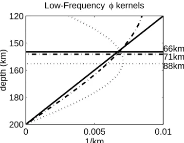
In the low-frequency limit, where the ˜φ kernel becomes a linear function of depth, the apparent depth of sampling goes to one-third the layer thickness. This value increases to half the layer thickness as the center period approaches the splitting time. Figure 6 shows three low-frequency ˜φ kernels and their apparent depths of sampling for a 200-km thick, anisotropic layer. In the low-frequency limit, the apparent depth of sampling is just 66 km whereas for data low-pass filtered at 100 mHz, the depth of sampling increases to 71 km and for data low-pass filtered at 200 mHz, it increases to 88 km.

This bias in the sensitivity to near-surface structure explains why the recovered value for ˜φ in the weak scattering case (Fig. 3b) is greater than the layer mean by about 3°. In this model, the fast axis rotates linearly from 40° at

0 0.005 0.01 200 180 160 150 120 Low-Frequency φ kernels depth (km) 1/km 66km 71km 88km

Figure 6. Low frequency Fréchet kernels and the apparent depth of sampling computed with eqn. 20. Solid line is the kernel in the frequency limit. Dashed line is the low-passed kernel for 100 mHz and the dotted line is the low-low-passed kernel at 200 mHz.

the base of the layer to 50° at the top. The kernels predict that the upper part of the model, where the fast axis ranges between 45° and 50°, will dominate the shear-wave splitting measurement and indeed, the value found numerically ( ˜φ = 48°) agrees with this prediction, corresponding to the fast axis direction approximately one-third of the way down the layer. This increase in sensitivity to the fast-axis direction near the surface may explain why shear-wave splitting measurements tend to correlate with tectonic deformation observed at the surface (Silver, 1996). Most shear-wave splitting measurements are made on seismograms with relatively low center frequencies (< 200 mHz), so that the apparent depth of sampling is less than the mean thickness of the layer. There are significant variations in the center frequencies used by different researchers, however, so this apparent depth varies from study to study.

Numerical Tests

We conducted a series of numerical experiments to test the perturbation theory derived for a homogeneous model. To investigate the sensitivity of the kernels to the reference structure, we have computed them by numerical perturbation to heterogeneous starting models. The results for starting models with a linear gradient and a step-wise discontinuity in φ(z) are compared with the homogeneous-layer case in Fig. 7. The average orientation was chosen to be the same for all three models, φ ≡ d−1

_∫

0 ( ) = 45°, while the total variation in φ(z)

was taken to be 20° for the two heterogeneous models. The kernels are very similar, indicating only a weak dependence on the starting model when the heterogeneity is of this magnitude. In particular, the apparent depths of sampling for the layered and linear model are 91 km and 90 km respectively, essentially the same as the value of 88 km calculated for the homogeneous model. The properties found for the homogeneous-layer kernels, such as their dependence on frequency, bandwidth, and incidence azimuth, should therefore pertain more generally in the weak scattering regime.

We also compared the perturbations calculated from the Fréchet kernels using eqns. (8) and (9) with the results of a direct numerical calculation that minimized the tangential-component energy on back-projected synthetic seismograms. Figure 8 shows several examples of these comparisons as a function of the average polarization direction φ for an initial pulse with a center frequency at 60 mHz and corners at 45 mHz and 75 mHz. Figure 9 plot the results for φ = 45° for increasing values of the center frequency ω₀. We note that care must be taken in the numerical calculations when evaluating the apparent splitting parameters near the azimuthal nodes at φ0 = nπ/2, because the energy

surfaces can be very flat in the ∆t' direction, and the location of the minimum is susceptible to numerical inaccuracies that can cause a π/2 ambiguity.

When the heterogeneity is small (∆φ = 10°) in the linear gradient models, the kernels do a good job of predicting ˜φ and ∆˜t for all backazimuths (Fig. 8a). For heterogeneity with a total rotation angle as large as 60° (Fig. 8b), the kernels typically overestimate the apparent splitting time by about 0.3 s, and, near the nodes, ˜φ can be off by as much as 20°. This failure of the kernels with greater heterogeneity reflects a breakdown in the small-angle approximations (e.g., eqn. B5). Inclusion of the back-scattering terms in the calculation of synthetic

0 0.005 0.01 200 150 100 50 0 K_φ (b) 1/km 35 40 45 50 55 200 150 100 50 0 depth (km) phi (deg) reference models (a) 0.01 0.005 0 0.005 0.01 200 150 100 50 0 K_∆ t (c) 1/km

Figure 7. A comparison of Fréchet kernels for three starting models. Panel (a) is a plot of φ(z) for the homogeneous-layer (solid line), constant-gradient (dotted line), and two-layer (dashed line) models. Panels (b) and (c) show the corresponding kernels for these

models, G z_φ( ) and G z_t( ), respectively. The kernels were calculated by a numerical

perturbation scheme for ω0 = 0.14 Hz, σ = ω0 /6 Hz, which are similar to the values

used in the processing of teleseismic shear waves. The models have the same average

azimuth, φ = 45°. Eqn. (10) shows that G z_t( ) = 0 for a homogeneous layer with this

initial azimuth. The agreement illustrates the weak dependence of the kernels on the starting model.

20˚ 40˚ 60˚ 80˚ 0˚ 10˚ 20˚ 30˚ 40˚ 50˚ 60˚ 70˚ 80˚ 90˚ φavg φ forwardscattering 10o _{Constant Rotation} fullscattering ~ 20˚ 40˚ 60˚ 80˚ 0 0.5 1 1.5 2 2.5 3 3.5 4 φavg ∆ t (s) ~ 0˚ 20˚ 40˚ 60˚ 80˚ 0 0.5 1 1.5 2 2.5 3 3.5 4 φavg ∆ t (s) ~ 20˚ 40˚ 60˚ 80˚ 0˚ 10˚ 20˚ 30˚ 40˚ 50˚ 60˚ 70˚ 80˚ 90˚ φavg 60o Constant Rotation φ ~ forwardscattering fullscattering 20˚ 40˚ 60˚ 80˚ 0˚ 10˚ 20˚ 30˚ 40˚ 50˚ 60˚ 70˚ 80˚ 90˚ φavg 10 Random Layers (max rotation = 30o₎

φ ~ forwardscattering fullscattering 0˚ 20˚ 40˚ 60˚ 80˚ 0 0.5 1 1.5 2 2.5 3 3.5 4 φavg ∆ t (s) ~ 0˚ 20˚ 40˚ 60˚ 80˚ 0 0.5 1 1.5 2 2.5 3 3.5 4 φavg ∆ t (s) ~ 20˚ 40˚ 60˚ 80˚ 0˚ 10˚ 20˚ 30˚ 40˚ 50˚ 60˚ 70˚ 80˚ 90˚ φavg 10 Random Layers (max rotation = 120o₎

φ ~ forwardscattering fullscattering 0˚ 20˚ 40˚ 60˚ 80˚ 0 0.5 1 1.5 2 2.5 3 3.5 4 φavg ∆ t (s) ~ 0˚ 20˚ 40˚ 60˚ 80˚ 0 0.5 1 1.5 2 2.5 3 3.5 4 φavg ∆ t (s) ~ 20˚ 40˚ 60˚ 80˚ 0˚ 10˚ 20˚ 30˚ 40˚ 50˚ 60˚ 70˚ 80˚ 90˚ φavg 10 Skewed Layers (max rotation = 120o

) φ ~ forwardscattering fullscattering 20˚ 40˚ 60˚ 80˚ 0˚ 10˚ 20˚ 30˚ 40˚ 50˚ 60˚ 70˚ 80˚ 90˚ φavg 10 Skewed Layers (max rotation = 30o

) φ ~ forwardscattering fullscattering a) b) c) d) e) f) φ ~ t ∆~

Figure 8. Comparison of numerical and analytical results. Left panels show φ˜ and right

panels show ∆˜t, plotted as a function of backazimuth. Solid lines are analytical

predictions from the kernels. Solid circles are the numerical results including back scattering and open circles include just forward scattering. a) weakly heterogeneous,

(∆φ = 10°) linear rotation model. b) strongly heterogeneous (∆φ = 60°) linear rotation

model. c) weakly heterogeneous 10 random layers model (maximum ∆φ = 30°) in which

the average fast-axis direction in the top and bottom halves are similar. d) weakly

heterogeneous 10 random layers model (maximum ∆φ = 30°) in which the layer

orientations in the top half are different than that in the bottom half. e) strongly

heterogeneous 10 random layers model (maximum ∆φ = 120°) in which the average

fast-axis direction in the top and bottom halves are similar. f) strongly heterogeneous 10

random layers model (maximum ∆φ = 120°) in which the layer orientations in the top

seismograms (solid dots in Figure 8) does not produce significantly different results from those obtained using just the forward-scattering terms.

In a second set of comparisons, we use what is perhaps a more geologically relevant model comprising 10 layers, each 20 km thick, of differing orientations constrained such that the fast-axis directions varies between 0° and 30°. When the layer orientations φi are distributed randomly, such that the average orientation in the top half of the model was similar to the bottom half, the agreement between the numerical results and the predictions of the analytical kernels is usually very good (Fig. 8c). In addition, both the exact values of the apparent splitting parameters and perturbation-theory predictions show very little dependence on the polarization angle, with the variations in the apparent splitting time associated with nodal singularities compressed into a narrow range of azimuths.

When the layer orientations are skewed, however, such that the average orientation in the top half of the model differed significantly from the bottom half (Fig. 8d), the π /2 periodicity in ∆˜t associated with the nodal singularities becomes more pronounced. This differences in the variation of ∆˜t with initial azimuth results from the fact that Gt(z) is approximately a linear function of depth that averages to zero, as seen from its low-frequency form (18). That is, the perturbation to the apparent splitting time will be small and the π /2 periodicity will be suppressed when the first moment dφ( )z z dz

0

∫

These results can be used to qualify Silver and Savage’s [1994] argument that a π /2 periodicity in initial azimuth should be diagnostic of vertical heterogeneity. This periodicity will be relatively weak for heterogeneous structures where the azimuth of the anisotropy does not vary systematically with depth.

Increasing the heterogeneity in the 10 random layers so that the fast-axis direction ranges over 120°, we find azimuthal discrepancies of up to ±5° and splitting-time discrepancies exceeding 1 s (Figs. 8e and 8f). At this level of

heterogeneity, back-scattering effects, given by the differences between the open and solid circles, begin to become important.

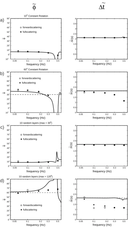
A comparison of the analytic and numerical results for different frequencies at a single backazimuth, shows that the kernels do a nice job of predicting ˜φ and ∆˜t up to 0.5 Hz when the heterogeneity is weak (Figs. 9a and 9c) but that when the heterogeneity gets stronger, the kernels break down more quickly at higher frequencies (Figs. 9b and 9d) than at lower frequencies. In these examples, ∆t =

2.14 s. At frequencies approaching 1/∆t (~0.46 Hz) the kernels predict highly

oscillatory behavior in ˜φ, which also corresponds to the frequency at which the kernels become unbounded in the single-frequency limit.

Strong-Scattering Regime

The numerical experiments demonstrate that the first-order perturbation theory expressed in eqn. (8) and (9) provides an accurate description of the apparent splitting parameters in situations where the magnitude of the vertical heterogeneity is small. As this magnitude increases, the perturbation theory fails because the small-angle approximations employed in obtaining the scattering matrix (B5) and the linearized minimization condition (B11) become inaccurate, owing to the accumulating effects of multiple forward-scattering. The combination of these strong-scattering effects causes the behavior of the apparent splitting parameters to deviate from the weak-scattering results.

Aspects of this behavior were noted in the previous discussion of Fig. 3, which display the numerical results for a constant-gradient model. In these calculations, ∆t = 2 s, φ = 45°, and all forward- and back-scattering terms were retained. For a 45° average polarization, the general form of the kernel (11) shows that the splitting-time perturbation should be zero to first order; i.e., the apparent splitting time ∆˜t should equal the total splitting strength ∆t. Strong

scattering acts to reduce ∆˜t below this theoretical limit, so that the ratio (∆t−∆t˜) /∆t, to the extent it can be accurately estimated, measures the higher-order effects. For the 30° rotation in Fig. 2c, this reduction is only about 5%, consistent with the weak-scattering approximations. The 120°rotation in Fig. 2d

0.05 0.1 0.2 0.3 0.5 0 0.5 1 1.5 2 2.5 3 3.5 4 frequency (Hz) ∆ t (s) ~ 10˚ 0˚ 10˚ 20˚ 30˚ 40˚ 50˚ 60˚ 70˚ 80˚ frequency (Hz) 10o _{Constant Rotation} forwardscattering fullscattering φ ~ 0˚ 10˚ 20˚ 30˚ 40˚ 50˚ 60˚ 70˚ 80˚ 90˚ frequency (Hz) 10 random layers (max = 30o)

forwardscattering fullscattering φ ~ 0 0.5 1 1.5 2 2.5 3 3.5 4 frequency (Hz) ∆ t (s) ~ 0 0.5 1 1.5 2 2.5 3 3.5 4 frequency (Hz) ∆ t (s) ~ 10˚ 0˚ 10˚ 20˚ 30˚ 40˚ 50˚ 60˚ 70˚ 80˚ frequency (Hz) 60o Constant Rotation forwardscattering fullscattering φ ~ 0˚ 10˚ 20˚ 30˚ 40˚ 50˚ 60˚ 70˚ 80˚ 90˚ frequency (Hz) 10 random layers (max = 120o)

forwardscattering fullscattering φ ~ a) b) c) d)

φ

~

t

∆

~

Figure 9. Comparison of numerical and analytical results. Left panels showφ˜ and

right panels show ∆˜t, plotted as a function of frequency. Solid lines are analytical

predictions from the kernels. Solid circles are the numerical results with both forward and back scattering and open circles include just forward scattering. a) weakly

heterogeneous, (∆φ = 10°) linear rotation model. b) strongly heterogeneous (∆φ =

60°) linear rotation model. c) weakly heterogeneous 10 random layers model

(maximum ∆φ = 30°). d) strongly heterogeneous 10 random layers model (maximum

gives a much more substantial effect (~35%), indicating that these approximations are not accurate for heterogeneity of this magnitude. For the 1000° rotation, the scattering is sufficiently large that the tangential-component arrivals are incoherent, so that the long-period amplitude is nearly zero, and the energy diagram looks nodal. In this case, there is no well-defined energy minimum, and it is difficult to measure the apparent splitting parameters.

In Fig. 10, we extend these calculations to constant gradient models with φ = 45°and a range of splitting and heterogeneity strengths. The ordinate is taken to be 1/κ, a quantity proportional to the inverse of the heterogeneity gradient,

0 0.5 1 1.5 2 2.5 3 0.1 0.3 1 3.2 10 32 100 strength of anisotropy, ∆t=∆s⋅d (s)

vertical correlation length, 1/

κ

, (km/deg)

small

strong, incoherent scattering weak scattering

strong, coherent scattering

0.5s 1.0s 1.5s 2.0s 2.5s 1 ° 3 ° 10 ° 30 ° 100 ° 300 ° 1000 ° anisotropy

Figure 10. Scattering Diagram Contour of split time measurements ∆˜t for smoothly

varying models. Horizontal axis shows the range of anisotropy in the models (∆t') and

vertical axis shows the range of vertical heterogeneity in the models (κ is the rotation

which defines a vertical correlation length. The contours of apparent splitting time on this plot can be used to delineate the three scattering regimes. The region with nearly vertical contours at large values of the correlation length corresponds to weak scattering, where ∆˜t ≈∆t and the perturbation theory of

Sect. 3 is valid. The deviation of these contours towards the horizontal defines a region where the scattering is too strong for perturbation theory to apply but not so strong as to prohibit the estimation of the apparent splitting parameters. The boundary between these two scattering regimes, indicated by the dashed line in Fig. 10, is given by a correlation length that increases exponentially with the anisotropy strength. As the correlation length of the vertical heterogeneity decreases at constant ∆t, the apparent splitting time decreases, at first slowly then

rapidly. Below some critical value of the correlation length (~50 km in this example, corresponding to κ = 1 deg/km), the scattering becomes so strong that

∆˜t cannot be defined.

As this diagram makes clear, it is not possible to distinguish on the basis of low-frequency splitting observations the difference between highly heterogeneous anisotropy (∆t and κ large) and weak anisotropy (∆t small).

Analysis of horizontally propagating surfaces waves (e.g., Jordan and Gaherty, 1996) is one way to distinguish between these two cases.

Discussion

For the case of weak scattering, differences in the sensitivity kernels as a function of frequency can, in principle, be exploited to invert frequency-dependent shear-wave splitting measurements for a picture of anisotropic variation with depth. To do so, one applies standard splitting analysis to broadband recordings in order to obtain an apparent fast direction to be used as a starting estimate for φ. Frequency-dependent apparent splitting parameters are then extracted by applying the back-projection procedure to narrow-band filtered seismograms, and their kernels constructed from (10) and (11). Adherence to the weak-scattering regime can be checked by confirming that minimal signal remains on the tangential-component seismogram after back-projection via the apparent splitting parameters (Fig. 4). The

frequency-dependent splitting parameters can then be inverted for φ(z). (In all of our calculations, the difference between the speeds of the two eigenwaves remained constant throughout the model. In the real world, this parameter, like the anisotropy orientation, probably varies with depth. It is a simple matter, however, to extend the theory to depth-dependent wave speeds.)

The applicability of this procedure is likely to be limited by difficulties in extracting apparent splitting parameters at higher frequencies. Above 0.1 Hz, observed shear waveforms become increasingly complex due to microseisms, crustal scattering, and other sources of "noise". In addition, split shear waves have distinct "holes" in their amplitude spectra at frequencies with integer multiples of 1/∆t (Silver and Chan, 1991), which complicate analysis at higher frequency. As a result, most shear-wave splitting analyses in the literature utilize center frequencies that fall within a relatively narrow frequency band of approximately 0.05-0.2 Hz (e.g. Silver, 1996; Fouch and Fischer, 1996; Wolfe and Solomon, 1998). Our numerical experiments in the weak-scattering regime indicate that across this bandwidth, variations in ∆˜t and ˜φ are generally less than 0.1 s and 5°, respectively (Figs. 8a, 9a). These variations are smaller than the typical error estimates in observational studies, and thus they cannot resolve changes in anisotropy with depth.

In the case of strong scattering, the approximations made in deriving the kernels are no longer valid, so that the kernels cannot be used to solve the inverse problem. We can, however, utilize the numerical results in the interpretation of splitting observations. Marson-Pidgeon and Savage (1997) report frequency-dependent shear wave splitting results from New Zealand (between 50 and 200 mHz) that are consistent with our numerical results for the strong coherent scattering regime (Figs. 9b, 9d), implying significant vertical heterogeneity with depth. In addition, splitting results from cratons in South Africa (Gao et al, 1998), Australia (Clitheroe and van der Hilst, 1998; Özalaybey and Chen, 1999), India (Chen and Özalaybey, 1998), and Tanzania (Owens et al., 1999) all find splitting times that are smaller (generally < 0.6 s) than many other continental environments (e.g. Silver, 1996). Such observations are typically interpreted as evidence for little or no anisotropy. Our calculations provide an

alternative explanation for these null results in terms of strong incoherent scattering in an upper mantle that is anisotropic, but has a high degree of vertical heterogeneity. Other data, such as horizontally propagating surface waves, are necessary to distinguish between these two possibilities.

In at least two cratonic regions where null or near-null results are reported (Australia and Southern Africa), analyses using surface waves find that the upper mantle is anisotropic between the Moho and 200-250 km depth, with ∆v_s/v_s of approximately 3-4% (Gaherty and Jordan, 1995; Saltzer et al., 1998). If perfectly aligned, such anisotropy would produce over 2 s of splitting. We interpret the apparent discrepancy between the splitting and surface-wave results as evidence for strongly heterogeneous anisotropy in these regions. In particular, both sets of observations can be explained by a model in which the local anisotropy axis remains, on average, close to horizontal, but varies in azimuth as a function of position, with a vertical correlation length on the order of 50 km (Jordan et al., 1999).

Conclusions

In both weakly and strongly heterogeneous media we find that shear-wave splitting measurements made in the low-frequency bands typically used to make observations are more sensitive to the upper portions of the model than to the lower portions. Consequently, if the orientation of the anisotropy is heterogeneous, the measured splitting direction will be more reflective of the fast-axis direction near the top of the upper mantle and the measured split time will vary as a function of backazimuth. This effect may explain why global shear-wave splitting measurements tend to correspond to the local tectonic fabric in crust beneath the observing station (Silver, 1996).

We have derived analytic expressions for sensitivity kernels that relate a perturbation in the measured splitting parameters to a perturbation in the anisotropy of the model. For weakly heterogeneous media, frequency-dependent shear-wave splitting measurements can be inverted using these kernels to determine how the anisotropy varies as a function of depth.

Variations in the strength of the anisotropy as a function of depth can be accounted for with a weighting function. Practically speaking, however, a sufficient number of measurements may not be available at high enough frequencies or with enough precision (errors are typically ±10° or more) for such an inversion to be feasible.

Strongly heterogeneous media (i.e., where the fast axis direction varies anywhere between 0° and 180°) have the additional property that they cause strong scattering. This scattering will cause the tangential component seismograms to have very little energy and a null-like energy measurement will be made despite the fact that the medium may be highly anisotropic. Our numerical experiments show that the greatest diagnostic of strong vertical heterogeneity is the drop-off in ∆˜t relative to ∆t.

Acknowledgements

Many thanks to Martha Savage, Steve Ward and an anonymous reviewer for useful comments that improved the paper. Many of the figures were generated using GMT software freely distributed by Wessel & Smith (1991). This research was funded by NSF Grant EAR-9526702.

Chapter 3

The Spatial Distribution of Garnets and Pyroxenes in Mantle Peridotites: Pressure - Temperature History of Peridotites from the Kaapvaal Craton

To be published by Oxford University Press in the Journal of Petrology by Rebecca Saltzer, Neel Chatterjee and Tim Grove, December 2001.

Abstract

We present a new method for textural analysis of mineral associations that uses digital backscattered electron and x-ray images obtained with the electron microprobe to determine the spatial properties of minerals on a two dimensional surface of the rock at different scale lengths. We determine modal amounts and average grain sizes of each mineral in the thin section without resorting to ellipsoidal approximations of grain boundaries, and investigate the spatial relationship of mineral pairs. The method is used to characterize nine mantle xenoliths erupted from kimberlite pipes in South Africa and to test whether the pyroxenes are spatially correlated with the garnets. The spatial association of these minerals is used to develop a model for the evolutionary history of the Kaapvaal peridotites. The observed distributions can be explained by a two-stage model. In stage 1, harzburgitic residues are produced by large extents of partial melting at shallow depths (~60-90 km) and high temperatures (~1300-1400° C). The melting process leading to this depletion occurs in the garnet stability field where garnet, clinopyroxene and olivine are consumed and orthopyroxene and liquid are produced. The Kaapvaal sample suite shows modal and compositional variations consistent with a progressive melt depletion event. In stage 2, the residuum is dragged down to greater depths by mantle corner flow adjacent to a subducted slab. The most depleted harzburgites descend to 140 to 160 km depth and are cooled. The least depleted harzburgites end up at shallower depths. The resulting stratigraphy is the opposite of what would be expected for a preserved mantle melt column and is consistent with inversion of the melt column as it was dragged around the wedge corner and cooled by the subducted slab. The cooling process causes clinopyroxene and garnet to exsolve from the orthopyroxene. Therefore, the depleted cratonic peridotites of the Kaapvaal preserve a temperature-pressure path consistent with an origin in an Archaean subduction zone.

Introduction

Mantle xenoliths erupted from kimberlite pipes in South Africa may provide clues to the formation and evolution of the depleted mantle that makes up the Kaapvaal craton. One hypothesis that has been proposed is that the peridotite originally resides deep in the mantle (at depths of perhaps 300 or 400 km) and is transported upwards into the cratonic lithosphere (~180 km depth), where re-equilibration occurs and clinopyroxene (cpx) unmixes from the garnet phase

[Haggerty & Sautter, 1990]. An alternative idea is that the garnet lherzolites were originally high-temperature harzburgites that originated at depths between 100 and 250 km and that both the cpx and garnet subsequently exsolved from the Al-rich orthopyroxene (opx) when the rocks cooled and re-equilibrated [Cox et al., 1987]. If exsolution of minerals has indeed occurred, then a spatial relationship between grains of minerals that were formerly dissolved in each other should be apparent in the present-day xenoliths. In particular, the first model implies a spatial relationship between cpx and garnet for rocks of pyroxenite or eclogitic compositions, whereas the second implies cpx, opx and garnet should be correlated.

The question of whether two minerals are spatially related arises frequently in petrologic studies. Despite the availability of digital images of thin sections, textural studies described in the literature are typically crystal-oriented rather than pixel-oriented [Cashman & Ferry, 1988; Kretz, 1993; Jerram et al., 1996]. These analyses generally take a "nearest neighbor approach", measuring the distance between the center of a grain and the center of its nearest neighbor, to determine whether the grains are randomly distributed, clustered, or ordered [Kretz, 1969, 1993; Carlson et al., 1995; Jerram et al., 1996; Miyake, 1998]. The most sophisticated of these involve fitting ellipsoids to a digital image of the grains, while others simply project the thin section on a screen and trace the crystals by hand. Recently, studies of digital images have used Markov-chain analysis to look for the same sort of clustering or anti-clustering of minerals [Kruse & Stünitz, 1999]. A prior spatial analysis of Kaapvaal peridotites [Cox et al., 1987] specifically tested the hypothesis that two different minerals were spatially associated and found a strong correlation between the presence of garnet and cpx with opx, but their method required labor-intensive manual outlining, identification and counting of crystals.

We describe a new technique for textural analysis in which the digital image of a thin section is statistically analyzed over a range of spatial scales. By analyzing the pixel data, we determine the modal amounts and average crystal size for each mineral type and examine whether any of the minerals are more closely associated spatially than would be expected if they were randomly

distributed. This method may be applicable to different textural studies in which average crystal sizes need to be determined or the relationship between mineral types, and in particular their spatial relation due to metamorphism or metasomatism, needs to be assessed. We apply this statistical method to nine mantle xenoliths erupted from kimberlite pipes in South Africa to determine which, if any, of the constituent minerals are correlated. In this way, we test the two hypotheses regarding the history of South African mantle xenoliths and, by implication, the structure and evolution of the Kaapvaal craton.

Sample Selection

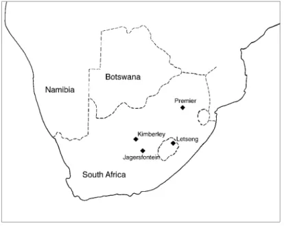
We selected three garnet-peridotite xenoliths from the Bulfontein kimberlite pipes (Kimberley, South Africa), four from the Jagersfontein pipes (130 km SSE of Kimberley), one from the Premier Pipes (25 Km NE of Pretoria, South Africa) and one from the Letseng pipes in northern Lesotho (Fig. 1).

Figure 1. Map of southern Africa. Nine, low-temperature, garnet-peridotite xenoliths were collected from the four kimberlite pipes shown.

Several criteria were applied in selecting the sample suite. All samples contained dominantly olivine and opx with the coarse texture that characterizes low-temperature peridotites [Boyd, 1987]. Peridotite nodules (~25 × 25 × 10 cm) were

cut into multiple slabs (3 to 5 slabs each ~1cm thick) and samples were chosen from nodules that had a uniform distribution of garnet and cpx in all slabs. Samples that contained clots of garnet and cpx were avoided, as were samples that contained veins of phlogopite or samples that were serpentinized. We also avoided samples that appeared to have undergone metasomatic modification. A suite of representative low-temperature peridotites that spanned the range of modal olivine percentages observed by Boyd [1989] were supplied by F.R. Boyd.

Mineral compositions and modal analysis

From each slab we prepared two by three inch polished thin sections for chemical and modal analysis. We obtained a back-scattered electron image (brightness corresponding to atomic number) as well as x-ray concentration maps of Si, Al, Ca, and Mg) of each thin section using the four wavelength dispersive spectrometer-JEOL JXA-733 Superprobe electron microprobe at MIT. We used an accelerating voltage of 15 kV, a beam current of 100 nA and a dwell time of 5 ms per spot. By comparing the various images, we were able to identify each pixel in the image as either olivine, orthopyroxene, clinopyroxene or garnet. Eight of the samples we mapped and analyzed are shown at the same scale in Fig. 2. The image resolution ranged between 62 microns/pixel to 200 microns/pixel and the areas imaged were approximately 3 cm × 5 cm. Depending on the image resolution and the area mapped, the image collection time varied between 12 to 16 hours per sample.

Chemical Compositions

Chemical compositions of the minerals were obtained for five of the samples with the same electron microprobe at MIT using wavelength dispersive spectrometry. Phases were analyzed at an accelerating voltage of 15kV, a beam current of 10nA, a beam diameter of ~1 micron and typical counting times between 20 and 40 seconds per element. Data were reduced with the CITZAF program [Armstrong, 1995] using the atomic number correction of Duncumb and Reed, Heinrich’s tabulation of mass absorption coefficients and the fluorescence correction of Reed. A minimum of 10 measurements were made for each