Distributed communication network wireless siting and propagation studies

Distributed Communication Network Wireless

Siting and Propagation Studies

by

Win Chevapravatdumrong

SUBMITTED TO THE DEPARTMENT OF ELECTRICAL ENGINEERING AND

COMPUTER SCIENCE IN PARTIAL FULFILLMENT OF THE REQUIREMENTS FOR THE

DEGREE OF

MASTER OF ENGINEERING IN ELECTRICAL ENGINEERING AT THE

MASSACHUSETTS INSTITUTE OF TECHNOLOGY

May 2001

I- v

©D 2001 Win Chevapravatdumrong. All ri ghts reserved.

BARKER

The author hereby grants to MIT permission to reproduce and to distribute publicly paper and electronic copies of this thesis document in whole or in part and to grant others the

right to do so.

Author

De arment of Electrical Engineering and Computer Science

Certified by

Michael A. Deaett Charles Stark Draper Laboratory Thesis Supervisor

Certified by_

Prof D vid H. Staelin

T hesli Advisor

Accepted by_

Prof. Arthur C. Smith Chairman, Department Committee on Graduate Theses

MASSACHUSETTS INSTITUTE OF TECHNOLOGY

JUL 1 1 2001

Distributed Communication Network Wireless

Siting and Propagation Studies

by

Win Chevapravatdumrong

SUBMITTED TO THE DEPARTMENT OF ELECTRICAL ENGINEERING AND COMPUTER SCIENCE ON MAY 18, 2001 IN PARTIAL FULFILLMENT OF THE

REQUIREMENTS FOR THE DEGREE OF

MASTER OF ENGINEERING IN ELECTRICAL ENGINEERING

AT THE

MASSACHUSETTS INSTITUTE OF TECHNOLOGY

Abstract

This thesis analyzes siting and propagation studies for a real-time unmanned aircraft navigation system and other wireless distributed control systems where the type of terrain will often be unknown. Field measurements were made of the 2.4-GHz propagation characteristics for a variety of abnormal siting situations and realistic field environments in which the systems will be deployed. The mobile test equipment consists of two small, programmable transceivers that can measure received signal strength. This equipment is programmed to facilitate automated measurements as described in the thesis. Propagation characteristics were investigated using a structured framework that divides measurements into large-scale deterministic, small-scale statistical, and large-scale statistical analysis.

Empirical data from several environments and siting situations for both large-scale and small-scale fading were collected. The large-small-scale deterministic measurements verified the 2-ray model and yielded a path loss exponent of d2 2 8 _{in simple network configurations, where d is distance in}

meters, as well as a loss of d-3 87 _{in the Vvedensky region. The small-scale statistical}

investigations verified a close fit to Ricean-distributed multipath fading with a line-of-site path. Small-scale measurements also revealed significant changes (up to 15 dB) in propagation due to minor spatial antenna movements, as well as Doppler spread values ranging from 0.5 to 2.5 Hz. Large-scale statistical investigations determined path loss exponents for various environments over distances of up to 150 meters. These values ranged from 2.11-3.18 in urban environments to almost 4 in environments with thick vegetation.

Communication system design implications based on these results are discussed. The small-scale findings demonstrate that link level spatial redundancy is required to provide adequate network performance. The large-scale findings provide realistic distance-dependent loss data necessary for calculating network link budgets.

Faculty Thesis Supervisor: Prof. David H. Staelin Draper Thesis Supervisor: Michael A. Deaett

Acknowledgments

I first and foremost would like to thank the Charles Stark Draper laboratory for

sponsoring my research on this project. I would also like to thank my Draper advisor, Michael Deaett, for his endless technical guidance and support, as well as his help in

conducting field measurements in any and all types of weather conditions. Also, I would

like to thank Professor David Staelin, my MIT faculty thesis advisor, for his technical

assistance and direction. Additionally, I would like to thank Robert Tingley and Vincent

Attenasio from the Draper RF and Communications Group for their patience and

technical help, as well as numerous other Draper employees for their support and

guidance: Pat Callinan, Seth Davis, Stephen Finberg, Michael Aiken, John Ford, and

Valerie Lowe. Finally, I would like to thank my family-Wichai, Suwannee, and Cherry

Chevapravatdumrong-whose endless encouragement provided the motivation for the

ACKNOWLEDGMENT

May 18, 2001

This thesis was prepared at The Charles Stark Draper Laboratory, Inc., under project 13046-Distributed Data Link Network Design.

Publication of this thesis does not constitute approval by Draper or the sponsoring agency of the findings or conclusions contained herein. It is published for the exchange and stimulation of ideas.

Table of Contents

1

1.1 Past Work ... 12

1.2 Problem Description ... 13

1.3 Thesis Outline and Approach ... 13

2 Propagation M odeling Theory... 15

2.1 Large-Scale Fading ... 17

2.1.1 Large-Scale Statistical Analysis ... 17

2.1.2 Large-Scale Deterministic Analysis: 2-ray Model ... 20

2.2 Small-Scale Fading ... 24

2.2.1 Distribution of Path Amplitudes ... 24

2.2.2 Parameters of Small-Scale Multipath Fading ... 26

3 Measurement System Overview ... 29

3.1 Commercial Hardware ... 30

3.2 Internal Draper Hardware: DWN Transceiver ... 31

3.3 DWN Transceiver Design ... 33

3.4 Software Design ... 35

3.4.1 Transmitter ... 35

3.4.2 Receiver ... 37

3.5 Packaging ... 40

4 Test Suite Design and Characterization ... 43

4.1 RSSI Characterization ... 44

4.2 Antenna Characterization ... 47

4.2.1 Antenna Resonance ... 48

4.2.2 Antenna Gain ... 48

4.3 Sampling Rate and Test Duration ... 50

4.4 Test Suite Summary ... 51

5 Large-Scale Deterministic Modeling: 2-ray Model ... 53

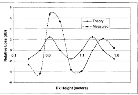
5.1 Attenuation Function Height Dependency ... 54

5.2 Attenuation Function Distance Dependency ... 57

5.3 Vvedensky Region ... 60

5.4 Deterministic Large-Scale Path Loss Model ... 61

6 Small-Scale Statistical Modeling ... 63

6.1 Small-Scale Amplitude Distributions ... 64

6.2 Coherence Time and Doppler Spread ... 69

6.3 Small-Scale Fading System Design Implications ... 72

7 Large-Scale Statistical Modeling ... 75

7.2 Urban Setting ... 78

7.3 Single Tree Propagation ... 80

7.4 Summary of Large-Scale Results ... 81

7.5 Large-Scale Fading System Design Implications ... 81

8 Conclusion ... 83

A Additional Measurements ... 87

B Maps and Photographs ... 92

C Hardware Overview Chart ... 99

D Antenna Datasheets ... 101

List of Figures

2-1 Configuration for 2-ray Reflection Model ... 20

2-2 Method of images geometry ... 23

3-1 Block diagram of DWN Transceiver in transmit mode ... 33

3-2 Block diagram of DWN Transceiver in receive mode ... 34

3-3 Toko antennas ... 34

3-4 Receiver information flow ... 37

3-5 Receiver instrument setup ... 41

4-1 RSSI calibration curves ... 45

4-2 RSSI rise time ... 46

4-3 RSSI fall tim e ... 46

4-4 Generic field test configuration ... 47

4-5 Toko antenna gain characterization setup ... 49

5-1 2-ray height dependency measurement setup ... 55

5-2 Measured and theoretical values of path loss about a mean vs. receiver height. 56 5-3 General case of attenuation function ... 57

5-4 Briggs field calculated attenuation function vs. separation distance ... 59

5-5 Briggs field measured and theoretical values for path loss vs. separation distance ... 59

5-6 Measured values for path loss vs. separation distance in Vvedensky region ... 61

5-7 Measured F region and Vvedensky region path loss vs. distance ... 62

6-1 Photographs of multipath fading measurement locations ... 65

6-2 Histograms of small-scale amplitude measurements ... 66

6-3 Path loss vs. horizontal distance for small-scale experiments ... 67

6-4 Time-domain and Fourier Transform Doppler spread plots ... 70

7-1 Path loss vs. distance at Alewife Preserve ... 76

7-2 Example measured values for large-scale distribution at Alewife Preserve .... 77

7-3 Path loss vs. distance along Vassar Street ... 79

A-1 Transmitter siting locations atop parking garage ... 88

A-2 Photographs of transmitter atop parking garage ... 88

A-3 Diagram of corner measurements ... 89

A-4 Photograph of corner measurements ... 90

B-1 Diagram of Alewife Preserve measurements ... 92

B-2 DWN transmitter 1 meter high above low-lying vegetation ... 93

B-3 DWN transmitter amongst low-lying vegetation ... 93

B-4 Diagram of measurements conducted along Vassar Street ... 94

B-5 Photograph of Vassar Street ... 95

B-6 Map of Vassar Street ... 95

B-7 Additional map of Vassar Street ... 96

B-8 Diagram of Thorndike Park measurements ... 97

List of Tables

3-1 DW N Transceiver specifications ... 32

3-2 SCI register descriptions ... 36

3-3 ATD register descriptions ... 38

4-1 Summary of Toko gains ... 50

4-2 Hardware and test suite summary ... 51

6-1 Summary of Doppler spread and coherence time measurements ... 71

7-1 Summary of large-scale results ... 81

A-1 Theoretical distribution parameters for measurements from section 6.1 ... 91

C-i Hardware overview ... 99

Chapter 1

Introduction

Physical layer transmission capability is the foundation of any communication or radar

system; without transmission across a given media, no information can be sent. This

transmission capability for wireless systems is highly dependent upon two factors: siting

and propagation. Siting refers to placing a communication device in an environment so

that it can radiate from its immediate surroundings. Having sited two devices,

propagation refers to the ability to transmit energy directly from one device to the other

in that given environment.

The purpose of this project is to perform siting and propagation studies for a real-time

unmanned aircraft navigation system and other distributed control systems employing

wireless connectivity. The navigation system acts as a wireless network with Grid Relay

Stations (GRS units) that transmit updated location and destination coordinates to

in-flight aerial users. The system is designed as a pre-planned network, meaning it is

results of this project's studies are useful in the performance prediction phase of network

planning.

One important feature that differentiates the navigation system from other wireless

navigation systems is its method of deployment. The GRS units are arranged or simply

dropped in the local area between the source and destination sites. While such an ad-hoc

network offers flexibility in topology and host distribution, it should be noted that the

type of terrain in which the system is deployed will often be unknown. For this reason, it

is necessary to conduct propagation studies in different environments and topologies in

order to simulate possible deployment configurations.

1.1

Past Work

Extensive work has been performed in the realm of propagation modeling. Demand for

such studies is due mostly to the worldwide rollout of cellular mobile communication

systems and wireless LANs. Indoor radio propagation modeling work can be found in

[1-4]. Outdoor studies for cellular systems have also been performed [5-10]. These

studies are all helpful in understanding various methods and waveforms used for

propagation modeling. Such work is often based on commonly used mathematical and

statistical models. Some of these models include the Longley-Rice, Hata, and Okumura

models [11-13].

Since most published propagation work has been tailored specifically for cellular

applications, findings are not applicable to the navigation system. In cellular applications

and models, larger communication distances and tall base stations are assumed. For

a few studies that explore the type of configurations required by the navigation system

[14-15].

1.2

Problem Description

As such, there is clearly a need for further studies more specific to the requirements of

the navigation system. This project will focus on two primary issues of concern:

propagation characteristics of radio frequency (RF) waves through a variety of

environments, as well as siting methods for the distributed wireless components (GRS

units) of the system. Measurement hardware must be developed that is capable not only

of performing the necessary tests, but also of enabling mobility of the test equipment.

1.3

Thesis Outline and Approach

Chapter 2 begins with explanations of the manner in which propagation modeling was

performed. A framework is introduced around which the measurements were based. An

overview of theory for both large-scale and small-scale modeling is offered, as well as a

discussion detailing the difference between deterministic and statistical modeling.

Equations are developed that serve as foundations for the propagation measurements.

Next, Chapter 3 is an overview of the hardware selection process and reasons for why

the DWN transceiver was selected as the measurement system. Discussion then moves to

the topic of the transceiver itself-how it is designed, how it functions, etc. Design of the

entire measurement system will then be reviewed, including software design, hardware

Chapter 4 is an explanation of how the propagation measurements were actually

performed. It reviews how the hardware was characterized, as well as how results of the

measurement system can be used for propagation modeling. A test suite summary is

discussed, detailing the manner in which each measurement is made.

Chapter 5 is the first chapter presenting results from propagation measurements. It

discusses data gathered from large-scale deterministic experiments and formulates a

model for low-ground communication in open environments. More theory about the

2-ray model beyond what is discussed in Chapter 2 is presented.

Chapters 6 and 7 contain the more comprehensive statistical propagation studies.

Small-scale measurements are discussed in Chapter 6 and results are analyzed. Chapter 7

offers similar content, but overviews the large-scale measurements.

Finally, Chapter 8 summarizes the project and discusses the importance of the work

towards what is needed by the navigation system for network design. Possibilities for

Chapter 2

Propagation Modeling Theory

There are many complex mechanisms that govern radio propagation, and in a wireless

ad-hoc communication system, these mechanisms vary vastly across different environments.

Mechanisms that govern radio wave propagation are often separated into three different

contributing phenomena: reflection, diffraction and scattering [11].

* Reflection. Reflection occurs when a radio wave bounces off of a flat surface

whose dimensions are much larger than the wavelength of the propagating wave.

* Diffraction. Diffraction occurs when there is a large impenetrable body between

transmitter and receiver. Secondary waves essentially "bend" behind the object,

causing signal reception at the receiver even without line-of-sight (LOS).

* Scattering. Scattering is due to the existence of objects small compared to the

wavelength of the propagating wave. Energy is re-radiated by these objects,

When these three phenomena work in conjunction to alter a signal, numerous paths of

different strengths, phases, and arrival times may arise, making a received signal very

unpredictable.

Propagation modeling measurements seek to provide either a deterministic analysis of

these mechanisms or a statistical model detailing on average how these mechanisms will

behave. Deterministic analysis involves using physics and simple analysis of radio wave

propagation to accurately predict and explain the results of field measurements.

Statistical modeling is in essence a reverse process, where statistics of channel

parameters are derived based on these measurements.

This project seeks to mitigate the unpredictability of radio wave propagation in

wireless ad-hoc communication systems by using a framework containing both

deterministic analysis as well as statistical modeling. The framework is built around the

idea that propagation characteristics of wireless channels can be analyzed using two

different classes of fading effects: large-scale and small-scale.

Large-scale fading refers to average signal power attenuation or path loss due to

distance variations. It also refers to attenuation variations exhibited when a channel's

physical structure changes significantly for local areas with the same antenna separation

but different transmitter/receiver geometry. Large-scale fading is generally affected by

reflection or diffraction off of large objects [19]. Small-scale fading refers to signal

strength fluctuations over a short period of time or distance due to multiple scatterers.

Generally in most outdoor environments, a received signal is affected by a

combination of the two phenomena. This signal is often modeled as a small-scale

Understanding both phenomena-and being able to separate their contributions to overall

signal fluctuation-is important to the design specifications of radio communication

systems.

2.1

Large-Scale Fading

Large-scale fading can be examined from the perspective of either deterministic analysis

or statistical modeling. The application of one or the other approach is dependent upon a

given outdoor setting. In a complex setting with numerous obstructions, a signal will

experience unpredictable phase and amplitude fluctuations. Because of the difficulty in

deterministically quantifying such alterations to the signal, a more realistic approach to

modeling these situations is to perform statistical analysis based on field measurements.

In settings with minimal obstructions, radio wave propagation can be reduced to simple

models based on reflection. In such cases, a physics-based deterministic approach is used

[16]. This project will investigate large-scale fading phenomenon using both techniques.

2.1.1

Large-Scale Statistical Analysis

In large-scale studies, one purpose of field measurements is to provide a way of

calculating path loss as a function of distance. Such information is essential in

determining the size of the coverage area for a radio communication system in any

environment, as well as understanding optimum antenna deployment locations [4]. This

path loss can be expressed as attenuation of received power in terms of transmitted

power. Ideal radio wave propagation assumes that a signal is sent between transmitter

contribute significantly to path loss, and therefore free space is an inaccurate

representation of the propagation that actually occurs. Statistics of path parameters must

be determined in order to estimate the performance of a signal across any non-ideal

wireless channel exhibiting such behavior.

Large-scale fading statistics with respect to this path loss refer to calculating a mean

path loss, as well as a variation about this mean [17]. Path loss can also be viewed in

terms of an nth-power law-the mean received signal power fades exponentially (to the

nth power) as a function of distance from a transmitter [18].

The large-scale statistical analysis and measurements to be made will be based on the

path-loss exponent model. In order to clearly understand how and why this model

describes a wireless channel, it is important to view its derivation based on the physics of

radio wave propagation.

The Friis equation is a simplified model of radio wave propagation in a single-path

free space channel. It expresses the level of received power Pr in terms of transmitted

power P. In free space, this relationship is given by:

2

Pr

_

= GtGr (2.1)

where Gt and Gr are the respective gains of the transmitter and receiver antennas, A is the

signal wavelength, and d is the antenna separation distance. If we define

P = PGrG,(A/4;zdo)2 _{as the received power at a reference distance do, then we can}

reduce Equation 2.1 to:

I 2(2.2)=o d2

As previously mentioned, path loss can be viewed in terms of an nth power law where

received signal power fades exponentially (to the nth power) as a function of distance

from a transmitter. In free-space, the value of n-the path-loss exponent or

distance-power gradient-is 2. However, in non-ideal environments, this value usually ranges

anywhere from 2 to 6. Therefore, extending Equation 2.2 to a non-ideal environment

where obstructions are present, the received signal power Pr can be expressed as a

function of distance d between transmitter and receiver:

P= d (2.3)

This distance-power relationship can be also expressed in decibels (dB) as:

10 logOP, = 10loglo P -10nlogjo(d/ do) (2.4)

If we define the path loss in decibels at a distance of do as LO= 10logioPt-10logioPo [16],

the path loss Lp in dB for an environment with a loss exponent n can be expressed as:

L, = Lo +10nlog 10(d / do) (2.5)

Equation 2.5 is the definition of path-loss found in [11, 16-18].

This distance-power relationship only represents a mean value, though, and in order

to create an adequate large-scale path loss model for an arbitrary wireless channel, it is

necessary to provide for statistical variations about this mean due to changes in the

environment. This variation is often modeled in [17] as a random variable with a

log-normal distribution (see section 7.1). Taking this into consideration, we arrive at the

path-loss exponent model:

L, = Lo +1Onlog10 (d / do) + X, (2.6)

hI

hr

Distance d

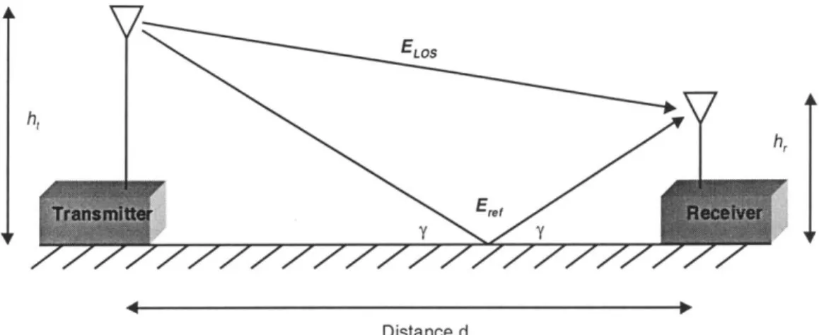
Figure 2-1: Configuration for 2-ray reflection model.

2.1.2

Large-Scale Deterministic Analysis: 2-ray Model

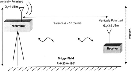
In simpler network configurations where obstructions between transmitter and receiver

are limited, it is possible to use a deterministic physics-based approach to propagation

modeling. Figure 2-1 shows the necessary configuration in which such an approach

applies. It is clear that radio transmission in a simplified configuration can be treated as

the sum of a line-of-sight ray and a ground-reflected ray. The appearance of this second

ray alters the E-field at the receiver, and thus the Friis free-space propagation given in

Equation 2.1 is inaccurate. Dolukhanov [19] redefines propagation taking into account

this reflected ray and includes in his model an attenuation function F where free-space

propagation loss can now be defined as:

2

Pr AF

- =GtGr( (2.7)

F in Equation 2.7 is dependent upon the geometry of the network configuration, as well

as the surface off of which the radio wave is reflected.

The free-space rms and peak strengths of an E-field in mV/m at a receiver are given in [19] by: Eri, = 173 JPG1 (2.8) d VPGI Epeak = 245 d (2.9)

where P, is the output power of a transmitter in kW, G, is the transmitter antenna gain,

and d is the distance between transmitter and receiver in km. Accounting for the

attenuation function F, Dolukhanov defines the altered E-field as:

J G1

ErmsF 173 F (2.10)

From 2.1.1, reflection occurs when a radio wave bounces off of a flat surface whose

dimensions are much larger than the wavelength of the propagating wave. Reflection of

a radio wave from an imperfect conductor (i.e. the earth's surface) changes both the

amplitude and phase of the wave. This change can be described in terms of a complex

reflection coefficient R = Re-i where R yields the change in amplitude and 0 the change

in phase. To find the values of R and 0 for a surface, [19-21] can be used. First, the

dielectric constant F and conductivity c; of the surface must be known. These values for

various surfaces can be found in Chapter 2 of [19]. Using these values, charts from

[20-21] can be used to estimate R and 0.

Based on radio wave reflection theory, the peak E-fields in mV/m for the LOS and

reflected rays in Figure 2-1 are given by:

Ee = R*245 e (2.12)

ref d±Ad

where w is the phase in radians of the original ray and R and 0 are the amplitude and

phase of the complex reflection coefficient of the reflector. Ad is the difference in path

length between the LOS ray and the reflected ray. Since Ad << d in all practical cases,

the total peak E-field at the receiver in Figure 2-1 is defined by Dolukhanov in [19] as:

SPG

Etota =ELOS + re = 245 d l[1+ Re-J]e" (2.13)

where

B

received field:

Etotans =173 V ]1+2Rcos(o + 2g Ar)+R2 (2.14)

Comparing Equation 2.14 with Dolukhanov's equation for the altered received E,,ns field,

it is clear that the attenuation function F can be defined as:

F= 1+2Rcos(6+ 21Ad)+ R2 (2.15)

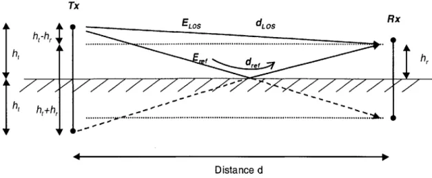
The method of images [11] in Figure 2-2 can be used to find the value of the path-length

difference Ad in Equation 2.15. The lengths of the LOS ray dLos and the reflected ray dref

in meters are: h,2 - 2hh, +hr 2 dLOS = (h, -h) 2 +d 2 =d + 2d (2.16) dre = V(h, + hr )2 +d 2 ~ d + h2 _{+ d (2.17)} 2d (.7

where h, and h, are the transmitter and receiver heights in meters and d is the antenna

Rx . ELOS dL OS hr

777

77

7$I~7>7 .7777.~772771277

Figure 2-2: Method of images geometry.

Since Ad is simply defined as dref - dwos, subtracting Equation 2.16 from 2.17 gives (in

meters):

Ad = dref -d LOS 2h hr

LOS (2.18)

As such, the attenuation function F can be redefined as:

F= 1+2Rcos(O+ 'd )+R 2 (2.19)

Assuming perfect ground reflection (R=1) and a small grazing angle (0=180), Equation

2.19 can be simplified even further:

F=2sin-Ad = 2 sin

A A (2.20)

Under these perfect assumptions, Dolukhanov [19] states that the received E-field can

then be defined as the free-space E-field multiplied by F in Equation 2.20.

definition is also found in the classic 2-ray model derived by Rappaport in [11].

This Tx L A ht-hr I A h+hr I I I

2.2

Small-Scale Fading

Unlike its large-scale counterpart, small-scale fading is not dependent so much on

reflection and diffraction as it is on the mechanism of scattering. Scattering causes an

effect of having two or more versions of the transmitter signal arrive at the receiver at

slightly different times. This phenomenon, called multipath fading, can lead to a received

signal that varies widely in amplitude and phase with small changes in time or travel

distance [11].

2.2.1

Distribution of Path Amplitudes

Understanding received signal strength fluctuations across small travel distances or time

intervals is crucial in small-scale fading analysis. The transmit power of an ad-hoc

communication system can be designed to accommodate such fading. In a multipath

environment, numerous distributions have been used to describe the small-scale fading

envelope. The type of distribution often depends on environment, as well as the absence

or presence of a dominating LOS component [4].

Rayleigh Distribution

Clarke [23] first used the Rayleigh distribution to model a mobile channel multipath

fading envelope in absence of a strong line-of-sight component. The probability density

function of the distribution is given by:

r Fr2

where the mean, variance, and median are defined as o-71/2, a2(2-z/2), and 1.177a,

respectively. Theoretical explanations of the applicability of the Rayleigh distribution to

multipath environments can be found in [4] and [22].

Ricean Distribution

The Ricean distribution is said to occur when a strong LOS or dominant signal

component exists between transmitter and receiver. The received signal then consists of

the multipath Rayleigh vector, as well as a vector deterministic in amplitude and phase,

representing the LOS path. The pdf of the distribution is given by:

r r2 +v2 rv

Pr(r) -- exp - 2 (2.22)

where Io is the zeroth-order modified Bessel function of the first kind, v is the magnitude

of the dominant component, and a2 is the variance of the multipath. The Ricean

distribution is often described in terms of the Ricean factor K, defined as K = A2 /2U.

Further discussion of the theoretical relationship between this distribution and LOS

multipath fading can be found in [4] and [11].

Log-normal Distribution

This distribution, as discussed in Section 2.1.1, is often used to describe large-scale

variations of signal amplitudes in a given environment. The pdf is given by:

1

{(1nr

-p)2]

Pr(r)= exp - 2 (2.23)

In this distribution, log r is normally distributed with mean p and standard deviation a.

Theoretical explanations for this distribution in large-scale fading can be found in [4] and

[23].

2.2.2

Parameters of Small-Scale Multipath Fading

The scattering of small-scale fading is caused by two mechanisms [11, 17]:

1) Time-dispersion resulting from the characteristics of the fading channel's impulse

response.

2) Time-variance resulting from slight antenna movement or spatial changes in the

local environment

Bello [24] first introduced a way to model such fading phenomenon by treating the

mobile channel as exhibiting wide-sense stationary uncorrelated scattering (WSSUS).

More specifically, the WSSUS channel is wide-sense stationary in both time and

frequency domains and also exhibits uncorrelated multipath scattering at the receiver

[24]. This model can be used to describe the time-dispersive and time-variant nature of

the multipath channel [11, 17, 24].

Time Dispersion: Delay Spread and Coherence Bandwidth

The multipath intensity profile is a function defined by Bello [24] that plots a channel's

received power impulse response versus time delay r [17] in seconds. The maximum

excess delay is defined as the time delay during which multipath signal power falls a

certain threshold below the maximum value [11, 17]. A mean excess delay and rms

excess delay Y is the first moment and rms delay spread a- is the square-root of the

second central moment of the multipath intensity profile [4].

Coherence bandwidth B, (Hz) is a statistical measure of the frequency bandwidth

over which the channel passes all spectral components with approximately equal gain and

linear phase [11, 17]. Several different sources define BC in terms of rms delay spread,

though these sources vary in the exact mathematical relationship between the two

parameters [17]. In [11], BC is defined as the bandwidth where the frequency correlation

function exceeds 0.5, so BC ~ 1/5a- .

Time-Variance: Coherence Time and Doppler Spread

Time-variance in a channel is caused by slight motion of or between the transmitter and

receiver in the ad-hoc communication system. It is well known that such motion causes

the received frequency to be shifted relative to the transmitted frequency. This shifting, the Doppler frequency shift, fd, is given as [16]:

fd = fc (2.24)

where v,,, is the speed of motion of or between transmitter and receiver and

f,

Doppler shift, or the bandwidth fromfe -fd tof, +fd _{in the Doppler power spectrum D(X),}

a plot of magnitude versus frequency that represents the strength of shifts at different

frequencies. A more specific measure of Doppler spread, the rms Doppler spread (Hz), is

A2D(A)dA

BD J(2d= (2.25)

fD( A)d A

Coherence time Tc (seconds) is a statistical measure of the time duration over which

the channel impulse response is invariant [11]. The approximate relationship between

Doppler spread and coherence time is given by [11, 17]:

1

T = BD-rms2.26)

This chapter developed a framework around which to perform propagation measurements

based upon large-scale and small-scale fading theory. Based on this framework,

experiments were designed for the field measurements. The next step was to build

Chapter 3

Measurement System Overview

While many past propagation modeling efforts have been performed using large,

immobile equipment such as network analyzers, the emphasis on this study was to

provide not only capable measurement hardware, but also equipment that would mimic

the siting methods of mobile networks. Therefore, while investigating hardware options

for the study, two primary questions were raised:

1) What is the measurement capability of the hardware?

2) What is the siting flexibility of this unit?

Previous discussions have reviewed the two different types of fading classes to be

studied: large-scale and small-scale. Knowledge of both phenomena is critical when

designing a communication system to function across a wireless channel. The former

question addresses this need. In designing the propagation modeling hardware, finding

equipment with the capability to perform such measurements was essential. The latter

question involves examining the size of the hardware and how the hardware can be

equipment should consist of both a mobile transmitter and receiver, i.e. no large

analyzers. The hardware can then be deployed into any abnormal network configuration.

3.1

Commercial Hardware

While the emphasis on this study was to perform propagation modeling experiments, a

secondary effort was dedicated to developing or altering hardware for these

measurements. Additionally, upgrade capability of the hardware to a data

communication network was considered. As such, initial hardware investigations

focused on examining readily available commercial products with network

communication capability (see Appendix C). Chipsets for two established wireless

protocols-802. 11 wireless LAN and Bluetooth-were considered, but proved not to be

the strongest candidates for measurement purposes.

Intersil Corporation is the producer of the Prism II chipset, an 802.11

WLAN-compliant chipset that transmits up to 11 Megabits/second using Direct Sequence Spread

Spectrum (DSSS) signaling in the ISM band. Intersil manufactures and sells evaluation

boards packaged as PCMCIA cards for laptop computers, allowing a certain level of

mobility. However, while these boards function perfectly as communication units,

altering them for propagation experiments seemed beyond the schedule and scope of the

project. Bluetooth, which uses Frequency Hopped Spread Spectrum at data rates up to 1

Mbit/s, was also considered. Many companies including Ericsson and National

Semiconductor offer chipsets. However, a similar problem as the Prism II exists in that it

is difficult to alter the hardware and software of the evaluation boards for propagation

There are also many commercial spread spectrum transceivers on the market that

were considered for the studies. Xetron Corporation sells the Hummingbird 900 MHz

spread spectrum transceiver and Linx Technologies sells the Linx. While both of these

transmitters provide spread spectrum communication, wideband measurements would

require a spectrum analyzer on the receiver, thereby limiting the necessary siting mobility

previously discussed.

3.2

Internal Draper Hardware: DWN Transceiver

Because of the lack of mobility or measurement capabilities in commercial hardware, the

investigation into measurement equipment became focused on internal Draper hardware.

The Draper Wireless Network (DWN) transceiver is a small, programmable unit that

sends continuous wave (CW) or binary frequency-shift keying (FSK) modulated

waveforms across an approximately 100 MHz bandwidth in the ISM band. It was

originally designed as a data transceiver for a wireless local shipboard network that was

used for communication between remote sensors and several access points.

The DWN transceiver seemed to be the optimal solution in the hardware investigation

for numerous reasons:

1) Measurement flexibility. With an on-board microprocessor, the transceiver

can be programmed to any carrier frequency within its bandwidth.

Additionally, any binary data stream can be transmitted. In receiver mode, the

2) Siting flexibility. The compactness of the transceiver (it measures -2.5" by

3.5") renders it extremely mobile. It can therefore be placed in various

configurations and locations.

3) Primary Draper information sources. The DWN transceiver was fully

designed internally by communication systems and RF engineers at Draper

Laboratory. Therefore, any questions of usage or alterations can be directed

first-hand to the designers of the board.

4) Upgrade capability. As previously mentioned, a secondary goal of the project

was to find hardware that could be utilized not only as a measuring/modeling

system, but that could be upgraded to a mobile data communication network.

The DWN transceiver has such capability.

For these reasons, the transceiver was selected as the primary hardware centerpiece of the

propagation modeling equipment. Design specifications for the DWN board can be

found in Table 3-1.

Data Rate 57.6 kilobits/second

Center Frequency 2.45 GHz

Bandwidth 195 MHz (2290 - 2485 MHz)

Number of channels across bandwidth 140 channels

Modulation Type fo +/- 50 kHz Binary FSK or CW

Synthesizer Frequency Hop Time < 1.0 millisecond

Transmit Power Level - 1 milliwatt (mW)

Antenna Polarization Vertical

Voltage 3.3 Volts

3.3

DWN Transceiver Design

The DWN transceiver consists of two primary sections: the microprocessor and the radio

unit, both on a single board. The programmability of the transceiver is derived from the

microprocessor section. It contains a Motorola 68HC12A4 microprocessor, a 16-bit

8-MHz microprocessor with various on-chip peripheral modules, including two serial

communication interfaces, an 8-bit analog-to-digital converter, 1024 bytes of RAM, and a

4 Kbyte EPROM. The ease of usage of the HC12, along with its peripherals, renders the

transceiver an excellent measurement system for propagation modeling.

The other side of the transceiver board contains the radio section. This functions both

as a transmitter and receiver, depending on how the microprocessor is programmed.

Various control signals from the HC12 determine the functionality of the radio section.

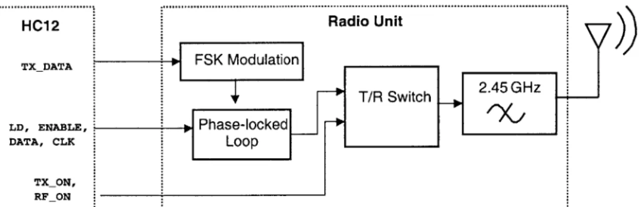
Figures 3-1 and 3-2 are block diagrams detailing transceiver functionality in transmit and

receive modes, respectively. Both figures show the essential control signals from the

HC 12 needed for proper radio functionality.

Radio Unit TXDATA sFSK Modulation T/R Switch 24 ~ LD, ENABLE, Phase-locked -DATA, CLK Loop TX ON, RFON

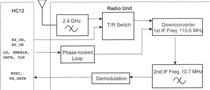
... .... .. ... ... ... .... ...-... ... ... ... "."..."" ... ..." ".." ".." ".." ".." "." ".." ".." ".."" " " " " " " " """ "" ... ."" " " " " ".. Radio Unit HC12 2.4 GHz T/R Switch Downconverter 1st IF Freq. 110.6 MH RXON, RFON LD, ENABLE, Phase-locked DATA, CLK Loop RSSI, 2nd IF Freq. 10.7 MH2 RXDATA Demodulation ... ... ... ... ... ... ... ... ... ... ... ... ... ... ... ... ...-- - -- - - -

n

e

M

Figure 3-2: Block diagram of DWN Transceiver in receive mode.

Figure 3-3: Toko antennas.

The antennas used in the measurement system are vertically-polarized,

dielectrically-loaded patch antennas produced by Toko America, Inc. They can be seen in Figure 3-3.

The bandwidth of the antennas is 100 MHz centered at 2.45 GHz. See Chapter 4 for

further discussion concerning antenna characteristics and Appendix D for antenna data

3.4

Software Design

The layout of the microprocessor section contains a 6-pin port used to program the HC12.

This allows programming to occur without detaching the microprocessor from the board.

All software is written using Imagecraft's ICC12 C compiler and development

environment for Motorola HC12 microcontrollers. Additionally, the Ax-BDM12

background debug module by Axiom is used for the actual board programming. The

module connects to a PC via parallel port and programs the EPROM of the HC12 on the

transceiver through the aforementioned 6-pin port.

3.4.1

Transmitter

Propagation measurements were performed in this project using two DWN transceivers:

one in transmit mode and the other in receive mode. The transmitter is programmed to

send either a CW or FSK-modulated waveform. Because the received power measured at

the receiver is not dependent upon the transmitted digital data stream, the transmitter

operation is simple. It consists of setting certain switches in software in order for the

transceiver to operate in the correct mode. Then, a channel center frequency is selected

and arbitrary data is generated to send.

Setting the proper switches for the transceiver to operate in transmit mode involves

writing the correct signals to Port H, the microprocessor 1/0 port connected directly to

switches on the radio side of the board. More specifically, the hexadecimal value Ox05

To select a channel frequency, the HC12 is programmed to assign values to certain

variables used by the frequency synthesizer on the radio side of the transceiver. The

operating frequency of the radio is determined by Equation 3.1:

f =[P*B+A]*f,, /R (3.1)

where fref is the frequency of the reference oscillator, or 10.0000 MHz. For example, to

transmit at 2.400 GHz, P = 32, R = 17, A = 16, and B = 127. Since P and R are kept

constant, the only variables to select are A and B. This is done in software by creating

large arrays of values for A and B and then selecting whichever values were needed to

synthesize a given frequency.

Finally, it was necessary to program the microprocessor to generate data. Taking

advantage of one of the HC12's peripheral modules, data was generated using a serial

communications interface (SCI) module, which allows full-duplex, asynchronous, NRZ

serial communication. It accommodates either 8-bit or 9-bit data characters, and allows

variable baud rates. Table 3-2 is a brief overview of the important registers used to

control the SCI module.

SCUUi Control Kegister 1. Letermnes 8/9-bit mode, and enables/disables parity.

SCCR2 Control Register 2. Enables/disables SCI peripheral and software interrupt.

SCBDL Baud Rate Register Low. Sets baud rate.

SCDRL Data Register Low. Holds transmit data.

SCSR1 Status Register. Holds Transmit Data Register Empty (TDRE) flag

Table 3-2: SCI register descriptions.

The SCI transmission sequence begins with enabling the SCI and transmitter interrupts in software by assigning certain values to SCCR1, SCCR2, and SCBDL so that 8-bit, no parity transmission occurs with a baud rate of 57,600 kilobits/second. Then, the transmit data

register empty flag TDRE must be cleared and binary data can be written to SCDRL, a write-only buffer that holds data sent with a transmit shift register.

3.4.2

Receiver

The selection of the DWN transceiver as the primary hardware of the propagation modeling equipment was based on its capability to measure average received power across a certain bandwidth. This function is derived from the Motorola MC13156 wideband FM IF system on the radio section of the board (see Figure 3-1). This chip calculates average received power with a received signal strength indication (RSSI) signal, represented by a DC voltage on the radio. Therefore, to operate in receive mode and perform measurements, the DWN transceiver must be programmed to receive on the same channel as the transmitter sends, measure RSSI values, and then output these values via serial port to a laptop for storage. Figure 3-4 diagrams the data flow of information needed for the receiver to act as a measurement system.

RSVP Receiver

... Voltage Storage PC /

Radio Unit HC12 1 _15-pin Converter _9-pin Laptop_po

Serial Serial

RFigure 3 4 - cv Port info Port

Receive Configuration

Operating in receive mode begins with setting the proper switches on the I/O Port H.

This involves assigning a hexadecimal value of 0x06 to the port. The receiver must also

be configured to receive on the same channel that the transmitter sends. As previously

mentioned, this involves assigning certain values to the variables A and B in Equation

3.1. It is important to note that the receiver was always programmed to receive at

110.588 MHz lower than the frequency at which the transmitter communicates, as the

received signal is downconverted to this on-board IF frequency.

Digitizing RSSI

For the purposes of propagation modeling, the receiver must also have the capability to

read the RSSI signal and translate the DC voltage into useful data. Thus, the signal must

be digitized using the microprocessor's analog-to-digital converter (ATD) peripheral

module, an 8-channel, 8-bit multiplexed-input converter. Table 3-3 is a brief overview of

the important registers used to control the SCI module.

ATDCTL2 ATD Control Register 2. Enables/disables ATD peripheral and software_interrupt.

ATDCTL4 ATD Control Register 4. Sets ATD sample time.

ATDCTL5 ATD Control Register 5. Sets ATD conversion mode.

ADROH ATD Result Register 0. Read-only register containing result from conversion.

Table 3-3: ATD register descriptions.

Programming the HC12 to perform conversions of the RSSI signal involves configuring the ATD module correctly. Values are assigned to ATDCTL2, ATDCTL4, and ATDCTL5 in

order to perform one 8-channel conversion in 486 microseconds with sequential channel

conversions.

Real-Time Interrupt

As will be discussed in subsequent chapters, it is imperative to know and be able to select

the exact sampling rate of the ATD peripheral module in the receiver. This operation is

controlled with a real-time interrupt, which is a function of the HC12 clock module.

Functionality of this interrupt is determined by the time-out period of a software

interrupt. By assigning the correct bit value associated with the desired sampling rate, it

is possible to control how often the receiver samples using the ATD peripheral.

The time-out period of the RTICTL is determined by Equation 3.2:

1

period = M -clock (3.2)

/2X

where clock is half the frequency of the main HC12 system clock and 2x is the

clock divisor. Since the system clock is 14.7456 MHz, clock is 7.3728 MHz. The

M-clock divisor is determined by the three lower bits of RTICTL, which are termed the

real-time interrupt rate select bits RTR [2 : 0 ]. These three bits are assigned a hexadecimal

value of Ox100 in the receiver, which corresponds to an M-clock divisor of 216. As such,

the time-out period is -0.0089 seconds, or one cycle every 112.5 seconds. More

Data Storage

In order to store the received digital RSSI values, they must be output to a laptop via its

serial port. Because of the peripheral modules of the HC12, this simply involves writing

each RSSI sample to a second serial port interface (SCI). This procedure is similar to

binary data generation using the SCI of the transmitter.

Because the SCI protocol is standard NRZ serial communication, the receiver data

can be output directly to that of a serial port on a laptop computer. However, the ±3.3V

rail-to-rail swing of the data from the receiver cannot be properly read by a laptop's serial

port, whose rail-to-rail swing is around ±15V. Therefore, the voltage level is converted

using an LTC1386, a 3.3V low-power EIA/TIA56 transceiver whose outputs can be

forced to ±15V. The output data from the LTC1386 can then be fed into the serial port of

a laptop.

3.5

Packaging

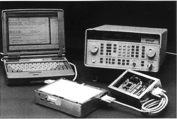
Providing a suitable package for the boards was necessary, both for ease of mobility and

convenience of operation. Figure 3-5 shows the receiver board in its package, along with

a laptop computer and a package for the voltage level conversion circuitry. The

transmitter is packaged in a similar manner as the receiver, though in a slightly larger

Figure 3-5: Receiver instrument setup. The DWN transceiver is seen on the lower right, and the voltage converter unit is on the lower left of the photograph.

While packaging the transceivers, two key issues were taken into consideration: size

and power supply. Figure 3-5 clearly shows that the packages were constructed as small

as possible to fit the transceiver, as well as a DC power source. Size is an important issue

in this project, as the measurement system must mimic any possible mobile network

siting situation. Furthermore, mobile measurement units are much easier to use in field

experiments than larger network analyzers.

An additional packaging concern was the issue of providing a power source. Since

the DWN transceivers draw approximately 45-50 mA and the radio requires a power

source of at least 3.3V, using 3 commercial AA batteries provides sufficient power.

Three AA batteries provide 4.5V as well as 500 mA-hours, therefore giving the

transceivers an approximately ten hour lifetime on a single set of batteries.

One design issue that surfaced during receiver calibration was that the microprocessor

section of the board was not regulated. This led to problems with a fluctuating RSSI

value depending on battery voltage, thereby changing the calibration curve (see Chapter

4). The reason for this was not because the DC RSSI voltage was fluctuating; rather, the

digital output values from the ATD changed depending on its voltage supply. The initial

remedy to this problem was to place a small board with a Micrel MIC5205-3.3bm5 3.3V

regulator between the battery and the transceiver. Since only the radio section contained

an on-board regulator, this solution sought to regulate both the radio power supply, as

well as the microprocessor power supply. However, the BDM12 debug module, which

obtains its power from the power supply on the board, requires more power than provided

by the regulated 3.3V supply. Therefore, instead of regulating the microprocessor power,

Chapter 4

Test Suite Characterization and Design

The previous chapter described the design and implementation of the DWN transceivers

as large-scale and small-scale propagation modeling measurement systems. While the

DWN transceivers have been used in other Draper Laboratory projects, their proper

characterization for wireless channel modeling has never been performed. It was never

necessary to identify the exact relationship between RSSI and received power, calculate

the RSSI settling time, or understand the exact antenna gains and reception patterns.

Such information, however, is critical for the purposes of using DWN as a

measurement system. This knowledge aids in understanding the process of how to

extrapolate data measured with the transceivers into useful information for the wireless

channel in question. Therefore, a thorough investigation of these issues was performed

before field tests commenced. Furthermore, based on known theory and initial field

measurements, it was necessary to formulate a test suite design in order to provide

4.1

RSSI Characterization

The centerpiece of the transceiver measurement system is the RSSI signal. While RSSI

values can be digitized on-board the receiver and then stored on a laptop computer, these

values are unitless, numerical representations of a DC voltage. The recorded data says

nothing of the exact value in decibels (dBm) or milliwatts (mW) of average power seen at

the receiver. Therefore, proper pre-measurement characterization is needed in order to

understand what the RSSI data actually means.

To perform such characterization, a calibrated Hewlett-Packard HP-E4433B signal

generator was programmed to output a similar waveform as the transmitter, i.e. a 50 kHz

FSK-modulated signal with a 58 kilobits/second symbol rate. The output of the signal

generator was then connected directly into the receiver. Signal output power was varied

from -20 dBm to -150 dBm, and then corresponding RSSI values were recorded.

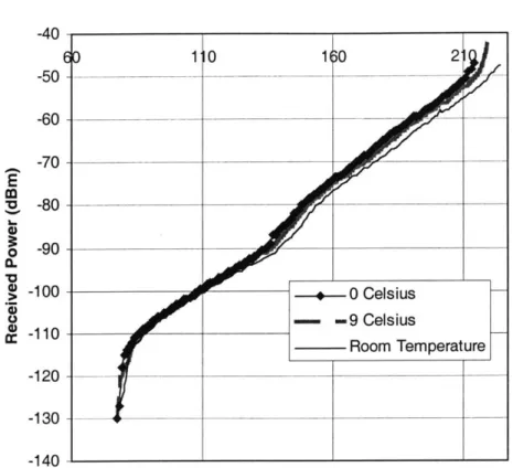
This calibration procedure was performed for three test cases: room temperature (250

Celsius), 90 and 0' Celsius. The 90 and 0' temperature measurements were taken by

placing the receiver and voltage converter both into a calibrated temperature chamber.

-40 10 160 2 -50- -60- -70-E M '. 80 -0-90 0)-100- Celsius -- -9 Celsius -0 -- Room Temperature -120 -_ -130 -_-1 -140 RSSI Values

Figure 4-1: RSSI calibration curves.

Another necessary characterization of the RSSI values is its settling time, its time

response to a change in received power. A requirement for propagation measurements is

that the settling time of the RSSI loop is less than 1/3rP of the measured correlation times.

Otherwise, observed values would be determined by the measurement hardware and not

the propagation environment. Characterization of settling time involved using the

aforementioned signal generator. In addition, an oscilloscope was set up to measure the

voltage of the receiver's RSSI signal. The output power of the signal generator was

initially set at a given value, and then stepped either up or down to a second value. The

oscilloscope was programmed in single-trigger mode to trigger once on a change in the

RSSI DC voltage. Figures 4-2 and 4-3 demonstrate a rise and fall of the RSSI signal,

. . . . . . . . . . . . . . .

.... . . . . . . . . . . . . . . . . . . . . . . .... .... . . . . . . . . . . . . . . . . . . . . . . .... . . . . . . . . . . . . . . . . . . . . . .... .... . . . . . . . . . . . . . . . . . . . . . . ....

. . . .... .... . . . ....

141,01 500MV M Soops ch i i ... 1.48, V

Figure 4-2: RSSI rise time.

.... . . . .... .... . . . .... . . . ... . . . .... . . . .... .... . . . .... I .... B .... i .... i .... i .... i .... i .... I .... i .... I .... i .... I .... I .... I .... S .... I .... I .... I .... I .... i .... i .... i .... i .... i.... . . . .... .... . . . .... . . . .... .... . . . .... . . . .... .. . . . ...

Lo= 500fliv M 300jas Chl -IL 2.69 V

In Figure 4-2, the output power of the signal generator was initially set at -120 dBm,

then stepped up to -40 dBm. In Figure 4-3, it was stepped down from -120 dBm to -40

dBm. It can be seen from the figures that the settling time of the RSSI signal is

approximately 2 ms.

4.2

Antenna Characterization

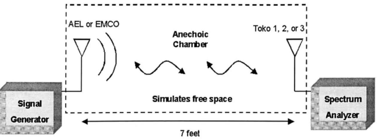
It is of utmost importance to understand what the received power values mean in the

context of field measurements. Figure 4-4 is a diagram of an arbitrary field test

configuration. In this figure, the translated RSSI signal in dBm represents the received

power at point B relative to the output power at point A. To solve for the loss in dBm

across any wireless channel, a simple equation based on Figure 4-4 can be used:

Rxpower = Txpower + GR + GT - LOSSChanne (4.1)

From Equation 4.1, to solve for channel loss, LChannei, the three unknowns are Txpower,

GT, and GR. Using a spectrum analyzer, Txpower of the transmitter was measured to be

-I dBm. Only the values of GT and GR for the DWN Toko antennas remained to be determined. Gr=3 dBm GR4 dm Wireless Channel A B Distance d TransFitter Roeceiver