HAL Id: hal-01815294
https://hal.archives-ouvertes.fr/hal-01815294
Submitted on 11 Nov 2020
HAL is a multi-disciplinary open access
archive for the deposit and dissemination of
sci-entific research documents, whether they are
pub-lished or not. The documents may come from
teaching and research institutions in France or
abroad, or from public or private research centers.
L’archive ouverte pluridisciplinaire HAL, est
destinée au dépôt et à la diffusion de documents
scientifiques de niveau recherche, publiés ou non,
émanant des établissements d’enseignement et de
recherche français ou étrangers, des laboratoires
publics ou privés.
Evolution of the cluster optical galaxy luminosity
function in the CFHTLS : breaking the degeneracy
between mass and redshift
Florian Sarron, Nicolas Martinet, Florence Durret, Christophe Adami
To cite this version:
Florian Sarron, Nicolas Martinet, Florence Durret, Christophe Adami. Evolution of the cluster optical
galaxy luminosity function in the CFHTLS : breaking the degeneracy between mass and redshift.
Astron.Astrophys., 2018, 613, pp.A67. �10.1051/0004-6361/201731981�. �hal-01815294�
Astronomy
&
Astrophysics
https://doi.org/10.1051/0004-6361/201731981 © ESO 2018
Evolution of the cluster optical galaxy luminosity function
in the CFHTLS: breaking the degeneracy between
mass and redshift
?
,
??
F. Sarron
1, N. Martinet
2, F. Durret
1, and C. Adami
31UPMC Université Paris 06, UMR 7095, Institut d’Astrophysique de Paris, 98 bis boulevard Arago, 75014 Paris, France
e-mail: [email protected]
2 Argelander-Institut für Astronomie, Universität Bonn, Auf dem Hügel 71, 53121 Bonn, Germany 3Aix Marseille Université, CNRS, CNES, LAM, 13388 Marseille, France
Received 22 September 2017 / Accepted 15 January 2018
ABSTRACT
Obtaining large samples of galaxy clusters is important for cosmology: cluster counts as a function of redshift and mass can constrain the parameters of our Universe. They are also useful in order to understand the formation and evolution of clusters. We develop an improved version of the Adami & MAzure Cluster FInder (AMACFI), now the Adami, MAzure & Sarron Cluster FInder (AMASCFI), and apply it to the 154 deg2 of the Canada-France-Hawaii Telescope Legacy Survey (CFHTLS) to obtain a large catalogue of 1371 cluster candidates with mass M200> 1014M and redshift z ≤ 0.7. We derive the selection function of the algorithm from the
Millen-nium simulation, and cluster masses from a richness–mass scaling relation built from matching our candidates with X-ray detections. We study the evolution of these clusters with mass and redshift by computing the i0
-band galaxy luminosity functions (GLFs) for the early-type (ETGs) and late-type galaxies (LTGs). This sample is 90% pure and 70% complete, and therefore our results are rep-resentative of a large fraction of the cluster population in these redshift and mass ranges. We find an increase in both the ETG and LTG faint populations with decreasing redshift (with Schechter slopes αETG= −0.65 ± 0.03 and αLTG= −0.95 ± 0.04 at z = 0.6, and
αETG= −0.79 ± 0.02 and αLTG= −1.26 ± 0.03 at z = 0.2) and also a decrease in the LTG (but not the ETG) bright end. Our large
sam-ple allows us to break the degeneracy between mass and redshift, finding that the redshift evolution is more pronounced in high-mass clusters, but that there is no significant dependence of the faint end on mass for a given redshift. These results show that the cluster red sequence is mainly formed at redshift z > 0.7, and that faint ETGs continue to enrich the red sequence through quenching of brighter LTGs at z ≤ 0.7. The efficiency of this quenching is higher in large-mass clusters, while the accretion rate of faint LTGs is lower as the more massive clusters have already emptied most of their environment at higher redshifts.
Key words. galaxies: clusters: general – galaxies: evolution – galaxies: luminosity function, mass function
1. Introduction
As the most massive gravitationally bound structures in the uni-verse, clusters of galaxies have been observed in great detail for decades. In addition to being interesting astrophysical objects, they are also a powerful probe of cosmology since galaxy cluster counts as a function of mass and redshift depend on the cosmo-logical parameters of our Universe (see e.g.Allen et al. 2011, for a review).
In this context it is important to obtain extensive samples of clusters covering wide redshift and mass ranges. It is also necessary to know the selection function of the sample with
?Based on observations obtained with MegaPrime/MegaCam, a joint
project of CFHT and CEA/IRFU, at the Canada-France-Hawaii Tele-scope (CFHT) which is operated by the National Research Council (NRC) of Canada, the Institut National des Sciences de l’Univers of the Centre National de la Recherche Scientifique (CNRS) of France, and the University of Hawaii. This work is based in part on data products produced at Terapix available at the Canadian Astronomy Data Cen-tre as part of the Canada-France-Hawaii Telescope Legacy Survey, a collaborative project of NRC and CNRS.
??The candidate cluster catalog is only available at the CDS via
anonymous ftp to cdsarc.u-strasbg.fr (130.79.128.5) or via
http://cdsarc.u-strasbg.fr/viz-bin/qcat?J/A+A/613/A67
great precision, as the cosmological constraints are obtained by comparing the observed cluster counts to the predicted ones, either from the analytical halo mass function or from N-body simulations. The development of extended imaging surveys, such as the Canada-France-Hawaii Telescope Legacy Survey (CFHTLS), provided the community with large sets of galaxy clusters observed homogeneously. It has therefore become pos-sible to detect thousands of galaxy clusters up to redshifts z ∼ 1 (e.g.Adami et al. 2010;Durret et al. 2011). The large sky cov-erage of these surveys demands an automated detection, and cluster detection algorithms are a hot topic in the literature, both for the present and next generation surveys, such as that foreseen with Euclid1, which will uncover hundreds of thousands of
clus-ters.
Many detection algorithms exist with differences in the selection function focusing either on purity or completeness. These algorithms can be separated into parametric and non-parametric. In the first category are matched filtering algorithms (e.g.Bellagamba et al. 2018), which apply a filter (e.g. Gaussian smoothing, Schechter function) to the galaxy field to highlight clusters, and red-sequence algorithms (Licitra et al. 2016), which use colour cuts to detect the linear relation between colour
1 http://www.euclid-ec.org
A67, page 1 of21
and magnitude of early-type cluster galaxies. Among the non-parametric are friend-of-friend algorithms (Farrens et al. 2011), which match close galaxies with a characteristic scale, or wavelet algorithms (Eisenhardt et al. 2008), which use the information from different scales through wavelet transformations. In the present paper we developed an improved version of the Adami & MAzure Cluster FInder (AMACFI,Mazure et al. 2007) algo-rithm which applies a smoothing to the galaxy density field in photo-z slices.
Galaxy clusters can also be used to study galaxy evolution through the distribution of galaxy magnitudes (i.e. the galaxy luminosity function, hereafter GLF) of different galaxy types. In particular the evolution of the faint end of the GLF with red-shift and mass gives insights into the effect of environment on the quenching of star formation. For nearby clusters, the faint end of red passive galaxies appears to be flat (e.g.Gaidos 1997; Paolillo et al. 2001), while it experiences a mild decrease with redshift (e.g. Smail et al. 1998; De Lucia et al. 2004;Tanaka et al. 2005;De Lucia et al. 2007;Stott et al. 2007;Gilbank et al. 2008; Rudnick et al. 2009;Vulcani et al. 2011;Martinet et al. 2015;Zenteno et al. 2016; Martinet et al. 2017). We note that some authors find no evolution with redshift (e.g.Andreon 2008; De Propris et al. 2007, 2013). RecentlyMartinet et al. (2017) ruled out the possibility that these differences could arise from surface brightness selection biases between ground- and space-based observations. Therefore, differences in the GLF faint end cannot be due to observing conditions, but are more likely to reflect variations from one cluster to another in samples of typi-cally a few tens of clusters. The dependence of the GLF on mass is less studied, mainly because of the degeneracy between mass and redshift. Indeed, at higher redshift we only detect the most massive clusters, while at low redshift we have a complete sam-ple in mass. Attempts to break this degeneracy have failed so far because of the high number of clusters required (Martinet et al. 2015,2017).
In the present study, we have improved the AMACFI cluster detection algorithm, and renamed this new version AMASCFI (Adami, MAzure & Sarron Cluster FInder). We apply it to the 154 square degrees covered by the four Wide fields of the CFHTLS survey. In particular, cluster positions and redshifts are now more accurate than the previous version used byDurret et al. (2011). We detect a total of 7100 cluster candidates up to red-shift z ∼ 1.1 and estimate the selection function of this sample by applying the same algorithm to numerical simulations based on lightcones from the Millennium simulation bySpringel et al. (2005) and modified by Henriques et al. (2012). We derive a mass for each cluster candidate using a richness–mass relation calibrated on the X-ray clusters of Gozaliasl et al. (2014) and Mirkazemi et al.(2015) that are also detected by our algorithm. We compute cluster GLFs for all galaxies, and also for early and late types separately. We study the evolution of the faint end with redshift and mass independently. And finally, we make use of the high number of clusters to break the degeneracy between mass and redshift for the first time.
The paper is structured as follows. In Sect. 2 we describe the AMASCFI code and its recent improvements. In Sect.3we study the properties of AMASCFI using simulations. In Sect.4 we compare our catalogue of cluster candidates to the literature using optically and X-ray detected clusters. In Sect.5we explain how we derived the GLFs, and the corresponding results are given in Sect.6. The results are discussed in Sect.7and the con-clusions are drawn in Sect.8. We use AB magnitudes throughout the paper, and assume a flat ΛCDM cosmology withΩM = 0.3
and h= 0.7.
2. Cluster detection
We have updated the Adami & MAzure Cluster FInder (AMACFI,Mazure et al. 2007) and applied it to the CFHTLS final data release T0007 photometric redshift (hereafter photo-z, symbol zphot) catalogues. The original AMACFI algorithm was
already applied to the CFHTLS in previous studies:Mazure et al. (2007) for the Deep1 field, Adami et al. (2010) for the T0004 data release, andDurret et al.(2011) for the Wide fields of the T0006 data release. We briefly present the main features of the method, focusing on the improvements, their motivations, and their implications.
2.1. Photometric redshift catalogue
The photo-z catalogue is obtained from the CFHTLS data release T00072.
CFHTLS T0007 photo-zs were computed in the 154 deg2sky
coverage of CFHTLS using multicolour images in the u∗g0r0i0z0
filters of MegaCam at CFHT. We note that the i0 filter had to be changed during the course of the survey. The photo-zs were obtained using the LePhare software (Arnouts et al. 1999;Ilbert et al. 2006).
Details about the method are given inCoupon et al.(2009). Briefly, the photo-zs were computed using 62 templates obtained after having optimized four templates from Coleman et al. (1980) and two starburst templates from Kinney et al. (1996), and linearly interpolated between them to better sample the colour-redshift space using the VVDS spectroscopic sample (e.g. Le Fèvre et al. 2005). A particularly crucial step of the process is the calibration of the zero-points using spectroscopic samples which help in removing biases. The resulting statistical errors on photo-zs depend on the redshifts and magnitudes of the galaxies.
Following the photo-z catalogue based on the CFHTLS T0007 data release, we define the dispersion as
σ∆zphot/(1+zs)= 1.48 × median
|∆z| (1+ zs)
!
, (1)
which is the NMAD estimator defined in Ilbert et al. (2006), with ∆zphot = zphot − zs, where zs is the
spectro-scopic redshift. The outlier rate or catastrophic failure rate η is set as the proportion of objects with |∆z| ≥ 0.15 × (1 + zs).
We make use of the value reported in the release document to choose our cuts in redshift and magnitude. For cluster detec-tion, we select galaxies in the redshift range 0.1 < zphot< 1.2 and
with magnitudes i0 < 22.5, thus keeping the dispersion below 0.05 × (1+ z) and the outlier rate below 10% in all four Wide fields.
In our analysis, we only consider galaxies that are outside the masks from TERAPIX. These masks are located around bright stars or artefacts, and mark regions of lower photometric quality. Thus photo-zs in these regions would be of poorer quality than those outside the masked regions. These masks are dealt with in the same way for cluster detection and GLF computation, i.e. by discarding objects inside the masked regions. We note that this approach is different from the oneMoutard et al.(2016) applied to the CFHTLenS, but we prefer to use the prescription from the TERAPIX team as we are using their photo-z catalogue.
2 Available at http://terapix.iap.fr/article.php?id_
2.2. AMASCFI: description of the algorithm
Our detection algorithm is based on the method described in Mazure et al. (2007). The galaxy catalogue is cut into slices of redshift, partially overlapping so as not to miss structures. Mazure et al. (2007) and subsequent studies using AMACFI chose a constant slice width of 0.1 in redshift space, each slice overlapping the adjacent ones by 0.05. In contrast, we adopt here a variable width chosen as
∆zslice= 0.05 × (1 + zslice), (2)
zslice(n+ 1) = zslice(n)+ 0.05. (3)
This enables us to better account for the noise due to photo-z sta-tistical errors, and therefore to sample a galaxy population repre-sentative of the true underlying population in each redshift slice, especially at high redshift. For example, the slice width at z= 1.1 (maximum redshift considered in our analysis) is now taken to be ∆zslice = 0.2 rather than 0.1. The galaxies were selected in
the redshift range 0.1 < z < 1.2, thus the first slice is centred at z= 0.16 and the last at z = 1.10, respectively the minimum and maximum redshifts of our detected cluster candidates. Even though the photo-z dispersion is slightly different from field to field, and depends on the redshift and magnitudes of the sources, we decided to be conservative and consider it as σ∆zphot/(1+zs) =
0.05 in all four fields, so we can treat them as homogeneously as possible.
Two-dimensional density maps are then computed in each slice using an adaptive kernel density estimator (adaptive-KDE). So far, AMACFI chose the initial size of the kernel automatically according to theSilverman(1986) prescriptions. We decided in this work to fix the initial kernel size to 1.5 Mpc.
In this way, the kernel size (diameter) of the adaptive-KDE in the densest region (corresponding to galaxy clusters) is ∼1 Mpc, which is the right smoothing scale for detecting clusters as it is the typical size of cluster cores. In fact, our previous way of choosing the smoothing scale in AMACFI was oversmooth-ing the underlyoversmooth-ing distribution and was thus more suited for supercluster than cluster detection.
The SExtractor software is then applied to the density maps to detect structures. The major modification in this step of the process is the way the detection threshold is set. This threshold is now set to a number of galaxies per Mpc2.
For this, we iteratively compute the background level (field) in galaxies per Mpc2in each slice using our density map, and set
the detection threshold to the 95% upper confidence limit on this number density followingGehrels(1986).
On the first iteration, the field is simply set to the mean galaxy number density in the entire density map. We compute the detection threshold and use SExtractor to detect overdensi-ties in the map. The background level is updated as the mean galaxy number density in the map after having removed pix-els of the density map in a disk of diameter 1 Mpc around the peak of each detected structure. This gives us a new detec-tion threshold and the process is repeated until convergence. At the end of the procedure, we obtain the final field level in the slice hnfieldi, and the detection threshold thus
quanti-fies the probability for an overdensity to be a random fluc-tuation of the background (due to chance alignment in the photo-z space).
We compute the mean number density of galaxies in a disk of 1 Mpc diameter centred at the peak of each overdensity as detected by SExtractor from our density maps and obtain a signal-to-noise ratio (S/N) of detection for each overdensity. The S/N of detection is defined as
S/N=hnclus√i − hnfieldi hnfieldi
, (4)
where hnclusi and hnfieldi correspond to the average number
den-sity of galaxies per Mpc−2in a slice of width∆z
slicefor cluster
and field area, respectively.
The overdensities thus detected in each slice are then assem-bled in larger structures (called cluster candidates in the follow-ing) using a friends-of-friends algorithm, the Minimal Spanning Tree, with a characteristic distance of 1 Mpc, as inMazure et al. (2007) (seeAdami & Mazure 1999, for the original description of the algorithm). This allows us to merge multiple detections of the same structure appearing in several adjacent redshift slices, or of large clusters presenting many substructures. The position of each candidate cluster in the (RA, Dec, zphot) space is taken to
be the mean of each of its individual merged detections weighted by its excess galaxy number density (hnclusi − hnfieldi).
3. AMASCFI selection function
In order to calibrate our method, i.e. to assess the reliability of our detections, we apply our algorithm to a set of 24 light-cones computed byHenriques et al.(2012) from the Millennium Simulation (Springel et al. 2005) and built using theGuo et al. (2011) semi-analytical model. Since then, a new set of light-cones has been built byHenriques et al.(2015) using the Planck cosmology rather than the original Millennium Simulation cos-mology (WMAP1). Even so, when comparing galaxy number counts with CFHTLS data, theHenriques et al.(2012) lightcones were in better agreement than the more recent ones. The total area of the 24 independent beams is ∼50 deg2, and thus con-tains ∼1000 haloes in the redshift range 0.1 < z < 1.2 with mass M200 > 1014M , where M200is the mass contained in a radius
r200, inside which the density is 200 times the critical density of
the Universe. Such a cosmological volume enables us to properly assess the selection function of AMASCFI. In the following, we present the modifications we applied to the lightcone to make it a fair representation of our data, and we compute the selection function of AMASCFI.
3.1. Mock catalogue modification
We converted the SDSS magnitudes of the simulated mocks to CFHTLS Megacam i0-band magnitudes following the relation
from the Megacam pages3:
iMegacam= iSDSS− 0.085 × (rSDSS− iSDSS). (5)
To make the mock galaxy catalogues from Henriques et al. (2012) comparable to our data, we need to add realistic noise to the redshift of each galaxy in the mock. Since the error on the photo-zs depends on redshift and on magnitude, we compute the mean 1σ uncertainty on individual photo-zs (as given by the LePhare software) in bins of 0.1 in redshift and 0.25 in magni-tude for the W1 field. On average, this 1σ uncertainty closely follows the statistical error computed using spectroscopic red-shifts, justifying the use of this quantity for our purpose. We decided not to add noise on the lightcone magnitudes themselves as the errors for the CFHTLS T0007 data release are below 0.01 for 95% of the sample at i0< 23, and thus negligible compared to photo-z errors.
3 http://www.cadc-ccda.hia-iha.nrc-cnrc.gc.ca/en/ megapipe/docs/filtold.html
We then apply a Gaussian error with a zero mean and a standard deviation corresponding to the mean LePhare 1σ uncertainty in the corresponding bin of the lightcones. As in Adami et al. (2010), we did not account for catastrophic errors on the photo-zs in this simplified model. The effect on clus-ter detection is expected to be small since the outlier rate stays well below 10% for the chosen magnitudes and redshift cuts.
The final step consists in applying a masking procedure representative of the one used by TERAPIX on the CFHTLS T0007. To this end, we modify the sky coordinates of the galaxies in the lightcones to match a subarea of the CFHTLS representative of the observed masks and apply the VENICE program4 to remove galaxies from the masked regions. This
step is important because masking could have an impact on the detection level of a cluster whose centre falls near a mask boundary.
We thus obtain lightcones resembling CFHTLS T0007 data in terms of masking and photometric redshift distri-bution, on which we can accurately compute our selection function.
3.2. Completeness and purity of the cluster catalogue obtained with AMASCFI
In order to assess the quality of our cluster detection we need a way to quantify how well we detect actual overdensities of galaxies and how polluted by false detections our catalogue is. Following the literature, we compute the completeness (C) and the purity (P) of our catalogue of cluster candidates to study the performances of AMASCFI. These two quantities are widely used to infer the quality of cluster catalogues. They are defined as
C= Nmatch/Ndet, (6)
P= Nmatch/Ntrue, (7)
where Ndet is the number of cluster candidates detected in the
simulation, Ntrueis the total number of haloes in the simulation,
and Nmatch the number of detected clusters matched to a halo
from the simulation.
Ideally, an algorithm should have high completeness (all clusters are detected) and high purity (all detections are actual clusters), but there is a tradeoff between the two quantities and both cannot be maximized simultaneously. The quantities are both functions of S/N cuts, which can vary depending on appli-cation. In Sect.5, for our study of GLFs, we wanted to choose a threshold that guarantees high purity so there is no contami-nation by false detections whose GLFs would resemble those of field galaxies.
We ran our detection algorithm on the simulation exactly in the same way as on the CFHTLS data, and thus obtain a cat-alogue of cluster candidates with a sky position, redshift, and detection significance. To compute the completeness and purity of the catalogue as a function of significance, redshift, and mass, we match our candidate cluster catalogue with the halo cata-logue from the simulation. The centre of each halo is taken to be its central galaxy. To match a candidate cluster with a halo, we ranked our cluster candidates by significance and the halo catalogue by halo mass and consider that they are matched when – the sky projected distance of the centres is less than the
radius r200of the halo at the halo redshift;
4 http://jeancoupon.com/venice/
– ∆z = | zhalo− zAMASCFI| ≤ 0.1 × (1+ z).
Since we are interested in detecting clusters of galaxies, we compute our completeness for haloes of mass M200> 1014M .
However, computing purity with the same mass threshold would be too drastic. Indeed, some of our detections may correspond to haloes of smaller masses (galaxy groups) and thus not be false detections per se. This arises from the intrinsic scatter (σint) that exists between halo mass and cluster richness. This
scatter is found to be of the order 0.3 dex in the local Universe (Andreon & Bergé 2012). This means a halo with mass ∼3σint
below the 1014M
threshold could have the same richness as
a halo of 1014M . Following these considerations, we compute
the purity of our candidate cluster catalogue for haloes of mass M200> 1013M .
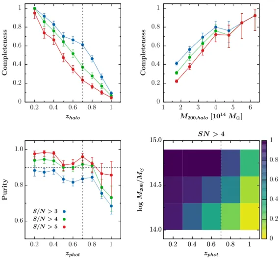
In Fig. 1, we show the cluster completeness as a func-tion of redshift for haloes of mass M200 > 1014M and as a
function of halo mass in the entire redshift range 0.15 < z ≤ 1.1, for different S/N cuts. Error bars represent the 1σ confi-dence limit of a binomial distribution followingGehrels(1986). The bottom left panel in Fig. 1 shows the purity of our cat-alogue, while the bottom right panel breaks the degeneracy between mass and redshift, showing the completeness as a func-tion of both parameters for S /N > 4. The error on the redshift assigned to a candidate cluster by AMASCFI (zAMASCFI) is
esti-mated using the NMAD estimator. We find σzclus = 0.018 ×
(1+ z) for haloes of mass M200 > 1013M . When considering
only matched haloes of mass M200> 1014M , this reduces to
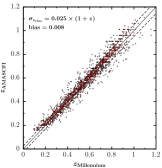
σzclus = 0.018 × (1 + z). This is illustrated in Fig. 2 where we
plot zAMASCFI vs. the true redshift of the matched halo in the
simulation zMillennium.
When computing completeness and purity as a function of redshift only, bins include clusters with a redshift ±2 × σzclus
from the central redshift of the bin, where σzclus = 0.025 × (1 + z)
is the statistical error on cluster redshift. The first bin is centred at z= 0.2 and the last at z = 1.0, with an offset of 0.1 between bins. When computing completeness as a function of mass, bins include clusters with a mass ±7.5 × 10¹³M from the central
mass of the bin. The first bin is centred on 1.75 × 10¹⁴M and
consecutive bins are offset by ±7.5 × 10¹³M , so that bins
par-tially overlap and smooth the selection function. The last bin in mass only includes a lower limit and so includes all clusters more massive than 5 × 10¹⁴M
.
When breaking the degeneracy between redshift and mass, we consider three bins in each parameter. This is done so that each bin is sufficiently populated to have reliable statistics. We choose to use the three redshift bins [0.1, 0.3[, [0.3, 0.5[, and [0.5, 0.7[ and mass bins ]1014M
, 1014.3M ], ]1014.3M ,
1014.6M ], and ]1014.6M , ∞ [. The mass bins were built to
have the same size in logarithmic space and so that the highest mass–highest redshift bin contains a sufficiently large number of clusters.
For the three S/N cuts considered, the purity is >70% in the entire redshift range, and >80% for zclus ≤ 0.8. The
com-pleteness is >70% for the most massive clusters (log M200/M >
14.6) in the entire redshift range, while being always ∼70% for all clusters (log M200/M > 14) up to zclus = 0.4. As the
redshift increases, large differences can be seen in the com-pleteness depending on the S/N cut considered. The complete-ness becomes low (<30%) for all S/N cuts for zclus > 0.8.
This is due to the increasing errors on the photo-zs with redshift.
Since we want to use our cluster catalogue to compute cluster GLFs, the primary criterion is a high purity of the catalogue. We
0 0.2 0.4 0.6 0.8 1 0.2 0.4 0.6 0.8 1 0 0.2 0.4 0.6 0.8 1 1 2 3 4 5 6 0.6 0.8 1.0 0.2 0.4 0.6 0.8 1 14.0 14.5 15.0 0.2 0.4 0.6 0.8 1 Completeness zhalo Completeness M200,halo[1014M ] Purit y zphot S/N > 3 S/N > 4 S/N > 5 log M 200 / M zphot SN > 4 14.0 14.5 15.0 0.2 0.4 0.6 0.8 1 0 0.2 0.4 0.6 0.8 1
Fig. 1. Selection function of AMASCFI using the Millennium modified lightcones of Henriques et al.(2012). Top left: completeness as a function of redshift for haloes of M200 > 1014M . Top right: completeness as a function of halo mass. Bottom left: purity as computed for
haloes of mass M200 > 1013M . In these three panels, blue, green, and red points respectively show the results for S /N > 3, S /N > 4,
and S /N > 5. Bottom right: two-dimensional histogram of the completeness in the (redshift, mass) parameter space for cluster candidates with S /N > 4. The vertical dotted line at z = 0.7 shows the cut applied to compute GLFs (see Sect. 3.3) and the horizontal line the 90% purity limit.
thus choose a cut at S /N > 4 that guarantees a purity >90% up to zclus= 0.8. For this very pure cut, we compute the completeness
as a function of both redshift and halo mass (bottom right panel in Fig.1). For the most massive bin (log M200/M > 14.6), the
completeness is >70% up to zbin = 0.8 and then drops. A 70%
completeness threshold is reached up to zbin = 0.6 for the
inter-mediate mass bin (14.3 < log M200/M ≤ 14.6) and zbin = 0.4
for the lowest mass bin (14 < log M200/M ≤ 14.3). In
addi-tion to its high purity, the cluster candidate catalogue used for the GLF computation is therefore also representative of clusters with mass M200> 1014M .
3.3. Mass, redshift, and S/N cuts for GLFs
In the following sections of the paper, we study the proper-ties of cluster GLFs, using the cluster candidates detected with AMASCFI. A study of this kind is usually done with a catalogue of confirmed clusters because the results are relatively sensitive to contamination by false detections. Thus, to study the cluster candidate GLFs, we need to choose cuts in S/N, redshift, and richness (or equivalently mass), which ensures a high purity. At the same time, we would like to keep the completeness to high enough levels so that the population of cluster candidates under consideration can be considered as fairly representative of the true cluster population.
Using the selection function we computed on simulations, we chose to cut our final catalogue for GLF computation at S /N > 4, z < 0.7 and M200> 1014M . This ensures a purity higher than
90% in the full redshift range (see bottom left panel in Fig.1) and a completeness greater than 50% in all the redshift and mass bins considered. The lower mass limit enables us to probe low-mass galaxy clusters, and the redshift range to study the cosmic evolution of the cluster properties.
4. AMASCFI applied to the CFHTLS T0007 data release
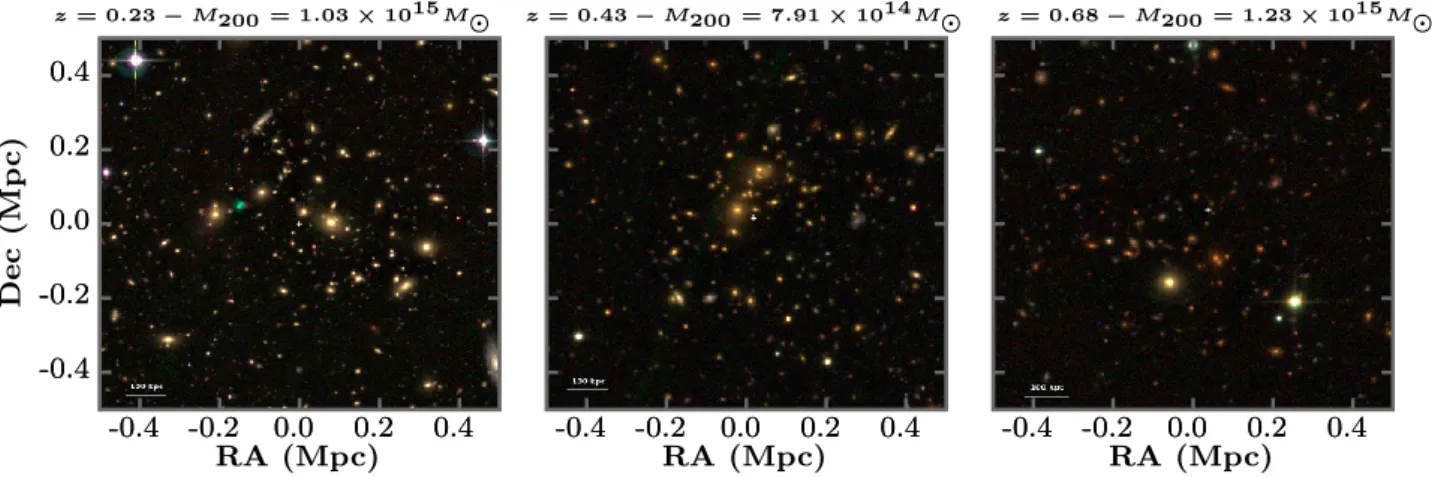
When applying AMASCFI to the four Wide fields of the CFHTLS T0007 data release photo-z catalogue, we detect 7100 cluster candidates at S /N > 3 in the redshift range 0.15 < z < 1.1. The full catalogue will be made available at the CDS. Optical images of three rich clusters are shown in Fig. 3 for illustration. In the following sections, we will compare our candi-date cluster catalogue to previously published cluster catalogues on the Wide fields of CFHTLS. We will first make a compar-ison with other optically detected cluster candidate catalogues fromLicitra et al.(2016) andFord et al.(2015), and with X-ray detected cluster catalogues from Gozaliasl et al. (2014) and Mirkazemi et al.(2015).
0 0.2 0.4 0.6 0.8 1 1.2 0 0.2 0.4 0.6 0.8 1 1.2 σzclus= 0.025× (1 + z) bias = 0.008 zAMASCFI zMillennium
Fig. 2.zAMACSFI vs. zMillennium for all cluster candidates with S /N > 3
matched in theHenriques et al.(2012) lightcones. Black points are for all clusters and groups with mass M200 > 1013M , while red points
are only for clusters with mass M200 > 1014M . The black line is the
identity line. The dashed lines are ±σzclus= 0.025 × (1 + z).
4.1. Matching AMASCFI cluster candidates with other optically selected cluster candidates
There are two public catalogues of optically selected cluster candidates, obtained from the CFHTLS observations, although both use the CFHTLenS photometric catalogue extracted from the data rather than the TERAPIX catalogue. The first is the Ford et al.(2015) cluster catalogue. It covers the four Wide fields of the CFHTLS and was obtained using the 3D-MF algorithm developed byMilkeraitis et al.(2010). The 3D-MF algorithm is a matched filter algorithm that assumes a cluster radial profile and luminosity function and detects clusters in overlapping slices of redshift. The full published catalogue contains 22 694 cluster candidates with significance σFord > 3.5 in the redshift
range 0.2 < z < 1.0.
To match the two catalogues we use the same matching procedure as in Sect. 3.2, except for the maximum radial projection between the centres of two matched clusters, which is fixed to 2 Mpc to account for the large errors on the sky position of cluster candidates and because we have no estimate of r200 in the observations. When matching our catalogue with
the full 3D-MF catalogue, we find 5285 cluster candidates in common, meaning that 75% of AMASCFI clusters have a counterpart in the 3D-MF catalogue. This agrees well with the purity of AMASCFI at S /N > 3, that we computed using the Millennium simulation (see Sect.3.2), considering the 3D-MF cluster catalogue has high completeness (Milkeraitis et al. 2010). If we trim the 3D-MF catalogue to σFord > 5 (which
corresponds to ∼1.5 × 10¹³M ) and σFord > 10 (which
corre-sponds to ∼1014M
; Ford et al. 2015), there are respectively
6544 and 282 clusters left in the redshift range 0.2 < z < 1.0. AMASCFI respectively detects 3521 (∼54%) and 260 (∼92%) of these.
Licitra et al.(2016) developed the RedGOLD cluster detec-tion algorithm, based on the search for red-sequence galaxy overdensities. The search is done in slices of redshift, where the red-sequence colour is predicted using stellar population
models. To select their cluster candidates, they impose a Navarro–Frenk–White (NFW) profile, and compute a richness estimator λRedGOLD for each candidate. RedGOLD was applied
to the CFHTLS W1 field. Their published catalogue includes 652 cluster candidates in the redshift range 0.14 ≤ z < 1.2. Out of the 7100 cluster candidates detected by AMASCFI, 2951 lie in the CFHTLS W1 field.
We use the same matching procedure as for the Ford et al. (2015) catalogue. Out of the 652 RedGOLD cluster candidates, 510 are also found by AMASCFI (78%), a result in good agreement with the ∼80% purity of both catalogues at the significance cuts used. If we only consider AMASCFI cluster candidates with S /N > 5.5, to have a comparable number of candidates in both catalogues (663 for AMASCFI and 652 for RedGold), 45% of cluster candidates are matched. Since the RedGOLD catalogue has an announced completeness of ∼70% and AMASCFI has less than 50% (at this S/N cut) in the redshift range considered, this is expected.
4.2. Matching AMASCFI cluster candidates with X-ray detected clusters
We also compare our candidate cluster catalogue with two X-ray detected cluster catalogues provided by Gozaliasl et al.(2014) andMirkazemi et al.(2015), both obtained from XXM-Newton observations. TheGozaliasl et al.(2014) catalogue covers an area of 3 deg2inside the CFHTLS W1 field and includes 135 X-ray
detected groups and clusters up to z= 1.1, while theMirkazemi et al.(2015) catalogue was built by pointing at given optically selected cluster candidates; it includes 196 X-ray detected groups and clusters up to z= 1.1 in the CFHTLS W1, W2, and W4.
Both catalogues provide M200 for each cluster, obtained by
applying the scaling relation between weak lensing mass and X-ray luminosity (M200,W L− LX) obtained by Leauthaud et al.
(2010). We recalibrate these masses according to the Kettula et al. (2015) scaling relation as it presents the advantage of measuring the weak lensing mass for individual clusters, while Leauthaud et al.(2010) stacked the lowest mass clusters in quite poorly populated bins.
The intrinsic scatter in the relation and the errors on the fit parameters are propagated to obtain the errors on the mass estimates. Finally, we translated cluster masses into our own cosmology (only H0= 70 km s−1Mpc−1differs).
When comparing the mass distributions obtained from the M200,W L− LX relations to that obtained by applying AMASCFI
to the Millennium simulation, we find that theLeauthaud et al. (2010) M200,W L− LX relation underpredicts the number of
clus-ters with M200> 1014M , while the number of clusters predicted
by the Kettula et al. (2015) relation is in good agreement. Parroni et al. (2017) recently found similar results, with the Leauthaud et al.(2010) normalization being too low, when com-pared to their CFHTLenS data, especially in the range M200>
1014M
, which is of main interest in our study. These arguments
lead us to believe that our choice to use Kettula et al.(2015) M200,W L− LX scaling relation in our analysis was the correct
one.
Having obtained these mass estimates, we can match our cluster candidates with the X-ray detected clusters and look how well AMACSFI redetects them as a function of mass and red-shift. However, neither Gozaliasl et al. (2014) nor Mirkazemi et al.(2015) provide the completeness of their catalogue for given mass and redshift. Thus they cannot be used to properly compute a selection function of our algorithm, but only give us insights into how AMASCFI performed on the CFHTLS T0007 data. We
-0.4 -0.2 0.0 0.2 0.4 -0.4 -0.2 0.0 0.2 0.4 -0.4 -0.2 0.0 0.2 0.4 -0.4 -0.2 0.0 0.2 0.4 Dec (Mp c) RA (Mpc) z = 0.23− M200 = 1.03 × 10¹⁵M -0.4 -0.2 0.0 0.2 0.4 -0.4 -0.2 0.0 0.2 0.4 RA (Mpc) z = 0.43− M200 = 7.91 × 10¹⁴M -0.4 -0.2 0.0 0.2 0.4 RA (Mpc) z = 0.68− M200 = 1.23 × 10¹⁵M -0.4 -0.2 0.0 0.2 0.4
Fig. 3.griimages of three rich cluster candidates in the CFTHLS W1 field, centred on the AMASCFI cluster centres.
13.5 14 14.5 15 0.2 0.4 0.6 0.8 log M 200 / M zclus 13.5 14 14.5 15 0.2 0.4 0.6 0.8
Fig. 4.Matching of our cluster candidates obtained with AMASCI and X-ray groups detected in the same area of the W1 field byGozaliasl et al.
(2014). Blue filled squares are clusters and groups from theGozaliasl et al.(2014) catalogue. Black empty squares are clusters also detected by AMASCFI. See text for details.
use the same matching procedure as in Sect.3.2, using for r200
the value given in the original catalogue.
There are 68 groups in theGozaliasl et al.(2014) catalogue with z < 0.75. In the same area AMASCFI detects 51 clusters at S/N > 4 and z < 0.7, 23 of them also being in theGozaliasl et al. (2014) catalogue (see Fig. 4). In addition, AMASCFI detects all but two X-ray clusters with M200 > 1014M up to
z = 0.6. The Mirkazemi et al. (2015) catalogue contains 130 clusters with z < 0.75, while AMASCFI detects 1872 clusters at S /N > 4 and z < 0.7 in the W1, W2, and W4 fields. There are 66 clusters in common between the two catalogues (see Fig.5). When using the detections in common with the X-ray catalogues, the statistical error on the redshifts of the AMASCFI clusters is the same as that computed on the Millennium simulation (σclus= 0.025).
We did not match our cluster candidates with X-ray detected clusters from XXL because the published catalogue fromPacaud et al. (2016) only includes massive clusters and thus covers a mass range less interesting than theGozaliasl et al.(2014) and Mirkazemi et al.(2015) catalogues combined.
13.5 14 14.5 15 0.2 0.4 0.6 0.8 log M 200 / M zclus 13.5 14 14.5 15 0.2 0.4 0.6 0.8
Fig. 5. Matching of our cluster candidates obtained with AMASCFI and X-ray groups/clusters detected in the W1, W2, and W4 fields by
Mirkazemi et al.(2015). The symbols are the same as in Fig.4.
4.3. Mass-richness calibration
The richness of a cluster is known to be a proxy for its mass, which is not measurable directly. Having an estimator with as small a scatter as possible in the mass-richness relation is of great interest to study the dependence of cluster properties on mass. We can use our GLF computation method (see Sect.5) to derive such a richness estimator for our cluster candidates.Rykoff et al. (2012) showed that including blue cluster members in their rich-ness estimate increased scatter in the LX-richness relation from
σlnLX|λ= 0.63 to σlnLX|λ= 0.72 at the 2σ level. With this result
in mind, we decided to build our richness estimator based on the cluster GLF of early-type galaxies (ETGs). Our goal was to count the number of red ETGs brighter than a given absolute magni-tude, so we can directly use the counts in absolute magnitude that are also used to build our GLF.
We computed the ETG GLF in a 1 Mpc radius. We then summed the number counts in absolute magnitude bins, after removing field counts, for galaxies brighter than 0.2 × L∗, i.e. M < M∗+ 1.75. Here M∗ (respectively L∗) is the
characteris-tic absolute magnitude (luminosity) of a cluster, and is obtained from a Schechter fit to the GLFs stacked in redshift bins. We
0 20 40 60 80 100 0 20 40 60 80 100 RAMASCFI λRedGOLD
Fig. 6. Comparison of the AMACFI (RAMAS CFI) and RedGOLD
(λRedGOLD) richness estimates.
took a constant M∗equal to the mean M∗over our redshift range:
hM∗i
z= −22.6.
The 90% completeness limit of our sample being i0= 23,
we were able to reach M∗+ 1.75 up to z = 0.7. Thus, our rich-ness estimator was homogeneous up to z= 0.7, and we did not compute the richness for clusters with higher redshifts.
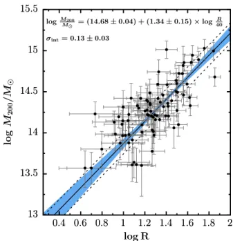
We calibrated our richness R to X-ray derived cluster masses, using the catalogues fromGozaliasl et al.(2014) andMirkazemi et al. (2015) to infer the mass for all our cluster candidates up to z= 0.7. We used the catalogue of matched clusters derived in Sect.4.2and fitted the M200− R relation as
log10 M200 M = β + α × log10 R 40, (8)
where the pivot value for richness is taken to be 40 as in, e.g. Licitra et al.(2016);Rykoff et al.(2012).
Figure7 shows the mass-richness relation for the 82 clus-ters detected by AMASCFI with an X-ray counterpart in either theGozaliasl et al.(2014) orMirkazemi et al.(2015) catalogues up to zAMASCFI = 0.7. The fit was done using the John Meyers
python implementation of the linmix_err IDL routine (Kelly 2007) with a default superposition of three Gaussians. This Bayesian approach considers that the errors follow a Gaussian distribution, while the error on the richness is Poissonian by nature. However, we verified that every cluster has a high enough richness (R > 10) for the Poisson law to be closely approximated by a Gaussian. We note that four clusters only reach R > 5; we kept them in the analysis as they should not significantly affect the errors on the fit and improve the representation of low-mass clusters. We obtain β= 14.68 ± 0.04, α = 1.34 ± 0.15, and the intrinsic dispersion σint= 0.13 ± 0.03 dex.
Comparing our scaling relation with the literature is not straightforward since different richness estimators will yield different scaling relations. However, our definition of rich-ness is similar to that computed by the RedGOLD algorithm (Licitra et al. 2016), i.e. counting bright ETGs in a given radius. The main difference is that contrary to Licitra et al. (2016), who scale the radius in which the richness is computed iter-atively, we fixed this radius to 1 Mpc. We compare the two estimators in Fig.6, plotting the AMASCFI richness estimator RAMASCFIvs. the RedGOLD richness estimator λRedGOLDfor the
13 13.5 14 14.5 15 15.5 0.4 0.6 0.8 1 1.2 1.4 1.6 1.8 2 log M 200 / M log R 13 13.5 14 14.5 15 15.5 0.4 0.6 0.8 1 1.2 1.4 1.6 1.8 2 logM200 M = (14.68± 0.04) + (1.34 ± 0.15) × log R 40 σint= 0.13± 0.03
Fig. 7. Mass-richness relation for clusters in common between AMASCFI (at S /N > 4 and z < 0.7) and either theGozaliasl et al.
(2014) orMirkazemi et al. (2015) catalogues. The mass M200 of the
X-ray detected clusters was obtained applying theKettula et al.(2015) M200− LXscaling relation. The fitted relation is shown at the top of the
figure. The solid black line is the median relation, while the blue zone shows the 68% confidence on the fit parameters. The dashed lines show the intrinsic scatter in the relation.
matched clusters. We find a good correlation between them, the AMASCFI richness being 16% lower in the mean than RedGOLD richness.
Parroni et al.(2017) used the RedGOLD catalogue to com-pute a mass-richness scaling relation from weak-lensing masses and their results are similar to ours, but with lower α and β. This is expected because our richness estimates are lower than theirs. We also find a similar intrinsic scatter σint, showing that both
estimators are similarly good mass proxies, as previously argued byAndreon & Hurn(2010).
Using the fit result, we can infer the posterior probability dis-tribution for the mass of each candidate cluster for which we have computed a richness. As discussed previously (Sect.4.2) this gives us a mass distribution for our cluster catalogue that is in good agreement with that derived from applying AMASCFI to simulations.
5. Cluster galaxy luminosity functions
We wanted to study the evolution of the cluster luminosity func-tions (GLFs) with redshift and their dependence on cluster mass. Our method for computing GLFs is based on the method devel-oped in Martinet et al. (2015) (hereafter M15) and adapted to the specificity of CFHTLS T0007 data. Taking advantage of the size of our sample, we were able to break the degeneracy between mass and redshift. We computed GLFs of our cluster candidates in the i0 rest frame band using photo-z informa-tion to estimate the cluster membership of galaxies. We used the i0 band because for photo-z computation, the full T0007
catalogue was cut at i0 < 24, so it is complete in this band only. Martinet et al. (2015) showed that GLFs behave simi-larly in the V, R, and I band, so our conclusions are quite general.
5.1. Completeness limit
One key point when computing GLFs is to properly define the 90% completeness limit of the sample. The CFHTLS data have the advantage of being homogeneous across the whole field and the 80% completeness limits were computed by TERAPIX. However, these depth limits show substantial variations from tile to tile. Indeed, the deepest tile has an 80% completeness limit of ci0,80%= 24.07, while the shallowest has c0
i,80% = 23.30 (the
mean being ci0,80% = 23.72). To obtain the 90% completeness
limit, we used data provided in T0007 of the CFHTLS, where the completeness limit is assessed using simulations.
We decided to be conservative and to take the same 90% completeness limit in all the fields: ci0,90%= 23.0. This has two
main advantages: the first is that we were able to study homo-geneously our entire sample, and the second is that photo-zs become noisier for magnitudes fainter than i0= 23 (σ∆zphot/(1 +
zs) ∼ 0.07 and η >∼ 10–15%), so that considering fainter
galaxies may have affected the quality of our analysis.
This apparent magnitude completeness limit is translated to an absolute magnitude completeness limit by adding the distance modulus and k-correction. We used the k-corrections computed by LePhare. The software computes the theoretical k-correction from the best fit template and best estimated redshift of the galaxy. Here we want our completeness value to be correct for all types of galaxies. We thus selected all the galaxies in 0.05 × (1+ zclus) and computed for each template the mean
k-correction. For our result to hold for both early- and late-type galaxies (ETGs and LTGs, see Sect. 5.4), we computed the mean k-correction over ETG templates and LTG templates and the final value was taken as the maximum of these two quantities.
5.2. Galaxy luminosity function computation
To compute our GLFs, we used the final catalogue containing all the relevant information for each galaxy: position in the sky, photo-z, and apparent and absolute magnitudes in i0band. For each cluster, we selected galaxies in a cylinder of radius 1 Mpc and length ±2 × 0.05 × (1+ zclus). Part of these galaxies are not
cluster members but rather background or foreground galaxies, so we needed to remove the field contribution because the photo-zstatistical error of ∼0.05 × (1+ zs) is larger than the typical size
of a cluster ∼0.001 × (1+ z) (see e.g.Evrard et al. 2008). We call the galaxies thus selected the candidate cluster galax-ies in the following. Once this selection was done, we fixed all the candidate cluster galaxies to the cluster redshift and re-ran LePhare without fitting the photo-zs (parameter ZFIX). LePhare only fits the best template, which might be different when we force zgal= zclusas discussed inM15. This allows us to determine
the template, k-correction, and hence the absolute magnitude of each candidate cluster galaxy more accurately, as these are redshift dependent properties.
We then subtracted the field contribution from our candidate cluster galaxies. The field galaxies are defined for each redshift slice as galaxies more than 2 Mpc away from any detected cluster in the slice. We normalised the field to each cluster area before subtracting galaxy counts.
One point that needs to be dealt with carefully is that field galaxies have k-corrections computed at their own redshift, while for the candidate cluster galaxies the k-correction was computed at the cluster redshift. An error in the k-correction could move a galaxy from one absolute magnitude bin to another in our GLF, thus distorting the actual GLF. To avoid this effect, we
removed the field contribution in bins of apparent magnitude. We counted candidate cluster galaxies and field galaxies in bins of 0.5 magnitude and applied a weight to all galaxies in the bin equal to the ratio of cluster to field galaxies in the bin. Once field counts were subtracted, we normalised our GLFs to 1 Mpc2. This
was done so that we can compare the GLFs at different redshifts. 5.3. Stacking the GLFs
Because of low number counts, individual cluster GLFs are noisy. Thus, we cannot use them to infer the dependence of the faint-end slope of the GLF with mass and redshift. To increase our S/N, we stacked our GLFs in bins of redshift and mass. Stacking was done as inM15using the standard Colless method (Colless 1989). The idea is to average cluster galaxy counts in each absolute magnitude bin, including all clusters that are 90% complete in this bin. Clusters first have to be normalized to the same area and to a fixed richness. We normalised all clusters to 1 Mpc2. For the richness we used our estimator described in
Sect.4.3.
The main advantage of this method compared to a classical average of GLFs is that we are able to use as much information as possible. Indeed, with a classical method, the average would only be done in the absolute magnitude bins which are 90% complete for all the clusters considered, thus limiting our capacity to probe the faint-end in a given redshift range.
Galaxy counts and their errors are summed following Eqs. (9) and (10), respectively, where N( j) and σ( j) are the stacked galaxy counts and galaxy count errors in magnitude bins j, the index i indicates single cluster values, Si is the area of
cluster i, Nc( j) is the number of clusters in the bin j, and N0,i
and hN0( j)i are the richness of cluster i and the mean richness of
clusters in the j bin: N( j)=hN0( j)i Nc( j) X i Ni( j) SiN0,i , (9) σ( j) = hN0( j)i Nc( j) v t X i σi( j) SiN0,i !2 . (10)
To retain the Poissonian distribution of the counts, we weight the individual variances by the square of the cluster area, as for the galaxy counts, and not simply the area. We did not take into account the clustering error in our estimation of the individ-ual variances, because it is negligible compared to the Poisson error. We fit the stacked i0band GLFs with a Schechter function
(Schechter 1976)
N(M)= 0.4 ln(10) φ∗h100.4(M∗−M)iα+1e−100.4(M∗ −M), (11) where φ∗ is the characteristic number of galaxies per unit
volume, M∗ the characteristic absolute magnitude, and α the faint-end slope of the GLF. The fit is done with a χ2
minimiza-tion. The error bars on the parameters correspond to the 1σ confidence level and are computed from the covariance matrix, evaluated at the best parameter values. These single parameter error bars include the effects of correlations with other parame-ters. As inMartinet et al.(2017), we convert the final χ2value in
a confidence probability p assuming a χ2distribution with three degrees of freedom (α, M∗, φ∗): p(χ2, 3) = √2 π √ π 2 erf r χ2 2 − exp −χ 2 2 !r χ2 2 . (12)
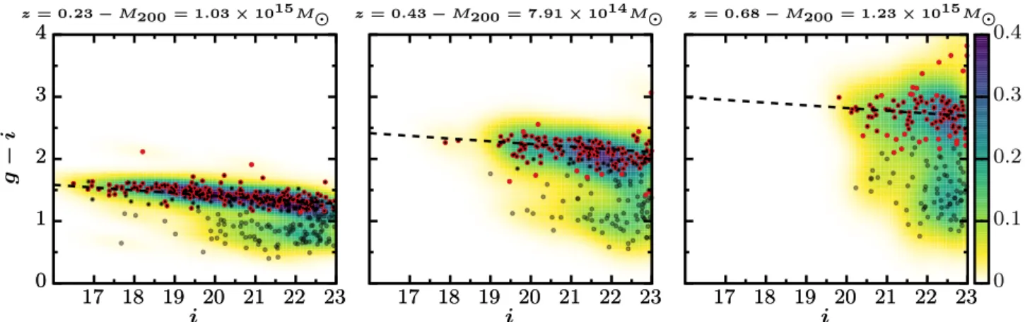
0 1 2 3 4 17 18 19 20 21 22 23 17 18 19 20 21 22 23 17 18 19 20 21 22 23 g − i i z = 0.23− M200 = 1.03 × 10¹⁵M 0 1 2 3 4 17 18 19 20 21 22 23 i z = 0.43− M200 = 7.91 × 10¹⁴M 17 18 19 20 21 22 23 i z = 0.68− M200 = 1.23 × 10¹⁵M 17 18 19 20 21 22 23 0 0.1 0.2 0.3 0.4
Fig. 8.Colour-magnitude diagram (g-i) vs. i for three rich clusters in the CFHTLS W1 field. Empty black circles are candidate cluster galaxies. The underlying distribution is their normalized density. In red are galaxies selected as ETGs at the cluster redshift by LePhare. Smaller black points are galaxies selected as RS members, i.e. lying ±0.3 from the best fit RS.
new template n um b er
old template number 0 10 20 30 40 50 60 0 10 20 30 40 50 60
Fig. 9. Comparison of best fit templates for each candidate cluster galaxy for a rich candidate cluster at zclus= 0.35. The blue and red points
respectively show the new templates considered as late-type galaxies (LTGs) and early-type galaxies (ETGs). The black squares show galax-ies moving from ETG to LTG and vice versa. The old template is the best fit template in the original catalogue (the redshift is free to vary during the SED fitting), while the new template is the best fit template when we force the galaxy to be at the cluster redshift (zphot,gal = zclus).
This illustrates that template fitting of galaxies is quite sensitive to small changes in redshift, but that classifications are relatively stable.
We wanted to study the dependence of the GLFs with red-shift and cluster mass. So we binned our cluster candidates in this 2D parameter space, and stack the clusters in each bin using the Colless method described above. As mentioned in Sect.3.2, we chose to use the three redshift bins [0.1,0.3[, [0.3,0.5[, and [0.5,0.7[. These redshift bins are wide enough to be well pop-ulated and narrow enough to study the redshift dependence of the GLFs. We also use the three mass bins ]1014M , 1014.3M ],
]1014.3M
, 1014.6M ], and ]1014.6M , ∞ [.
5.4. Early- and late-type galaxies
To better understand the properties of clusters, it is interesting to study their different galaxy populations. Ideally this prob-lem could be dealt with in a complex manner by classifying
many types of galaxies (early quiescent ellipticals, late dust-free spirals, late dusty spirals, starburst galaxies, early spirals, galax-ies transiting from late spiral to early elliptical, etc.). However, the automatic classification of galaxies in such a complicated scheme is very difficult. Indeed, the more templates/categories we try to fit the data with, the more degenerate the classification. We used LePhare templates to classify galaxies as ETGs and LTGs. We recall that the LePhare SED fitting for cluster members is done using the ZFIX parameter with zgal fixed at
zclus. We verified that this small redshift shift does not
signif-icantly affect our ETG–LTG separation by comparing cluster best fit galaxy templates before and after fixing galaxy red-shifts. This is shown in Fig. 9 for a rich cluster at z = 0.35. We find that the best fit template is quite sensitive to a moder-ate change in redshift, with most galaxies having their templmoder-ates changed, yet the classification as ETG or LTG only changes for ∼5% of the galaxies. This is due to the degeneracy between the spectra of ETGs and of LTGs with a dust component. It is a well-known limitation of template fitting codes, but since the proportion of these objects stays low it should not affect our conclusions.
Our classification somehow differs from the usual red-sequence (RS) classification used in most of the literature. Understanding how the two compare is important to properly compare our results with previous studies. First, we would like to point out that previous studies also used techniques that differed from each other. Some used a simple colour cut (Popesso et al. 2006). Other studies fitted a proper red sequence with a tilt in a colour-magnitude diagram, but either with a fixed slope (e.g. Martinet et al. 2015;De Lucia et al. 2007) or varying both the slope and the intercept (e.g.Cerulo et al. 2016;De Propris et al. 2015). To compare both classifications, we fitted a RS to each of our clusters in (g − i) vs. i using
g − i = −0.0436 × (i − m∗
i)+ b, (13)
where the slope is fixed at −0.0436, as inMartinet et al.(2015), and the intercept is computed at m∗
i, which is the observed
characteristic magnitude computed from the mean M∗ over our redshift range: hM∗iz = −22.6. As a first guess for the
inter-cept, we interpolated the elliptical galaxy colour fromFukugita et al.(1995) to each cluster redshift and selected a wide prelimi-nary RS with a width of 0.6 in magnitude. For the galaxies thus selected, we then fitted a RS with a free ordinate b and selected galaxies at ±0.3 in magnitude around this final RS. An example
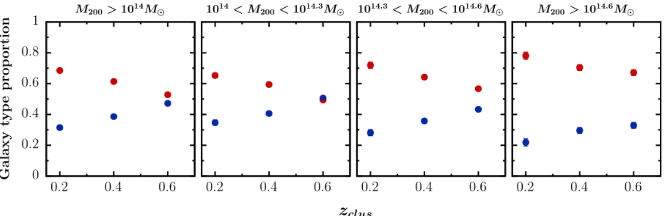
0 0.2 0.4 0.6 0.8 1 0.2 0.4 0.6 0.2 0.4 0.6 0.2 0.4 0.6 0.2 0.4 0.6 Galaxy typ e prop ortion M200> 1014M 1014< M200< 1014.3M
z
clus 1014.3< M 200< 1014.6M M200> 1014.6MFig. 10.Mean proportion of ETGs (red) and LTGs (blue) brighter than M∗+ 1.75 in cluster candidates as a function of redshift. The left panel
shows the redshift evolution for all cluster candidates with mass M200> 1014M . The other three panels segregate the cluster candidates in mass
bins as defined in the text. Error bars represent the standard error on the mean.
of the RS fit and galaxy selection is shown in Fig.8for three rich clusters at different redshifts. We checked the robustness of the fit on these clusters by changing by 0.2 the colour used for pre-selection based onFukugita et al.(1995) and allowing the slope to vary.
Both checks prove our selection to be robust, as the slope only changes by 0.01 and the intercept by 0.05. Thus, only a few galaxies change their population type compared to our final RS selection. This RS selection is compared to our ETG/LTG classification in Fig. 8. One can see that at low redshift our selection discards part of the RS selected galaxies, especially at faint magnitudes, while the two methods agree well at high redshift. The difference at low redshift arises because some of the galaxies in the RS are actually LTGs reddened by dust. With the observing bands we have, it is hard for LePhare to properly segregate between ETGs and dusty-LTGs for a given galaxy. However, statistically speaking, our selection is closer to a true quiescent vs. star-forming selection than the RS, because it is less polluted by these dusty-LTGs. Quantitatively, for all three clusters 99%, 92%, and 73% of our ETGs are also RS galaxies. Inversely, there are, from low to high red-shift 65%, 80%, and 96% of RS galaxies that are classified as ETGs.
The final effect on the GLF is hard to predict since the field of a RS selection has higher number counts than the field of an ETG selection. To properly investigate how the two methods compare with regard to the stacked GLFs, we thus built the RS GLFs for all clusters and compared the RS stacked GLFs to the ETG stacked GLFs in our nine bins of masses and redshifts. This is illustrated in Fig.A.1. We see that at high redshift the two selec-tions are in good agreement for all mass bins, so our conclusions concerning the evolution of the ETG GLF are not affected by the chosen selection criterion.
6. Results
In this section we present the results of the GLFs of our clus-ter sample. We first analysed how the fraction of ETGs depends on redshift and mass. We then studied the stacked GLFs of our cluster sample. As pointed out in Sect. 3.3, we stacked clus-ter candidates with a mass larger than 1014M and redshift
0.15 < zclus < 0.7 in corresponding redshift and mass bins. We
study in particular how the parameters of our fitted Schechter functions depend on redshift and mass independently, to finally
break the degeneracy between these two parameters by binning our stacked GLFs in this 2D parameter space.
6.1. ETG fraction in clusters
Using the methods presented in Sects.5.2and5.4we are able, for each individual cluster candidate, to compute the number of ETGs and LTGs down to M∗+ 1.75. We can thus compute the fraction of ETGs in each candidate cluster. As for the richness computation, counting galaxies down to M∗+ 1.75 enables us to cover the redshift range 0.15 < zclus< 0.7 homogeneously, as
all clusters are complete at this magnitude limit in this redshift range.
To study the dependence on redshift and mass, we first bin our cluster candidates with mass larger than 1014M in three
mass bins. For each mass bin, cluster candidates are binned in redshift and the mean ETG fraction and LTG fraction is com-puted for clusters. The results are shown in Fig. 10, where the galaxy type proportions are compared to the redshift depen-dence when no segregation in mass is performed. The error bars represent the standard error on the mean.
This analysis shows a clear increase in the fraction of ETGs in cluster candidates (M200> 1014M ) with redshift, from 53 ±
1% at z= 0.6 to 69 ± 1% at z = 0.2.
When segregating our cluster candidates into mass bins, we find that the fraction of ETGs at a given redshift is strongly dependent on mass. At z= 0.2, the mean proportion of ETGs in our cluster candidates is 66 ± 2% for the lowest mass bin (14 < log M200/M ≤ 14.3), 72 ± 2% for the intermediate mass
bin (14.3 < log M200/M ≤ 14.6), and 78 ± 2% for the highest
mass bin (log M200/M > 14.6). At z = 0.6, the mean proportion
of ETGs in our cluster candidates is 49 ± 1% for the lowest mass bin, 57 ± 1% for the intermediate mass bin, and 67 ± 2% for the highest mass bin.
6.2. GLFs of clusters stacked in redshift
Computing the stacked GLFs of our cluster candidates in bins of redshift, we are able to study the redshift evolution of our Schechter fit parameters. As mentioned in Sect. 5.3, the Schechter fits of individual cluster candidates are too noisy to study their redshift or mass dependence. We thus stack our cluster candidates using the Colless method.
The results are shown in Fig. 11, where for each panel we indicate the number of cluster candidates stacked, their mean
10−3 10−2 10−1 100 101 102 -25 -23 -21 -19 -17 -25 -23 -21 -19 -17 -25 -23 -21 -19 -17 N [Galaxies · Mp c − 2· (0.5 mag) − 1] 0.1≤ z < 0.3 Nclus = 132 hzi = 0.25 hM200 M i = 2.1 × 10 14 Mabs(i) 0.3≤ z < 0.5 Nclus = 602 hzi = 0.41 hM200 M i = 2.0 × 10 14 0.5≤ z < 0.7 Nclus = 702 hzi = 0.59 hM200 M i = 2.1 × 10 14
Fig. 11.Redshift evolution of the i-band stacked GLF in the CFHTLS Wide fields. Black is for all galaxies, red for ETGs, and blue for LTGs. For each panel, the number of clusters, their mean redshift, and mass are indicated. The black vertical line indicates the limiting magnitude used in the fit. −1.5 −1 −0.5 −23 −22.5 −22 0 2 4 6 8 0.2 0.4 0.6
α
M
∗φ
∗ [Gal .· Mp c − 2]z
clusFig. 12.Evolution of the Schechter fit parameters with redshift for all galaxies (black), ETGs (red), and LTGs (blue).
redshift, and mean mass. The best fit parameters are listed in TableC.1, where we also provide the absolute magnitude limit to which the fit is performed (compl) and a goodness of fit parameter (p) defined in Eq. (12).
In our three redshift bins, the Schechter fits to the GLFs of all the galaxies, ETGs and LTGs all converged with a goodness of fit parameter p > 0.94. We study the evolution of the three fitted parameters: the normalisation φ∗, the characteristic abso-lute magnitude of the knee M∗, and the faint-end parameter α. Figure12summarizes the results, where each parameter is plot-ted against redshift. FigureB.1shows the confidence ellipses on the values of M∗and α.
For the faint-end parameter α, there is a mild flattening with decreasing redshift for the ETG and the LTG populations. The
ETG population GLF faint end flattens from αETG = −0.65 ±
0.03 at z= 0.6 to αETG = −0.79 ± 0.02 at z = 0.2, i.e. a
differ-ence of 0.14 with a significance of 3.9σ. The LTG population GLF faint end steepens from αLTG = −0.95 ± 0.04 at z = 0.6 to
αLTG = −1.26 ± 0.03 at z = 0.2, i.e. a difference of 0.31 with a
significance of 6.2σ. The overall population GLF faint end steep-ens from αall = −0.96 ± 0.02 at z = 0.6 to αall= −1.08 ± 0.02 at
z= 0.2, i.e. a difference of 0.12 with a significance of 4.2σ. The absolute magnitude characteristic parameter M∗is
com-patible with no evolution for all galaxies and LTGs. The ETG population M∗ redshift dependence is compatible with
pas-sive evolution. The normalization φ∗ of the overall population decreases with decreasing redshift, with a significance of 2.8σ. This is due to the LTG population, which follows a similar evolu-tion (with significance >10σ), while the ETG populaevolu-tion shows no redshift dependence.
6.3. GLFs of clusters stacked in mass bins
We also make use of our mass inference derived from the mass-richness calibration described in Sect. 4.3 to study the dependence of our fitted parameters with the mass of the cluster candidates. We use the same stacking method as in the previous section.
The results are shown in Fig.13, where for each panel we indicate the number of cluster candidates stacked, their mean redshift, and mean mass. The best fit parameters are listed in TableC.2, where we also provide the absolute magnitude limit to which the fit is performed (compl) and the goodness of fit parameter p defined in Eq. (12).
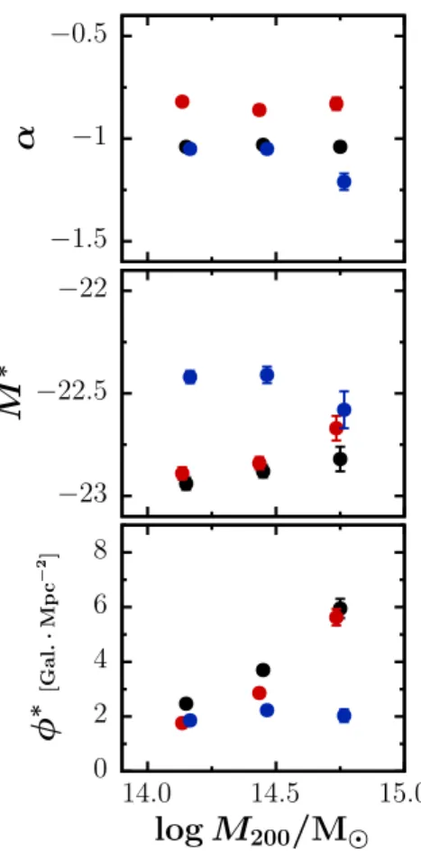
In our three mass bins, the Schechter fits to the GLFs of all the galaxies, of ETGs, and LTGs all converged with a goodness of fit parameter p > 0.72. Using these fits, we study the evolution of the Schechter parameters. Figure 14summarizes the results with each parameter plotted against mass. FigureB.2shows the confidence ellipses on the values of M∗and α.
For the faint-end parameter α, we observe a steepening with increasing mass for the LTG population, from αLTG = −1.05 ±
0.02 for 14 < log (M200) ≤ 14.3 to αLTG = −1.21 ± 0.04 for
log (M200) > 14.6, with a significance of 3.6σ. The ETG
popula-tion and the full galaxy populapopula-tion show no clear evidence for a mass dependence of the faint end. The absolute magnitude char-acteristic parameter M∗is compatible with no mass dependence for the full galaxy population or for the LTGs. For the ETG pop-ulation, M∗decreases with increasing mass with a significance of ∼3σ.
10−3 10−2 10−1 100 101 102 -25 -23 -21 -19 -17 -25 -23 -21 -19 -17 -25 -23 -21 -19 -17 N [Galaxies · Mp c − 2· (0.5 mag) − 1] 1014.0≤ M 200< 1014.3[M ] Nclus = 884 hzi = 0.48 hM200 M i = 1.4 × 10 14 Mabs(i) 1014.3≤ M 200< 1014.6[M ] Nclus = 409 hzi = 0.50 hM200 M i = 2.7 × 10 14 M200> 1014.6[M ] Nclus = 88 hzi = 0.47 hM200 M i = 5.5 × 10 14
Fig. 13.Mass dependence of the i-band stacked GLF in the CFHTLS Wide fields. Black is for all galaxies, red for ETGs, and blue for LTGs. For each figure the number of clusters, their mean redshift, and mass is indicated. The black vertical line indicates the limiting magnitude used in the fit.
−1.5 −1 −0.5 −23 −22.5 −22 0 2 4 6 8 14.0 14.5 15.0
α
M
∗φ
∗ [Gal .· Mp c − 2]log M
200/M
Fig. 14. Dependence of the Schechter fit parameters on mass for all galaxies (black), ETGs (red), and LTGs (blue).
The normalization φ∗depends on mass for the overall galaxy population, with a significance of 9.7σ. This is expected since the normalization of the GLFs is directly related to richness, and richness is a proxy for mass. This is also true for the ETG popula-tion, which shows a clear dependence (with a >12σ significance) meaning that there are more ETGs in massive clusters. On the other hand, the normalization of the GLF of the LTG population seems independent of mass.
6.4. Breaking the degeneracy: GLFs of clusters stacked in mass-redshift bins
When studying a sample of clusters, there is usually a degener-acy between mass and redshift. Indeed, because more massive
clusters are rarer, by binning our clusters in redshift space only we actually sample a population that is more representative of low-mass clusters. However, low-mass clusters are more difficult to detect at high redshift, so the two effects act oppositely and it is difficult to know which one dominates.
To break this degeneracy we need to bin in the 2D parameter space of both mass and redshift. To date this had not been possi-ble because studies of the evolution of cluster GLFs with redshift have been limited to small samples, and extensive studies of the mass dependence concern only low-redshift objects (see e.g.Lan et al. 2016, on SDSS data).
The large size of our cluster candidate catalogue and the depth of the CFHTLS enable us to carry out such an analysis. Indeed, considering the four Wide fields of the CFHTLS, we detect 1371 cluster candidates with M200 > 1014M , S /N > 4
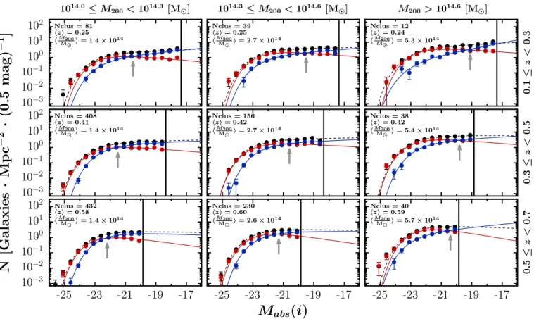
and z < 0.7. Since we computed a robust selection function from the simulations, we know how representative of the true under-lying cluster population our sample is in terms of completeness. Our catalogue is >90% pure in the redshift range considered and at worse ∼50% complete (for the lowest mass and highest red-shift bin). Overall, the 2D bins are well populated, with 12 cluster candidates in the less populated bin and 160 clusters per bin in the mean.
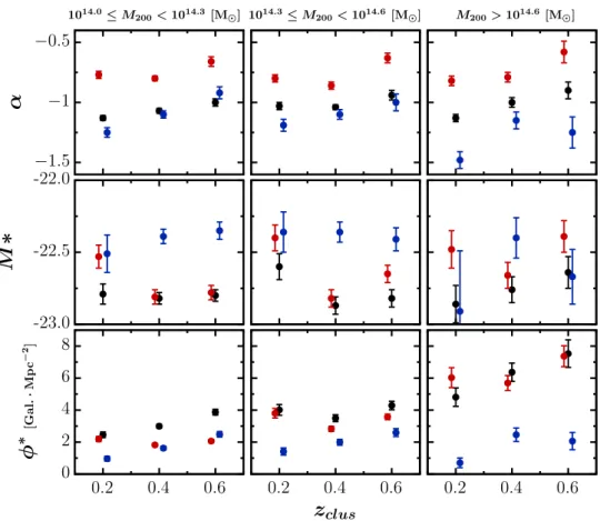
The GLFs obtained in the three redshift bins and three mass bins are shown in Fig.15, where for each panel we indicate the number of cluster candidates stacked, their mean redshift, and mean mass. The best Schechter fit to each galaxy population is overplotted. A grey arrow indicates the absolute magnitude where the red and blue GLFs intersect. We can see that for all cluster masses the intersection moves towards brighter magnitudes as the redshift increases. Therefore the proportion of faint LTGs increases with decreasing redshift. For a given redshift, the grey arrow moves towards fainter magnitudes as the cluster mass increases, implying that in massive clusters the contribution of bright ETGs is higher than in low-mass clusters. At fixed mass, the slope flattens (α more negative) for ETGs and steepens (α more negative) for LTGs from high to low redshift. This leads to the magnitude at which the two populations cross getting brighter at higher redshift. We see the opposite evolution of the slopes with increasing mass compared to the redshift evolution, so that the crossing happens at brighter magnitudes for low-mass clusters.
The best fit parameters are presented in TableC.3, where we also provide the absolute magnitude limit compl to which the fit is performed and the goodness of fit parameter p defined in Eq. (12).