Dynamic bipedal walking assisted by learning

Dynamic Bipedal Walking Assisted by Learning

by

Chee-Meng Chew

B.Eng., Mechanical Engineering

National University of Singapore, 1991

S.M., Mechanical Engineering

Massachusetts Institute of Technology, 1998

Submitted to the Department of Mechanical Engineering

in partial fulfillment of the requirements for the degree of

Doctor of Philosophy in Mechanical Engineering

at the

MASSACHUSETTS INSTITUTE OF TECHNOLOGY

September 2000

@

Chee-Meng Chew, MM. All rights reserved.

The author hereby grants to MIT permission to reproduce and distribute publicly

paper and electronic copies of this thesis documpnt

r

part.

Author ...

...

Department of Mechanical Engineering

August 4, 2000

Certified by ...

Certified by...

...

Gill A. Pratt

Professor of Electrical Engineering and Computer Science

Thesis Supervisor

...

...

Kamal Youcef-Toumi

Professor of Mechanical Engineering

Theis Committee Chair

Accepted by ...

Amn A. Sonin

Chairman, Department Committee on Graduate Students

MASSACHUSETTS INSTITUTE OF TECHNOLOGY

SEP 2 0

2000

LIBRARIES

Dynamic Bipedal Walking Assisted by Learning

by

Chee-Meng Chew

Submitted to the Department of Mechanical Engineering on August 4, 2000, in partial fulfillment of the

requirements for the degree of

Doctor of Philosophy in Mechanical Engineering

Abstract

This thesis proposes a general control architecture for 3D dynamic walking. It is based on a divide-and-conquer approach that is assisted by learning. No dynamic models are required for the implementation.

In the approach, the walking task is divided into three subtasks: 1) to maintain body height; 2) to maintain body posture; and 3) to maintain gait stability. The first two subtasks can be achieved by simple control strategies applied to the stance leg. The third subtask is mainly effected by swing leg behavior. By partitioning the overall motion into three orthogonal planes (sagittal, frontal and transverse), the third subtask can be further divided into forward velocity control (in the sagittal plane) and lateral balance (in the frontal plane). Since there is no explicit solution for these subtasks, reinforcement learning algorithm, in particular, Q-learning with CMAC as function approximator, is used to learn the key parameters of swing leg strategy which determine the gait stability.

Based on the proposed architecture, different control algorithms are constructed and verified using the simulation models of two physical bipedal robots. The simulation analysis demonstrates that by applying an appropriate local control laws at stance ankle joints, the learning rates for the learning algorithms can be tremendously improved.

For the lateral balance, a simple control algorithm (without learning) based on the notion of symmetry is discovered. The stability of the control algorithm is achieved by applying appropriate local control law at the stance ankle joint. A dynamic model is constructed to validate this approach.

The control algorithms are also demonstrated to be general in that they are applicable to different bipeds that have different inertia and length parameters. The designer is also free to choose the walking posture and swing leg strategy. Both "bird-like" and "human-like" walking postures have been successfully implemented for the simulated bipeds.

Thesis Supervisor: Gill A. Pratt

Title: Professor of Electrical Engineering and Computer Science

Acknowledgments

I am indebted to all my lab mates (Jerry Pratt, David Robinson, Dan Paluska, Allen Parseghian, John Hu, Mike Wessler, Peter Dilworth, Robert Ringrose, Hugh Herr, Chris Morse, Ben Krupp, Gregory Huang, Andreas Hoffman) for their contributions to my knowl-edge and awareness in my research area. They were never too tired to answer all my doubts and help me when I ran into problems. I also thank Jerry for designing and building the planar biped "Spring Flamingo". I also thank Jerry, Dave and Dan for designing the three-dimensional biped "M2". These bipeds allowed me to set an application target for my research. I would also like to thank all the present and former lab members who contributed to the design of the simulation package, especially Creature Library, without which my re-search would have been very tedious. I wish to thank my advisor, Professor Gill Pratt, for letting me take on this research. I also wish to thank my other thesis committee members (Professor Youcef-Toumi, Professor Jean-Jacques Slotine and Professor Tomaso Poggio) for coaching me so that I stayed on the right path. I would like to thank Gregory, Andreas, Jerry, Megan and Professor Pratt for proof-reading my thesis. I also wish to thank Professor Leslie Pack Kaelbling and Professor Dimitri P. Bertsekas for answering my questions in the area of reinforcement learning.

I would like to thank all the previous researchers in the biped locomotion for contributing many highly valuable research results based on which I organized my research. I also wish to thank all the researchers in the reinforcement learning field for designing excellent algorithms that can be applied to solve difficult control problems like bipedal walking.

I wish to thank the National University of Singapore because my work at MIT would never have happened without its sponsorship. I also wish to thank my parents, wife (Kris), daughter (En-Chin), and son (Ethan), for being very understanding and for providing me with moral support just at the right moment.

Contents

1 Introduction 13

1.1 Background . . . . 13

1.2 Target Systems . . . . 14

1.3 Objective and Scope . . . . 16

1.4 Approach . . . . 18 1.5 Simulation Tool . . . . 20 1.6 Thesis Contributions . . . . 20 1.7 Thesis Outline . . . . 21 2 Literature Review 23 2.1 Model-based . . . . 23 2.2 Biologically Inspired . . . . 24

2.2.1 Central Pattern Generators (CPG) . . . . 25

2.2.2 Passive Dynamics . . . . 25

2.3 Learning . . . . 26

2.4 Divide-and-conquer . . . . 27

2.5 Summary . . . . 28

3 Proposed Control Architecture 29 3.1 Characteristics of Bipedal Walking . . . . 29

3.2 Desired Performance of Bipedal Walking Task and Control Algorithm . . . 30

3.3 Divide-and-conquer Approach for 3D Dynamic Bipedal Walking . . . . 30

3.3.1 Sagittal Plane . . . . 31

3.3.2 Frontal Plane . . . . 32

3.3.3 Transverse Plane . . . . 32

3.4 Swing Leg Behavior . . . . 32

3.5 Proposed Control Architecture . . . . 33

4 Implementation Tools 35 4.1 Virtual Model Control . . . . 35

4.1.1 Description of Virtual Model Control (VMC) . . . . 35

4.1.2 Application to Bipedal Walking . . . . 36

4.2 Reinforcement Learning . . . . 37

4.2.1 Q-learning . . . . 39

4.2.2 Q-learning Algorithm Using Function Approximator for Q-factors . 42

6 CONT

4.2.3 Other Issues of Reinforcement Learning Implementation . . . . 4.3 Cerebellar Model Articulation Controller (CMAC) . . . .

5 Sagittal Plane Control Algorithms

5.1 Analysis and Heuristics of Sagittal Plane Walking Motion . . . .

5.1.1 Massless Leg Models . . . .

5.1.2 Double-Pendulum Model . . . .

5.2 A lgorithm . . . . 5.2.1 Virtual Model Control Implementation in Sagittal Plane . . . .

5.2.2 Reinforcement Learning to Learn Key Swing Leg Parameter . . . . .

5.3 Effect of Local Speed Control on Learning Rate . . . . 5.4 Generality of Proposed Algorithm . . . . 5.5 Myopic Learning Agent . . . . 5.6 Sum m ary . . . .

6 Three-dimensional walking

6.1 Heuristics of Frontal Plane Motion . . . .

6.2 Frontal and Transverse Planes Algorithms . . . .

6.2.1 Virtual Model Control Implementations in Frontal and Transverse P lan es . . . .

6.2.2 Reinforcement Learning to Learn Key Swing Leg Parameter for Lat-eral B alance . . . .

6.3 Local Control in Frontal Plane . . . . 6.4 Notion of Symmetry . . . . 6.4.1 A nalysis . . . . 6.5 Summary . . . .. . .. 7 Other Implementations 7.1 Variable-Speed Walking . . . . 7.2 Human-like Walking . . . . 8 Conclusions 8.1 Future work . . . . A Transformation Equation

B Image Sequences from Videos

ENTS 43 44 47 47 48 51 56 57 59 63 68 73 75 79 79 80 80 81 83 90 92 99 101 101 102 107 108 111 115

List of Figures

1-1 7-Link 6 DOF planar biped - Spring Flamingo . . . . 15

1-2 Three-dimensional biped: M2 (CAD drawing by Daniel Paluska) . . . . 15

1-3 The orthogonal planes: Sagittal, Frontal and Transverse. . . . . 19

3-1 Proposed control architecture . . . . 34

4-1 A possible set of virtual components to achieve walking control for Spring F lam ingo . . . . 37

4-2 Q-learning algorithm based on lookup table[115, 102] . . . . 40

4-3 Q-learning algorithm using CMAC to represent Q-factors . . . . 43

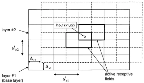
4-4 Schematic diagram of CMAC implementation . . . . 45

4-5 An addressing scheme for a two-dimensional input CMAC implementation . 46 5-1 Massless leg model: Inverted pendulum. 0 is the angle measured from the vertical, g is the gravitational constant, and 1 is the leg length. . . . . 49

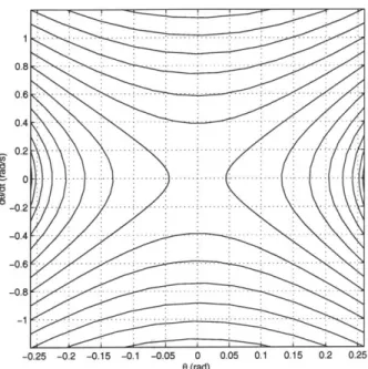
5-2 Phase diagram of the inverted pendulum model. Each contour corresponds to a specific energy level for the system. . . . . 50

5-3 Massless leg model: Linear inverted pendulum. x is the horizontal coordinate of the point mass from the vertical plane that passes through the ankle joint. 50 5-4 An Acrobot model is adopted for the single support phase of the bipedal walking in the sagittal plane. It has two point masses M and m that rep-resents the body and swing leg inertia, respectively. It is actuated only at the joint between the two links. The joint that is attached to the ground is assumed to have zero torque. . . . . 53

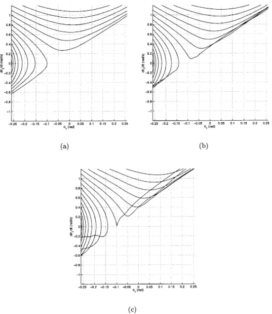
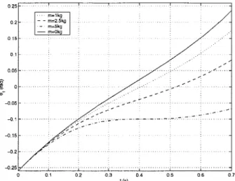
5-5 Phase portraits of the stance leg's angular position and velocity (based on the Acrobot model). The swing leg is commanded to travel from 02 = -150' to -210' in 0.7 second based on a third degree polynomial function of time (with zero start and end values for 92): (a) m = 1kg; (b) m = 2.5kg; and (c) m=5kg. ... ... ₅₄

5-6 Trajectories of the stance leg angular position

01

01

LIST OF FIGURES

5-7 Effect of controller dynamics on the trajectory of the stance leg angular position 01. The swing leg is commanded to travel from 02 = -1500 to -210"

in 0.7 second as before. The solid curve corresponds to the PD controller with the proportional gain set at 2000Nm and the derivative gain set at 200Nms. The dashed curve corresponds to the PD controller with the proportional gain set at 200Nm and the derivative gain set at 20Nms. . . . . 56 5-8 Finite state machine for the bipedal walking control algorithm. . . . . 58

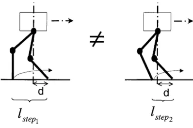
5-9 Two postures of the biped when the swing foot touches down. Though x (x-coordinate of the previous swing ankle measured with reference to the hip when the swing leg touches down) is the same (= d) for both postures, the

step lengths (1step, and lsteP2) are different. If the dynamics of the swing leg

is not ignorable, the next swing leg dynamics for both postures will have different effects on the body motion. . . . . 61 5-10 Schematic diagram of the RL implementation for the sagittal plane. '+ is

the velocity of the hip in the x-direction; xta is the x-coordinate of the swing ankle measured with reference to the hip; 1+ is the step length. Superscript

+

5-11 A local speed control mechanism based on stance ankle joint. . . . . 63 5-12 The graphs show that the local control based on the stance ankle increases the

learning rate. The dashdot-line graph corresponds to the simulation result with the local control at the ankle. The solid-line graph is without the local control. In both cases, the starting posture (standing posture) and the initial speed (0.4m/s) are the same for each training iteration. . . . . 66 5-13 The graphs show the action (Xha) sequences generated by the learning agent

(with local control at the stance ankle) for the 1st, 5th, 1 0th, 1 5th and 1 6th

learning iterations. The corresponding forward velocity

(i)

posture (standing posture) and the initial speed (0.4m/s) are the same for each training iteration. . . . . 67 5-14 The learning curves of the simulated Spring Flamingo correspond to different

swing times (0.2, 0.3, 0.4 and 0.5 second). The local control based on the stance ankle is used. The starting posture (standing posture) and the initial speed (Om/s) for each training iteration are the same for all the cases. . . . 68

5-15 For a given foot placement location, different swing times yield different

postures at the end of the step. . . . . 69

5-16 Learning curves for the simulated M2 (constrained to the sagittal plane) and

Spring Flamingo (using implementation S_2). . . . . 71 5-17 Stick diagram of the dynamic walking of the simulated Spring Flamingo after

the learning target was achieved (using implementation 52). Only the left leg is shown in the diagram, and the images are 0.1 second apart. . . . . 71

5-18 The simulation data for the dynamic walking of the simulated Spring Flamingo

after the learning target was achieved (using implementation S-2). . . . . . 72 8

LIST OF FIGURES

5-19 V denotes the hip velocity when the vertical projection of the biped's center

of mass passes through the stance ankle. This value is used to evaluate the action taken for the swing leg. . . . . 73 5-20 A learning curve for the simulated M2 (constrained to the sagittal plane)

when implementation S_3 was used. . . . . 76 5-21 The simulation data for the dynamic walking of the simulated M2

(con-strained to the sagittal plane) after the learning target was achieved (using im plem entation S_3). . . . . 77

6-1 State variables for the learning implementation in the frontal plane motion are the values of y,

#

inverted pendulum model. The black circle represents the point mass of the linear inverted pendulum model. . . . . 84

6-3 The learning curves for the simulated M2 when implementations F_1 and S_4 were used. The learning in both the sagittal and frontal planes was carried out simultaneously. The solid-line and dotted-line graphs are the learning curves for the implementations in which the frontal plane's local controls were based on Equations 6.5 and 6.8, respectively. The implementa-tion whose frontal plane's local control was based on Equaimplementa-tion 6.8 managed to achieve the learning target in about 200 learning iterations. The other implementation did not seem to improve its walking time even after around

600 learning iterations. . . . . 88

6-4 The simulation data (after the simulated M2 has achieved the learning target) for the implementation F_1 whose local control is based on Equation 6.8 . . 89 6-5 A learning curve for the dynamic walking of the simulated M2. The frontal

plane implementation was based on the notion of symmetry. The sagittal plane implementation was SA4. . . . . 92 6-6 Stick diagram of the dynamic walking of the simulated M2 after the learning

target was achieved. Only the left leg is shown in the diagram and the images are 0.1 second apart. . . . . 93 6-7 The body trajectory of M2 during the dynamic walking after the learning

target was achieved. The frontal plane implementation was based on the notion of symmetry. The sagittal plane implementation was SA4. . . . . 94

6-8 The legs' roll angle trajectories of M2 during the dynamic walking. The frontal plane implementation was based on the notion of symmetry. The sagittal plane implementation was S_4. The present step length 1+ and action sequences of the sagittal plane implementation are also included. . 95

6-9 A linear double pendulum model for the analysis of the symmetry approach

used in the frontal plane algorithm. . . . . 96 6-10 Four surface plots of the maximum modulus of the eigenvalues of H against

Kp and KD corresponding to K1 = 1, 10, 20 and 50. . . . . 98

7-1 A learning curve for the variable-speed walking implementation. . . . .1 9

LIST OF FIGURES

7-2 The body trajectory and selected output variables of the simulated M2 during the variable-speed walking. . . . . 104

7-3 Mechanical limit is used to prevent the legs from hyper-extension in human-like walking simulations. . . . . 105

7-4 A learning curve for the human-like walking implementation. . . . . 106 7-5 Stick diagram of the "human-like" walking of the simulated M2. Only the

left leg is shown in the diagram and the images are 0.05 second apart. . . . 106

A-1 A planar four-link, three-joint model which is used to represent the stance

leg of the bipedal robot. Coordinate frame

{B}

B-1 The rear view image sequence (left to right, top to bottom) of the 3D bird-like walking implementation of the simulated M2. The control algorithm and implementation parameters can be found in Section 6.4. The images are 0.13s apart. . . . . 116 B-2 The side view image sequence (left to right, top to bottom) of the 3D

bird-like walking implementation of the simulated M2. The control algorithm and implementation parameters can be found in Section 6.4. The images are 0.13s apart. . . . .. . 117 B-3 The side view image sequence (left to right, top to bottom) of the 3D

human-like walking implementation of the simulated M2. The control algorithm and implementation parameters can be found in Section 7.2. The images are 0.1s ap art. . . . . 118

List of Tables

1.1 Specifications of Spring Flamingo . . . . 16

1.2 Specifications of M 2 . . . . 17

5.1 Description of the states used in the bipedal walking control algorithm . . . 57

5.2 Parameters of the virtual components for the stance leg (in the sagittal plane). 58 5.3 Reinforcement learning implementation for the sagittal plane: S_1 . . . . . 65

5.4 Reinforcement learning implementation for the sagittal plane: S_2 . . . . . 70

5.5 Reinforcement learning implementation for the sagittal plane: S_3 . . . . . 74

5.6 Summary of the sagittal plane implementations . . . . 78

6.1 Reinforcement learning implementation for the frontal plane: F_1 . . . . 86

6.2 Reinforcement learning implementation for the sagittal plane: S4 . . . . . 87

Chapter 1

Introduction

1.1

Background

Animal locomotion research has been around for more than a century. As defined by Inman, Ralston and Todd [41]: "Locomotion, a characteristic of animals, is the process by which animal moves itself from one geographic position to another. Locomotion includes starting, stopping, changes in speed, alterations in direction, and modifications for changes in slope." Bipedal locomotion is associated with animals that use exactly two limbs to achieve locomotion. There are numerous reasons for studying bipedal locomotion and building bipedal robots. The main motivation is that human beings are bipedal. It is desirable for us to replicate a machine with the same mobility as ourselves so that it can be placed in human environments, especially in areas that pose great hazard for human beings.

It is also interesting to understand the basic strategies of how bipedal creatures perform walking or running. It is interesting to find out why the walking task, which can be easily performed by human beings and other living bipeds, seems to be daunting for a robotic biped. This understanding may aid the development of better leg prostheses and help many people who lose their lower extremities walk again. It may also be applied to rehabilitation therapy for those who lose their walking ability.

It is a great challenge for scientists and engineers to build a bipedal robot that has agility and mobility similar to a human. The complexity of bipedal robot control is mainly due to the nonlinear dynamics, unknown environment interaction, and limited torque at the stance ankle (due to the fact that the feet are not fixed to the ground).

Many algorithms have been proposed for the bipedal walking task [71, 25, 36, 32, 7, 43,

38, 39, 40, 52, 50, 55, 28, 70, 31]. To reduce the complexity of the bipedal walking analysis,

some of the researchers restricted themselves to planar motion studies, some adopted simple models or linearization approaches, etc. Waseda University [106, 107, 122, 123] has con-ducted much research on 3D bipedal walking. All the implementations adopt a stabilization approach using trunk motion. The algorithms derived are thus not applicable to a biped that does not have the extra DOF on the body.

Honda humanoid robots (P2 and P3) [38] are the state-of-the-art 3D bipedal walking systems. They do not have extra DOF on the body to provide the stabilization control as in Waseda's robots. The lower extremities have the minimum number of DOF (6 DOF in each leg) which still allow the same mobility as human beings. Thus, the robots are capable

CHAPTER 1. INTRODUCTION

of achieving most walking behaviors of their human counterparts.

Honda's control method is based on playing back trajectory recordings of human walk-ing on different terrains [78]. Though the resultwalk-ing walkwalk-ing execution is very impressive, such a reverse engineering approach requires iterative parameter tunings and tedious data adaptation. These are due to the fundamental differences between the robots and their human counterparts, for example, the actuator behaviors, inertias, dimensions, etc.

The MIT Leg Laboratory has recently designed and built a 3D bipedal robot called M2 (see Section 1.2). The robot has the same DOF at the lower extremities as the Honda's robots. Apart from the approach by Honda, there are very few algorithms proposed for such a biped. In this thesis, the author aims to construct and investigate new 3D dynamic walking algorithms for the biped.

1.2

Target Systems

For legged robots, the control algorithms are very much dependent on the structure, degrees of freedom, actuator's characteristics of the robot. This section describes the bipedal robots for which the walking control algorithms are designed.

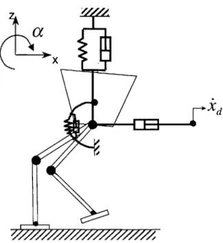
Two bipedal robots will be considered in this thesis. One is a headless and armless 7-link planar bipedal robot called Spring Flamingo (see Figure 1-1). It is constrained to move in the sagittal plane. The legs are much lighter than the body. Each leg has three actuated rotary joints. The joint axes are perpendicular to the sagittal plane. The total weight is about 12 kg.

The biped has a rotary angular position sensor at each DOF. It is used to measure the relative (anatomical) angular position between consecutive links. In the simulation model, it is assumed that the biped has a single axis gyrocope or an inclinometer fixed to the body which can provide the body posture information '. Each foot has two contact sensors at the bottom, one at the heel and one at the toe, to determine ground contact events.

The other robot is an unconstrained (3D) biped called M2 (Figure 1-2). It is also headless and armless. However, it has more massive legs compared with Spring Flamingo. Each leg has six active DOF of which three DOF is available at the hip (yaw, roll, pitch), one at the knee (pitch) and two at the ankle joint (pitch, roll). Each DOF has an angular position sensor to measure the relative angle between two adjacent links. Each of the feet has four force sensors (two at the toe and two at the heel) to provide the contact forces between the feet and the ground. A gyroscopic attitude sensor is mounted in the body to detect its roll, pitch and yaw angles. The total weight is about 25kg.

In both systems, the joints are driven by force/torque controlled actuators called Series Elastic Actuators [79]. The dynamic range of the actuators is quite good, and they are assumed to be force/torque sources in the simulation analysis in this thesis. Simulation models of these robots are created using the simulation tool described in Section 1.5. The model specifications for Spring Flamingo and M2 are given in Table 1.1 and 1.2, respectively.

'In the real robot, the body posture is provided by an angular position sensor attached between the body and a boom.

1.2. TARGET SYSTEMS Ii, --- m3,I 1,3 M2, 2 1c2 12 m1,11 "F- 0x

(a)

(b)

Figure 1-1: 7-Link 6 DOF planar biped - Spring Flamingo

'a

pitch

ya w it y

ro x

(b)

Figure 1-2: Three-dimensional biped: M2 (CAD drawing by Daniel Paluska)

(a)

CHAPTER 1. INTRODUCTION

Table 1.1: Specifications of Spring Flamingo

1.3

Objective and Scope

In terms of walking gaits, bipedal locomotion research can be classified into two main areas: 1) static walking and 2) dynamic walking. In static walking, the biped has to move very slowly so that its dynamics can be ignored. A static walking algorithm usually tries to maintain the biped's projected center of gravity (PCOG) within the boundary of the supporting foot or the smallest convex hull containing the two feet during the double support phase. By obeying this constraint and walking sufficiently slowly, the biped would not fall over if it freezes all its joints at any instance. Static walking is simple to implement because only geometry information is required to compute the location of the projected center of gravity. However, the walking speed and step size are limited.

In dynamic walking, the motion is faster and hence, the dynamics are not negligible.

If the biped suddenly freezes all its joints, its momentum may cause it to topple over. In

dynamic walking, one can look at the zero moment point (ZMP) [112] rather than PCOG. The ZMP is the point where the resulting reaction moment vector on the foot does not have a component in the horizontal plane (assuming the foot is on a horizontal ground). However, the ZMP does not have direct implications for walking stability. The choice of an appropriate and alternating sequence of steps between left and right leg results in walking stability. Dynamic walking usually results in larger step lengths and greater efficiency than static walking. However, the stability margin of dynamic walking is much harder to quantify. The objective of this thesis is to synthesize and investigate a general control architecture for M2, or other robots that have the same DOF, to achieve 3D dynamic bipedal walking. In subsequent chapters, the walking task refers to the dynamic case unless otherwise specified. The control architecture is based on a divide-and-conquer approach in which the 3D bipedal walking task is decomposed into smaller subtasks. A learning method is applied to those

Description Value Total Mass 12.04kg Body Mass 10.00kg Thigh Mass 0.46kg Shin Mass 0.31kg Foot Mass 0.25kg

Body's Moment of Inertia about COM 0.100kgm2

Thigh's Moment of Inertia about 0.0125kgm2

COM

Shin's Moment of Inertia about COM 0.00949kgm2

Foot's Moment of Inertia about COM 0.00134kgm2

Thigh Length 0.42m

Shin Length 0.42m

Ankle Height 0.04m

Foot Length 0.15m

1.3. OBJECTIVE AND SCOPE Table 1.2: Specifications of M2 Description Value Total Mass 25.00kg Body Mass 12.82kg Thigh Mass 2.74kg Shin Mass 2.69kg Foot Mass 0.66kg

Body's Principal Moment of Inertia

x-axis 0.230kgm2

y-axis 0.230kgm2

z-axis 0.206kgm2

Thigh's Principal Moment of Inertia

x-axis 0.0443kgm2

y-axis 0.0443kgm2

z-axis 0.00356kgm2

Shin's Principal Moment of Inertia

x-axis 0.0542kgm2

y-axis 0.0542kgm2

z-axis 0.00346kgm 2

Foot's Principal Moment of Inertia

x-axis 0.000363kgm2 y-axis 0.00152kgm2 z-axis 0.00170kgm2 Hip Spacing 0.184m Thigh Length 0.432m Shin Length 0.432m

Ankle Height (from ankle's pitch axis) 0.0764m

Foot Length 0.20m

Foot Width 0.089m

CHAPTER 1. INTRODUCTION

subtasks that do not have simple solutions. Besides being able to achieve a stable walking gait, the resulting algorithm should achieve the following walking specifications:

1. The biped should be able to walk even when the step length is constrained.

2. The biped should be able to vary the walking speed.

The control algorithm should also have the following characteristics:

1. It should be easy to implement.

2. It should be applicable for real-time implementation.

3. It should be applicable to bipeds of different mass and length parameters.

4. The learning rate of the learning component to achieve the learning target should be

high.

These specifications will be discussed in more detail in Section 3.2. The scope of this research is restricted to bipedal walking on level ground along a linear path. The analysis will be carried out in a dynamic simulation environment. Only the transient behavior from standing to forward walking is included in the analysis. The transient from walking to standing will not be studied though it should be achievable by the proposed approach. This thesis will also not study other behaviors of bipeds like static walking, turning, jumping, running, etc.

1.4

Approach

This section briefly explains how the specifications presented in the previous section can be achieved or implemented. The key philosophy adopted in this thesis is to seek the simplest possible control algorithm that satisfies the specifications stated in Section 1.3. The reason for such a guideline is that bipedal walking is usually very complex (especially dynamic walking). Therefore, it is not advisable to adopt very complex control algorithms. Otherwise, the overall system is most likely to be extremely complex or even intractable.

One of the ways to reduce the complexity of the problem is by task decomposition or divide-and-conquer approach. For example, 3D bipedal walking can be broken down into motion controls in the transverse, sagittal and frontal planes (see Figure 1-3). Each of these can then be considered individually.

Pratt et al. [80] proposed an intuitive control algorithm called "Turkey Walking" for planar bipedal walking based on a control language called Virtual Model Control. In the algorithm, the planar walking task is decomposed into three subtasks: 1) to maintain body height; 2) to maintain body speed; and 3) to maintain body posture.

The algorithm is well behaved and can easily be extended for rough terrain locomotion [20]. However, the control mechanism for the body speed can only be applied during the double support phase. It requires the double support phase to be significant in order to do the job. This requires the swing leg to be swung rapidly so as to produce longer period of the double support phase. This is hard to achieve when the walking speed is high because the real robot usually has limited joint torques. Furthermore, fast swing-leg motion consumes

1.4. APPROACH

.-

Frontal Plane

Transverse Plane

Figure 1-3: The orthogonal planes: Sagittal, Frontal and Transverse.

more energy. Due to the deficiency of the speed control based on the double support phase, this thesis does not adopt this strategy. Instead, the swing leg behavior is considered to be the key determinant for the gait stability. This idea is applicable to both forward speed stabilization and lateral balance of bipeds. However, due to the complexity of the bipedal walking sytem, there is no closed form expression for the foot placement parameters in terms of the desired walking speed or other gait parameters. As such, a learning approach is proposed for the swing leg task.

In this thesis, the divide-and-conquer approach used in the "Turkey Walking" algorithm is extended to the 3D walking task. In the 3D walking task, the motion control is first par-titioned into the three orthogonal planes. Each of these is further subdivided into smaller subtasks. A learning algorithm is used to assist those subtasks that are not easily accom-plished by simple strategies or control laws. The overall control algorithm should satisfy the desired performance specifications discussed before.

In this approach, the learning time is expected to be shorter than those learning ap-proaches that learn all the joint trajectories from scratch. This is because the scope of learning is smaller and less complex if the learning algorithm focuses on just a subtask. Furthermore, the previous research results of the Turkey Walking algorithm can be uti-lized. In summary, the robot should only learn the tasks or parameters that really require learning. A detailed description of this approach is presented in Chapter 3.

19

Sagittal Plane

CHAPTER 1. INTRODUCTION

1.5

Simulation Tool

SD FAST, a commercial dynamic simulation program from Symbolic Dynamics, Inc [91] is used to generate the dynamics of the simulated bipeds. It is based on Newtonian mechanics for interconnected rigid bodies. An in-house simulation package called the Creature Library [88] is used to generate all the peripheral C routines (except for the dynamics) for the simulation after a high level specification of the biped is given.

The dynamic interaction between the biped and the terrain is established by specifying four ground contact points (two at the heel and two at the toe) beneath each of the feet. The ground contacts are modeled using three orthogonal spring-damper pairs. If a contact point is below the terrain surface, the contact model will be activated and appropriate contact force will be generated based on the parameters and the currect deflection of the ground contact model. If a contact point is above the terrain surface, the contact force is zero.

Before a simulation is run, the user needs to add a control algorithm to one of the C programs. In the control algorithm, only information that is available to the physical robot is used. The body orientation in terms of the roll, pitch, yaw angles and the respective angular velocities are assumed to be directly available. All the joint angles and angular velocities are also known. The contact points at the foot provide information about whether they are in contact with the ground or not.

The output of the control algorithm is all the desired joint torques. The dynamics of the actuators are ignored in the simulation. That is, the actuators are considered to be perfect torque or force sources.

1.6

Thesis Contributions

The contributions of this thesis are:

1. The synthesis of a general control architecture for 3D dynamic bipedal walking based on a divide-and-conquer approach. Learning is applied to achieve gait stability. No prior mathematical model is needed.

2. The demonstration that dynamic walking can be achieved by merely learning param-eters of swing leg control.

3. The design and investigation of several walking algorithms based on the proposed control architecture.

4. The demonstration of the effects of local control mechanism on learning rate and stabilization.

5. The application of the notion of symmetry for lateral balance during forward walking. A quantitative analysis has been done to verify the approach.

6. The demonstration of the generality of the control architecture by applying the al-gorithm to different bipeds that have similar degrees of freedom but different inertia and length parameters.

1.7. THESIS OUTLINE

1.7

Thesis Outline

Chapter two gives a literature review of the bipedal locomotion research that is relevant

to this thesis. It groups bipedal walking research into four categories. Examples of each of the categories are discussed.

Chapter three presents the common characteristics of bipedal walking. It also

de-scribes the desired performance of the walking task and the control algorithm. The moti-vation for the approach adopted in this thesis is then discussed. A control architecture for

the 3D dynamic walking task is presented.

Chapter four describes the methods or tools utilized to formulate the walking control

algorithm based on the proposed control architecture. It includes Virtual Model Control which is used to facilitate the transformation of the desired behavior of the stance and swing legs into respective joint torques. It also describes a reinforcement learning method called Q-learning that is used to learn the key swing leg parameters.

Chapter five first presents an analysis of the sagittal plane walking motion. The swing

leg dynamics is demonstrated to be significant and not ignorable in general based on a simple double pendulum model. The application of learning to the control algorithm is also justified. After that, several algorithms for the sagittal plane walking are presented. The usage of the local control at the stance ankle joint in speeding up the learning process is illustrated by simulations. The generality of the proposed control architecture is also demonstrated by applying one of the algorithms to two different bipeds.

Chapter six first presents some heuristics of the frontal plane motion. Then, the frontal

and transverse planes algorithms are presented. They are combined with the sagittal plane to form a 3D dynamic walking algorithm. Two approaches for the lateral balance are highlighted. One is based on the learning approach and the other is based on the notion of symmetry. A simple model is constructed to verify the latter approach. All the algorithms are verified in the simulation environment using the simulated M2.

Chapter seven includes two other implementations to illustrate the flexibility and

generality of the proposed control architecture. One of these is the variable walking speed implementation. The other is to achieve a different walking posture.

Chapter eight concludes the work of this thesis and suggests future work.

Chapter 2

Literature Review

Much research has been done in the area of bipedal locomotion in recent years. Since bipedal locomotion is a complex problem and the scope of bipedal locomotion is wide, most researchers have restricted their research to a smaller area. For example, some researchers have concentrated on the area of mechanics, some on control, some on energetics of biped locomotion, etc. Some researchers further simplify matters by partitioning the biped gait and restricting their analysis either to the sagittal plane or the frontal plane.

For a biped robot to achieve a walking gait, the control algorithm needs to comply with the constraints of the bipedal system. One important constraint is the unpowered DOF between the foot and the ground [112]. This constraint limits the trajectory tracking approach used commonly in manipulator research and is one of the main reasons bipedal locomotion is such a challenging research area.

This chapter classifies the control approaches adopted for dynamic bipedal walking into four categories: 1) model-based; 2) biologically inspired; 3) learning; and 4) divide-and-conquer. Various approaches for each of the categories will be presented. These classes of approach discussed in this chaper are by no means mutually exclusive or complete. Some research may combine several of these approaches when designing a control algorithm for the bipedal walking.

2.1

Model-based

In this approach, a mathematical model of the biped derived from physics is used for the control algorithm synthesis. There is a spectrum of complexity for a biped model, ranging from a simple massless leg model to a full model which includes all the inertial terms, friction, link flexibility, actuator dynamics, etc. Except for certain massless leg models, most biped models are nonlinear and do not have analytical solutions. In addition, there is underactuation between the stance foot and the ground; and unknown discrete changes in the state due to foot impact.

The massless leg model is the simplest model for characterizing the behaviors of the biped. The body of the biped is usually assumed to be a point mass and can be viewed to be an inverted pendulum with discrete changes in the support point. The massless leg model is applicable mainly to a biped that has small leg inertia with respect to the body.

CHAPTER 2. LITERATURE REVIEW

In this case, the swing leg dynamics can be ignored under low walking speed.

Kajita et al. [52, 50] have derived a massless leg model for a planar biped that follows a linear motion. During single support phase, the resulting motion of the model is like a point mass inverted pendulum with variable length. The dynamic equations of the resulting linear motion can be solved analytically. From the model, the touchdown condition of the swing foot is determined based on an energy parameter. Inverse kinematics is used to specify the desired joint trajectories and simple control law is used at each joint for tracking.

When the leg inertia is not ignorable, it needs to be included in the biped model. One basic model that includes the leg inertia is the Acrobot model [118, 73]. It is a double pendulum model with no actuation between the ground and the base link (corresponding to the stance leg). This is commonly used to characterize the single support motion of the biped.

When the leg inertia and other dynamics like that of the actuator, joint friction, etc are included, the overall dynamic equations can be very nonlinear and complex. A linearization approach is usually adopted to simplify these dynamic equations. The linearization can be done with respect to selected equilibrium points to yield sets of linearized equations.

Miura and Shimoyama [71] built a 3D walking biped that had three links and three actuated degrees of freedom: one at each of the hip roll joints and one for fore and aft motion of the legs. The ankle joints were limp. The biped was controlled using a linearized dynamic model. The model assumed that the motions about the roll, pitch and yaw axes were independent. It also assumed that the yaw motion was negligible and there was no slipping between the feet and the ground. After selecting a set of feasible trajectories for the joints, state feedback control laws were then formulated for the joints to generate compensating inputs for the nominal control inputs. The control laws ensured the convergence of the actual trajectories to the desired trajectories. Since they adopted a linearized model for the biped, the motion space had to be constrained to a smaller one so that the model was not violated.

Mita et al. [70] proposed a control method for a planar seven-link biped (CW-1) using a linear optimal state feedback regulator. The model of the biped was linearized about a commanded attitude. Linear state feedback control was used to stabilize the system based on a performance function so that the biped did not deviate from the commanded attitude. For the gait control, three commanded attitudes were given within a gait interval and the biped could walk arbitrary steps with one second period. They assumed that the biped had no torque limitation at the stance ankle. The biped had large feet so that this assumption was valid.

2.2

Biologically Inspired

Since none of the bipedal robots match biological bipeds in terms of mobility, adaptability, and stability, many researchers try to examine biological bipeds so as to extract certain algorithms (reverse engineering) that are applicable to the robots.

The steps taken are usually as follows. First, the behaviors of the biological system are observed and analyzed. Then, mathematical models and hypotheses for the behaviors are proposed. After that, they are verified through simulations or experiments. However, in

2.2. BIOLOGICALLY INSPIRED

most cases, the observations only constitute a small piece of the big puzzle. Thus, their applications to the bipedal robots can be limited.

This subsection includes two main research areas in this category. The first is the Central Pattern Generators (CPG) approach which is based on the findings that certain legged animals seem to centrally coordinate the muscles without using the brain. The second is the passive walking approach that is based on the observation that human beings do not need high muscle activities to walk.

2.2.1 Central Pattern Generators (CPG)

Grillner [34] found from experiments on cats that the spinal cord generated the required signal for the muscles to perform coordinated walking motion. The existence of a central pattern generator that is a network of neurons in the spinal cord was hypothesized.

The idea of CPG was adopted by several researchers for bipedal walking [103, 104, 7]. One typical approach is the use of a system of coupled nonlinear equations to generate signals for the joint trajectories of bipeds. The biped is expected to achieve a stable limit cycle walking pattern with these equations.

Taga [103, 104] applied a neural rhythm generator to a model of human locomotion. The neural rhythm generator was composed of neural oscillators (a system of coupled nonlinear equations) which received sensory information from the system and output motor signals to the system. Based on simulation analysis, it was found that a stable limit cycle of locomotion could emerge by the principle of global entrainment. The global entrainment was the result of the interaction among the musculo-skeletal system, the neural system and the ground.

Bay and Hemami [7] demonstrated that a system of coupled van der Pol oscillators could generate periodic signals. The periodic signals were then applied to the walking task to produce rhythmic locomotion. In their analysis, the dynamics of the biped such as the force interactions between the support leg(s) and the ground were not considered.

One disadvantage of a CPG approach based on a set of coupled nonlinear equations is that there are many parameters to be tuned. It is also difficult to find a set of parameters that enable entrainment of the overall system. Even if a periodic walking behavior can be obtained, it is hard to predict the walking behavior when it is subjected to disturbance due to uncertain ground profile. It is also hard to change the behavior or add more behaviors.

2.2.2 Passive Dynamics

Passive dynamics study provides interesting natural dynamic model for the mechanics of human walking [63, 64, 30]. It was partly inspired by a bipedal toy that was capable of walking down a slope without any actuator system. The toy rocked left and right in a periodic motion. When a leg is lifted in the process, it could swing freely forward and arrived in a forward position to support the toy for the next half period of the motion. If the slope is within a certain range, a stable limit cycle behavior can be observed. When this occurs, the work done on the toy by the gravitational force equals the energy loss by the biped (e.g., impact loss, friction at the joints between the body and the legs).

Most passive dynamics analyses study the stability and periodicity issue of passive walk-ing. Similar to the bipedal toy, most passive walking implementations do not incorporate

CHAPTER 2. LITERATURE REVIEW

any actuator systems or active controllers in the walker. The walking behaviors are usually demonstrated on a downslope so that the gravitational potential energy can be utilized to generate the walking motion.

Though passive walking has nice properties like being able to achieve a minimum energy gait without active control, it is sensitive to parameter variations [63], such as, the mass distribution, joint friction etc. During physical implementation, iterative tuning is usually required before a successful implementation can be achieved. Furthermore, it is still unclear how it can be implemented for rough terrain walking.

2.3

Learning

The learning approach is often touted to possess biological behaviors. It is evident from observing toddlers who are just starting to walk that walking is a learned process. Learning is also commonly applied to systems whose models are hard to derive or implement. In some cases, learning is used to modify a nominal behaviors that are generated based on a

simplified model.

Miller, Latham and Scalera [69] adopted a simple gait oscillator which generates the trajectory of the swing leg for a simulated planar biped. The input to the oscillator was the step time and the desired step length based on a fixed model. A CMAC (Cerebellar Model Articulation Controller) network was used to adjust the desired step length based on past experience. The purpose was to achieve a desired forward velocity at the end of each step. The CMAC network was trained under two different times scales. Based on the velocity error at the end of each step, a supervised learning approach was adopted to adjust the step length prediction of the last control cycle of the previous step. Also, the step length prediction for each control cycle was adjusted based on the prediction in the next control cycle. When the biped fell forward or backward during a step, the CMAC network step length prediction at the end of the last step was adjusted by a fixed value in a direction opposite to the fall direction. The control algorithm was successfully implemented for a simulated planar three-link biped with massless legs.

Wang, Lee, and Gruver [113] presented a neuromorphic architecture based on supervised learning for the control of a three-link planar biped robot. Based on the biped's dynamic model, a control law was obtained by nonlinear feedback decoupling and optimal tracking approach. Then, they used a hierarchical structure of neural networks to learn the control law when the latter was controlling the biped. They assumed that the desired joint trajec-tories were available. However, in physical implementation, due to the torque limitation of the stance ankle, it is difficult to obtain a working set of joint trajectories without violating this constraint.

Miller [66] designed a learning system using neural networks for a biped that was capable of learning the balance for side-to-side and front-to-back motion. With the help of several control strategies, the neural networks learn to provide feedforward control to the joints. The biped had a slow walking gait after training.

Benbrahim and Franklin [9] applied reinforcement learning for a planar biped to achieve dynamic walking. They adopted a "melting pot" and modular approach in which a central controller used the experience of other peripheral controllers to learn an average control policy. The central controller was pre-trained to provide nominal trajectories to the joints.

2.4. DIVIDE-AND-CONQUER

Peripheral controllers helped the central controller to adapt to any discrepancy during the actual run. The central controller and some of the peripheral controllers used simple neural networks for information storage. No dynamic model of the system was required in the implementation. One disadvantage of the approach was that the nominal joint trajectories were required to train the central controller before any learning began. This information is usually not easily obtainable.

In summary, there are many ways to implement a learning algorithm for the biped. It depends not only on the level of the control hierarchy to which learning is applied but also on how the control task is decomposed. Of course, the design of the bipedal robot also greatly influences the algorithm, especially the actuator and sensor systems and the degrees of freedom. Furthermore, just as in any optimization techniques, learning success relies very much on the performance index chosen.

2.4

Divide-and-conquer

Due to the complexity of the bipedal walking system, many implementations break the problem into smaller sub-problems that can be solved more easily. Intuition of the problem is usually required for such an approach, both in deciding how to break down the problem and how to solve the smaller sub-problems. Intuition can be obtained by observing the behavior of bipedal animals (similar to the biologically inspired approach), by analyzing simple dynamic models, etc.

Raibert's control algorithms [86] for hopping and running machines mostly utilized the divide-and-conquer approach. For example, the control algorithm for a planar one-legged hopping machine was decomposed into: 1) the hopping motion (vertical); 2) forward motion (horizontal) and; 3) body posture. These sub-tasks were considered separately and each was implemented using simple algorithm. This resulted in a simple set of algorithms for the hopping task.

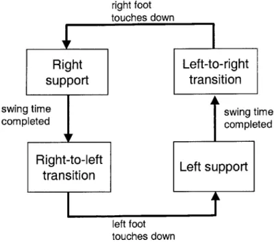
Pratt et al. [81, 80] presented a control algorithm (called "Turkey Walking") based on a divide-and-conquer approach for planar bipedal walking task of a biped called "Spring Turkey". The walking cycle was first partitioned into two main phases: double support and single support. A simple finite state machine was used to keep track of the currently active phase. In the double support phase, the task of the controller consisted of three sub-tasks:

1) body pitch control; 2) height control and; 3) forward speed control. In the single support

phase, the task of the controller consisted of two sub-tasks: 1) body pitch control and 2) height control. Based on this framework, a control language called Virtual Model Control (VMC) was used to design the control algorithm. The resulting algorithm was simple and low in computation since no dynamic equations were used. It was successfully implemented to control a planar biped for dynamic walking on level ground in real-time. Chew [18] has extended the algorithm for rough terrain locomotion.

The divide-and-conquer approach has been proven to be simple and effective for practical implementations. However, not all the sub-tasks contain direct or analytic solutions. Some may require tedious iterative parameter tunings.

CHAPTER 2. LITERATURE REVIEW

2.5

Summary

This chapter gives a classification of the research on dynamic bipedal walking. It is by no means complete. Many excellent studies were omitted to keep this chapter concise. In theory, the model-based approach may be an excellent approach if one could find a model that is not too complex to compute and that is not too simple to miss all the nonlinear behaviors. One disadvantage is that a general model is usually too complex to analyze and implement.

The Central Pattern Generator (CPG) approach is excellent in generating periodic gaits. However, CPG is usually achieved by a set of coupled nonlinear equations which do not have analytical solutions. The overall system may become intractable or hard to analyze.

The passive walking study is great for demonstrating why human beings do not consume high energy during normal walking. However, most studies only look at the behaviors of the passive walking biped when it walks down a slope. If the idea is to be applied to a bipedal robot, it is necessary to find a way to extend the approach for walking over different terrains rather than just downslope.

The learning approach seems to be very promising. However, intuition is still required to decide: 1) to which level of the control algorithm learning should be applied; 2) the number of learning agents to be installed; 3) which performance measure should be adopted, etc. Learning approaches may become intractable if there are too many learning agents (especially if they are coupled to one another). It may also be intractable if the bipedal walking task is not broken down into small sub-tasks. In this case, it is very difficult to

design a performance measure.

The divide-and-conquer approach has been demonstrated to be effective in breaking the complex walking task into smaller and manageable sub-tasks. Some of the sub-tasks can then be easily solved by simple control laws. However, some sub-tasks do not have simple or analytical solutions. Even if control laws can be constructed for these sub-tasks, the control laws usually require iterative tuning of the parameters.

The next chapter presents a control architecture which is synthesized using both the divide-and-conquer approach and the learning approach. Here, the learning approach plays a supplementary role in the algorithm. It is applied only when a subtask does not have a simple solution.

Chapter 3

Proposed Control Architecture

This chapter first presents the general characteristics of bipedal walking. Next, the desired performance of the dynamic bipedal walking task and the control algorithm are specified.

A previous algorithm for planar bipedal walking task is then examined. Motivated by the

deficiency of this algorithm, a control architecture with learning as one of the components is proposed. The proposed control architecture is based on a divide-and-conquer framework. Using this framework, the three-dimensional walking task can be broken down into small subtasks. Learning methods are applied to the subtasks on an as-needed basis.

3.1

Characteristics of Bipedal Walking

This section presents the general characteristics of bipedal walking. Bipedal walking can be viewed to be a sequence of alternating swing leg executions that results in the translation of the body in spatial coordinates. A right alternating motion of the legs is important to ensure stable gaits. Bipedal walking is different from running in that there is at least one leg on the ground at anytime. The stance leg provides the support for the body whereas the swing leg is swung forwards to the next support location. There exists a support exchange period where both feet are on the ground. After this period, the roles of the legs are switched.

Within each step of forward walking, the body velocity in the sagittal plane first slows down and then speeds up. This behavior is similar to that of an inverted pendulum. It also sways from side to side in the frontal plane as the biped progresses forwards. Symmetry and cyclic behaviors usually exist for steady walking on level ground. When rough terrain is encountered, the priority is to adjust the walking posture and to constantly try to avoid bad foothold positions that may lead to a falling event.

Most biological bipeds possess a continuum of stable walking patterns. This is partly attributed to the redundant degrees of freedom. It seems that the bipeds can easily choose a pattern from the continuum set based on some optimization critieria, for example, minimum energy, overall walking speed, etc.