A dynamic pricing engine for multiple substitutable flights
The MIT Faculty has made this article openly available. Please sharehow this access benefits you. Your story matters.
Citation Wittman, Michael D. et al. "A dynamic pricing engine for multiple substitutable flights." Journal of Revenue and Pricing Management 17, 6 (April 2018): 420–435 © 2018 Macmillan Publishers Ltd., part of Springer Nature
As Published https://doi.org/10.1057/s41272-018-0149-x
Publisher Springer Science and Business Media LLC
Version Author's final manuscript
Citable link https://hdl.handle.net/1721.1/128435
Terms of Use Article is made available in accordance with the publisher's policy and may be subject to US copyright law. Please refer to the publisher's site for terms of use.
A Dynamic Pricing Engine for Multiple Substitutable
Flights
Michael D. Wittman*ab,1
, Thomas Fiig b,2
, and Peter P. Belobabaa,3
*
Corresponding author a
Massachusetts Institute of Technology, International Center for Air Transportation, 77 Massachusetts Avenue, Building 35-217, Cambridge, MA 02139
Phone: +1 617 253 7571
Email: [email protected]; [email protected] b
Amadeus Airline IT
Lufthavnsboulevarden 14, 2.t.v., DK-2770 Kastrup, Denmark Email: [email protected]
1
holds a Ph.D. in Air Transportation Systems from MIT, where his research focused on dynamic pricing in airline revenue management, airport connectivity, and airline business strategies in the U.S. His work has been cited by Congress and featured in numerous international media outlets. He recently started in a new role at Amadeus’s Revenue Management Competency Center in Copenhagen, Denmark, where he works on research and development of new revenue management methodologies.
2
is Director, Chief Scientist at Amadeus, where he is responsible for revenue management strategy and scientific methodologies. He holds a PhD in Theoretical Physics and Mathematics and a BA in Finance from the University of Copenhagen, Denmark. He has published several articles, recently focused on methodologies for origin-and-destination forecasting and optimization of simplified fare structures and dynamic pricing.
3
is Principal Research Scientist at MIT, where he teaches graduate courses on the Airline Industry and Airline Management. He is Program Manager of MIT’s Global Airline Industry Program and Director of the MIT PODS Revenue Management Research Consortium. He holds a Master of Science degree and a PhD in Flight Transportation Systems from MIT. He has worked as a consultant on revenue management systems at over 50 airlines and other companies worldwide.
A Dynamic Pricing Engine for Multiple Substitutable
Flights
Michael D. Wittman, Thomas Fiig, and Peter P. Belobaba
Abstract
As enhancements in airline IT begin to expand pricing and revenue management (RM) capabilities, airlines are starting to develop dynamic pricing engines (DPEs) to
dynamically adjust the fares that would normally be offered by existing pricing and RM systems. In past work, simulations have found that DPEs can lead to revenue gains for airlines over traditional pricing and RM. However, these algorithms typically price each itinerary independently without directly considering the attributes and availability of other alternatives.
In this paper, we introduce a dynamic pricing engine that simultaneously prices multiple substitutable itineraries that depart at different times. Using a Hotelling line (also called a locational choice model) to represent customer tradeoffs between departure times and price, the DPE dynamically suggests increments or decrements to the prices of pre-determined fare products as a function of booking request characteristics, departure time preferences, and the airline’s estimates of customer willingness-to-pay.
Simulations in the Passenger Origin-Destination Simulator (PODS) show that
simultaneous dynamic pricing can result in revenue gains of between 5 and 7 per cent over traditional RM when used in a simple network with one airline and two flights. The heuristic produces revenue gains by stimulating new bookings, encouraging business passenger buy-up, and leading to spiral-up of forecast demand. However, simultaneous dynamic pricing produces marginal gains of less than one per cent over a DPE that prices each itinerary independently. Given the complexity of specifying and implementing a simultaneous pricing model in practice, practitioners may prefer to use a flight-by-flight approach when developing DPEs.
Keywords: dynamic pricing, airline revenue management, substitutable flights, dynamic pricing engine, New Distribution Capability
INTRODUCTION
In traditional airline revenue management (RM), airlines decide which pre-determined fare products to make available in response to booking requests. Each fare product is typically assumed to have a fixed fare that has been determined by the airline’s pricing department based on market conditions. The RM decision of which fare products to make available is a function of the capacity remaining on the flight, a forecast of future
demand, the time remaining until the flight’s departure, and, increasingly, estimates of customer willingness-to-pay (WTP).
Due to limitations in airline distribution technology, RM has typically not focused on determining the set of possible price points itself. At most airlines, pricing and RM are separate processes carried out by different functional teams. However, the development of advanced distribution technologies like IATA’s New Distribution Capability (NDC) could allow airlines to compute and distribute unique prices for individual shopping requests (Westermann, 2013; Fiig et al., 2015). In this future world, pricing and RM could be completed in a single step, as airlines would not need to pre-file a limited number of price points prior to responding to booking requests.
These new technologies could allow airlines to begin practicing continuous dynamic
pricing, where prices are selected among a continuous range of possible values instead of
from a finite set of pre-defined price points. Prices could vary as a function of traditional RM inputs like demand forecasts and remaining capacity, as well as contextual
information about the characteristics of individual customers or booking requests. As a result, dynamic pricing could give airlines significantly more flexibility to adjust prices from transaction to transaction, potentially increasing airline revenues.
Given the rich history of airline RM and the integrality of pre-filed fare classes to many airline practices, it is unlikely that large airlines (even those that have implemented NDC) will fully abandon existing airline RM practices in favor of continuous dynamic pricing. In the short- to medium-term, dynamic pricing will have to coexist with traditional pricing, RM, and distribution systems.
As a result, a recent industry working group has focused on developing so-called “dynamic pricing engines” (DPEs). A DPE is a dynamic price adjustment mechanism which increments or discounts the pre-filed fares that would ordinarily be offered by a RM system (Ratliff, 2017). Several different DPE methodologies for dynamically altering filed fares have been proposed, including rules-based engines (Fiig et al. 2016); a “virtual mark-up” methodology for increasing prices (Ratliff, 2017), and algorithmic approaches based on RM bid prices and estimates of customer WTP (Wittman and Belobaba, 2017). To date, DPE research has focused on modifying the prices for each itinerary
independently, without directly considering any possible interactions or substitutability between different own-airline or competitor itineraries. Yet passengers do not make decisions among itineraries independently; the presence of an itinerary with a more-attractive departure time or a less-expensive price could change a customer’s purchase decision. DPEs that do not explicitly consider differentiated attributes of itineraries could inaccurately assess customer choice and miss out on potential revenue gains.
In this paper, we provide a new DPE model for simultaneously pricing substitutable itineraries with differentiated attributes. As with past DPEs, our model applies dynamic increments or decrements to prices that would ordinarily be offered by an existing airline RM system, as a function of the attributes of each itineraries and the characteristics of each booking request. However, unlike previous work, our DPE directly considers customer choice among itineraries with different attributes. Using the Passenger Origin-Destination Simulator (PODS), we then compare the performance of our simultaneous dynamic pricing model with an existing heuristic that prices each itinerary independently. The remainder of the paper is structured as follows: we first discuss some of the existing literature regarding dynamic pricing of one or multiple itineraries. We then present our model for customer choice between differentiated itineraries, discuss how it is different from past work, and introduce our model for simultaneous dynamic pricing. Using the PODS simulator, we then show results of practicing these heuristics compared to more simple approaches. Conclusions, implications for practitioners, and suggestions for future work close out the paper.
LITERATURE REVIEW
Dynamic pricing with airline revenue management
Since current distribution constraints require airlines to select prices from preset fare structures, much of the practice-focused research on airline revenue management has focused on approaches for determining availability of pre-defined fare products. Over the past three decades, airline RM science has evolved from leg-based heuristics for fare product availability to origin-destination control, and from simple standard forecasting approaches to more complex forecasters based on estimates of customer willingness-to-pay (Fiig et al., 2015; Belobaba, 2016).
Due to its current technical infeasibility, few practice-focused papers have investigated the effects of dynamic pricing, where airlines could select prices from a continuous range of values instead of being limited to a small number of pre-filed price points. Airlines considering whether or not to implement some form of dynamic pricing in practice need to consider two critical questions: (1) if dynamic pricing can be implemented in a way that can interact with legacy RM systems, and (2) if dynamic pricing will improve revenues compared to traditional RM practices. Several papers in the past decade have investigated one or both of these questions.
Burger and Fuchs (2005) presented one of the first practice-oriented dynamic pricing heuristics for airlines by extending a dynamic programming approach for airline RM. The authors find that after a brief calibration period, their dynamic pricing heuristic
approaches the true optimal solution. The authors report a 2.4 per cent increase in total revenue from testing this dynamic pricing approach in a real-life market. However, due to distribution constraints, the authors were limited to adding only ten new price points, making their model more similar to previous availability-based approaches.
In a later paper, Zhang and Lu (2013) create a different model for dynamic pricing based on a dynamic programming decomposition of a nonlinear program. Their paper is notable as it directly compares dynamic pricing to traditional airline RM with fixed prices, as well as to choice-based RM, which incorporates a customer choice function into the
availability optimization. In their simulations in a simple four-leg network, Zhang and Lu find that dynamic pricing can lead to gains of 1 to 6 per cent over traditional RM systems. Both the Burger and Fuchs (2005) and Zhang and Lu (2013) approaches to dynamic pricing would require significant changes to existing RM systems. In contrast, dynamic pricing engines (DPEs) work by adjusting the prices of pre-filed fare products for
individual booking requests after an existing RM system determines availability (Ratliff, 2017). This approach has several advantages: since DPEs can be used with filed fares, existing fare rules and restrictions can be used when selecting the eligible fare products for each booking request. DPEs can also be used in conjunction with existing RM systems, allowing airlines to partially implement dynamic pricing without entirely abandoning legacy systems and technologies.
Two recent papers have proposed and tested DPEs which dynamically increment or decrement prices as a function of characteristics of booking requests. Fiig et al. (2016) proposed a rules-based DPE and tested their model in a two-airline network. Their DPE incorporates the bid price from a traditional RM system, and assumes that airlines can segment requests into various customer types. Simulations of these heuristics found revenue gains of up to 6 per cent from the base case of traditional airline RM. Unlike the paper below, this model assumed that airlines had information about competitors’
schedule quality, as well as true willingness-to-pay parameters for each customer type. Wittman and Belobaba (2017) introduced a dynamic price adjustment model called PFDynA, which applies increments or decrements to pre-filed fares in certain situations based on estimates of customer WTP. PFDynA also assumes that airlines can segment incoming booking requests into two types: leisure passengers (who typically have a lower pay) and business passengers (who typically have a higher willingness-to-pay). Simulations of PFDynA have found that incrementing prices for business
passengers and discounting prices for leisure passengers can increase yields and stimulate new demand, leading to revenue gains of up to 4 per cent compared to traditional RM in a complex competitive network.
Revenue management of multiple substitutable flights
While dynamic pricing has been found in past work to result in strong revenue gains, the literature in the previous section typically assumes that only one product is available for sale. In practice, customers often make decisions between many different itineraries. Customers will weigh the attributes of each itinerary along with the price to make their purchasing decisions. As a result, the customer choice model used in a multiple-itinerary dynamic pricing model is central to the pricing recommendations made by the model and the tractability of the model in practice.
Zhang and Cooper (2009) presented one of the first RM models incorporating multiple substitutable itineraries in an airline environment. Their model assumes a Markov decision process to describe how customers make selections between different flights. However, the focus of their paper is the performance of their heuristics relative to a theoretical upper bound, and not the performance of dynamic pricing in relation to existing airline RM methods. It is also unclear if or how their model could interact with current RM systems.
Following Zhang and Cooper (2009), several papers in the operations research literature have described other approaches for multiple-flight RM (Chen et al., 2010; Akçay et al., 2010; Gallego and Wang, 2014). These papers typically use a multinomial logit (MNL) choice model to describe customer decision making between various itinerary options. The MNL model has many advantages—it is well studied and understood, and is easy to extend to multiple flights.
However, as discussed in the next section, the MNL model will tend to offer similar prices for flights with similar marginal costs of capacity, which may not be desirable in a situation with highly differentiated flights. Moreover, these papers do not typically consider the integration of dynamic pricing into existing RM systems, nor how the performance of dynamic pricing compares with traditional airline RM methods. Also unlike our approach, these models are not DPEs, as they do not focus on adjusting prices contextually based on the characteristics of each shopping request.
Prior to this paper, no work has considered dynamic pricing of multiple itineraries in a DPE framework that is compatible with existing RM practices. Previous papers also do not provide a straightforward comparison between dynamic pricing approaches that price itineraries individually versus those that price multiple flights simultaneously. We
attempt to fill both of these gaps in the literature with our model and simulation results, which are introduced next.
MODELS FOR DYNAMIC PRICING ENGINES Dynamic pricing of individual flights
First, consider a simple dynamic pricing problem with multiple flights. Suppose an airline operates two non-stop flights in a single isolated origin-destination market. Assume these flights are identical in every way except departure time: one of the flights (Flight 1) departs at 9am, and the other (Flight 2) departs at 8pm. The flights are shown in Figure 1.
Fig. 1: A Single Market with Two Nonstop Flights
Using a dynamic pricing engine, the airline wishes to set a price for each flight to maximize expected revenue from each booking request. First, suppose that the airline prices each flight independently. For each booking request, the airline will solve these two equations to maximize expected revenue for each flight separately:
In these equations, represents the price for Flight , represents the bid price (marginal cost of capacity) for Flight i, and represents the probability
that Flight i is purchased at price . In our model, we assume that the bid price is output from a traditional airline RM system. As in past DPE models (Fiig et al., 2016; Wittman and Belobaba, 2017), the bid price is an input into the dynamic pricing equation, and not the output of a simultaneous optimization of price and availability. This allows dynamic price adjustment to be used with any existing airline RM system that outputs a bid price. We also do not yet specify a functional form for the purchase probability . This purchase probability could take many forms. For instance, in Wittman and Belobaba (2017), the authors assumed that passengers had a conditional willingness-to-pay for each flight, and that . However, this formulation ignores the possibility of substitution between the two flights.
Simultaneous dynamic pricing of multiple flights
We now consider how the choice function could be modified to incorporate the presence of substitutable itineraries. If we assume that each customer will purchase at most one flight, the customer’s purchase probability is a function not only of the price of Flight i, but also the price of the other flight, as well as the attributes of both flights.
That is, with simultaneous dynamic pricing, we wish to jointly optimize the prices of both flights as follows:
In this formulation, we simultaneously select prices for both flights to maximize total expected revenue. This increases the dimensionality of the problem, as shown in Figure 2. The flight-by-flight problem can be seen as finding the optimal point on the expected revenue curve for each flight independently, taking the prices of the other flight as given. For instance, the optimal price for Flight 2 can be seen as finding the maximum point on the revenue surface along the dotted line in Figure 2, along which the price of Flight 1 remains constant. In contrast, the joint dynamic pricing problem can be seen as finding the optimal point across the entire revenue surface.
Fig. 2: Stylized Example of the Revenue Surface for Simultaneous Dynamic Pricing
Choice models for substitutable flights
The purchase probability in the simultaneous pricing model incorporates the prices and attributes of both flights. This means we need to specify a choice model to describe how we assume customers will make choices between alternatives. One
possibility, which is common in the operations research literature on pricing multiple substitutable products (e.g. Dong et al., 2009, Chen et al., 2010, Suh and Aydin, 2011), is to use a multinomial logit (MNL) choice model.
In a basic MNL model, customers possess a utility for each flight. For instance, this utility could be a function of the price and some measure of schedule quality:
. Here, is the customer’s utility for Flight i, is a measure of price elasticity, is a measure of the customer’s perception of the schedule quality of Flight i, and is a random error term. The customer’s choice probability is:
As discussed earlier, the multinomial logit model has some advantages. For instance, adding additional flights into the model is relatively easy; we would just need to add additional terms to the denominator of the probability calculation. However, there are also some disadvantages to the MNL approach for our particular context.
Particularly, Aydin and Ryan (2000), Gallego and Wang (2014), and others have shown variants of the result that at optimal fares, . That is, the markup over the marginal cost of capacity (in our case, the bid price) would be the same for both flights when an MNL model is used to set optimal prices.
This means that if the bid prices for both flights were identical, the optimal prices for both flights would be the same using an MNL model, regardless whether one flight has
more desirable attributes than the other. As a result, the MNL-based model would not sufficiently capture the differences in schedule quality between itineraries.
We use a different approach from past literature to construct our choice probabilities. This approach is commonly known as a Hotelling line, after a 1929 paper by economist Harold Hotelling. It is commonly used to model the choice of differentiated products in the economics literature. In the few papers in which the Hotelling model is used in OR, it is often referred to as a locational choice model (Gaur and Honhon, 2006).
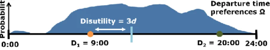
In the Hotelling choice model, we represent the attributes of both itineraries on a horizontal line, as shown in Figure 3. This is a natural representation of attributes like departure time, which are spread over the course of the day, and for which customers have heterogeneous preferences. Let represent the departure time of each flight, and draw the line such that 0:00 is on the left end of the line and 24:00 is on the right end.
Fig. 3: A Hotelling Line for Two Horizontally Differentiated Flights
We assume that customers have random departure time preferences that are spread across the day according to some distribution . It makes sense that the preferences would vary from customer to customer; perhaps some customers prefer an early flight to make a morning meeting, while others prefer a later flight to return home after a vacation. At the same prices, there is no single departure time that is preferable to another for all customers. We call attributes like departure time horizontally differentiated attributes, since customers’ preferences are heterogeneously distributed across the horizontal line. For most customers, there will not be a scheduled flight that departs at exactly their preferred departure time . We assume that customers incur a value-of-time disutility d for each hour they move away from their preferred departure time in either direction. For instance, suppose that for a particular customer, = 12pm, = 9am, and = 8pm. This customer would face disutility 3d for selecting Flight 1 and 8d for selecting Flight 2. By adding together this disutility and the price of the flight, we can compute the
perceived price of each flight: .
Customers in our model also have a maximum out-of-pocket WTP budget , which is distributed according to some distribution . could be different for different types of customers; for instance, leisure customers versus those traveling for business. If the price of an itinerary , we say the itinerary is affordable for that customer. Amongst affordable itineraries, the customer deterministically selects the itinerary with the lowest perceived price. Note that if the customer can only afford one itinerary, he or she will select that itinerary with probability 1. If a customer can afford neither itinerary, he or she will no-go and purchase nothing.
The first term in this expression represents the probability that a customer will be able to afford only Flight 1, in which case she will purchase it with probability 1. If , this term equals zero. The second term represents the probability that the customer can afford both flights, and that she will select Flight 1 because it has a lower perceived price. The probability in the expression above will depend on the
distribution of departure preferences . Specifically, it depends on the location of each customer’s relative to an indifference point :
If a customer has a departure time preference , he or she will be indifferent between selecting Flight 1 and Flight 2 at given fares and . Note that if the flights are priced identically ( = ), the indifference point will be halfway between the departure times of the two flights. Otherwise, is a function of the difference in fares between the two flights, as well as the time value-of-time disutility d.
If a customer has a departure time preference to the left of , he or she will prefer Flight 1 at fares and . If their departure time preference is to the right of , he or she will prefer Flight 2 at those fares. Note that depending on the position of and , the customer may not always select the flight with the departure time closest to her departure time preference.
This gives us enough information to compute and , as well as the probability that the customer can afford neither itinerary.
These choice probabilities can be substituted into our simultaneous dynamic pricing equation below:
The computation of these probabilities requires that airlines have estimates of three parameters: the distributions of WTP , the distributions of departure time preferences , and the value-of-time disutility d. If these distributions vary by passenger type (i.e. leisure and business), and customers can be segmented by type, then a separate set of distribution parameters would need to be estimated for each passenger type.
A simultaneous dynamic pricing engine for two flights
horizontally differentiated attribute (departure time). This method extends the
probabilistic fare-based dynamic adjustment (PFDynA) method introduced in Wittman and Belobaba (2017).
In the new simultaneous dynamic pricing engine presented in this paper, leisure
passengers are eligible for discounts from the original RM fare, and business passengers are eligible for increments. To compute the adjusted prices, the pair of prices is computed as above. We assume airlines have knowledge of the underlying departure time preference distribution and value-of-time disutility d. There are several models that exist for time-of-day departure preference, such as the Boeing Decision Window Model (Boeing, 1996). There is also a robust literature in values-of-time for transportation (e.g. Garrow et al., 2007; Mumbower et al., 2014; Seelhorst and Liu, 2015).
For WTP, we follow Wittman and Belobaba (2017) and assume that WTP in each market follows a Normal distribution for each passenger type. To parameterize these
distributions, we use a concept called an “input Q-multiplier.” A Q-multiplier is a ratio of the lowest filed fare in the market that is used to set the mean of the assumed WTP distribution. If the lowest filed fare in the market is $100, and the input Q-multiplier was 1.5, the estimated Normal distribution of passenger WTP would have a mean of $100 · 1.5 = $150. Note that if we expect WTP for business passengers to be higher than leisure passengers, we should use a higher input Q-multiplier for business passengers.
To complete the specification, we assume a coefficient of variation of k = 0.3.1
Thus, the distribution of WTP in this market would be Normal with a mean of $150 and a standard deviation of 0.3 * $150 = $45. We can then compute
where is the inverse cumulative density function of the standard Normal
distribution.
In practice, a grid search algorithm was used to find the pair of fares that maximizes expected revenue. We also bound the incremented or discounted fares of the lowest-available fare class by the adjacent higher and lower fare classes in the pre-filed fare structure. This prevents fare inversions (by ensuring the incremented fare does not rise above the unadjusted fare in the next highest class) and ensures that the RM system still has some say in deciding the range of fares that are made available. Simultaneous dynamic pricing can thus be seen as a DPE heuristic that makes small dynamic adjustments to fares that would otherwise be offered by traditional airline RM.
SIMULATION RESULTS
Simultaneous dynamic pricing was implemented and tested in the MIT Passenger Origin-Destination Simulator (PODS). PODS is an airline RM simulator that has been under
continuous development since the 1990s that models the interactions between airlines, which use RM systems to make various fare products available, and customers, who make purchasing decisions amongst those fare products. The inner workings of PODS have been documented in detail by past work; e.g. Fiig et al., 2010; D’Huart and Belobaba, 2012; and Bockelie and Belobaba, 2017.
PODS randomly generates a number of passengers for each simulation run. Each passenger is created with a customer type: either leisure or business, as well as other attributes including a maximum WTP for air travel, a preferred window of departure times; and disutilities for various fare restrictions. Business passengers are more likely to arrive later in the booking process, have a higher maximum WTP, and have higher disutilities for onerous fare restrictions than leisure passengers. PODS passengers may choose to buy up to a more-expensive, less-restricted class to avoid the restrictions from a less-expensive class, and will choose to no-go if no classes are available or affordable. Dynamic pricing was tested in several PODS networks. Network A1TWO is a network that mimics the example given earlier. It contains one market and one airline, which operates two non-stop flights in that market. The flights depart at 9am and 8pm. In the context of PODS, the 9am (morning) flight is seen as the more-attractive flight, and the 8pm (evening) flight is seen as the less-attractive flight. Network A2FOUR is an
extension of A1TWO with one market and two airlines, each of which operate a 9am and an 8pm departure. This allows us to test the performance of dynamic pricing in a
competitive environment.
In these simple networks, the airlines control availability using the leg-based EMSRb heuristic (Belobaba, 1992) and standard pick-up forecasting. A deterministic linear program (e.g. Smith and Penn, 1988) was used to calculate the bid prices for each flight leg for use in the dynamic price adjustment calculation. The so-called “EMSRc” critical value (Bratu, 1998), which is the expected marginal seat revenue of the last available seat on the aircraft, could also be used as a bid price when computing dynamic price
adjustments.
Class Fare Adv. Purch. R1 R2 R3
1 $500 N/A N N N 2 $400 3 days N N Y 3 $300 7 days N Y Y 4 $200 10 days Y N Y 5 $150 14 days Y Y N 6 $100 21 days Y Y Y Table 1: Fare structure used in Network A1TWO and A2FOUR
The airline uses a six-class restricted fare structure, which is shown in Table 1. R1, R2, and R3 represent fare restrictions, such as a Saturday night minimum stay, that are
onerous to customers. R1 is the most onerous restriction, and R3 is the least onerous. The network was calibrated in low demand (78 per cent average load factor), medium demand (83 per cent ALF), and high demand (87 per cent ALF) scenarios.
passengers. As described above, leisure passengers will only be eligible for discounts from the RM fare under dynamic pricing, and business passengers will only be eligible for increments. We also assume airlines have knowledge of the underlying departure time preference distribution used by PODS.
The value-of-time disutility d is also known to the airline, and is set to $40 per hour for business passengers and $20 per hour for leisure passengers. This 2:1 ratio of business value-of-time to leisure value-of-time is similar to that used for internal use by the U.S. Department of Transportation (U.S. Department of Transportation, 2016). In a sensitivity analysis, different input ratios between business and leisure values of time yielded similar revenues; these results are omitted here for brevity.
To specify estimates of WTP, the airlines use the Q-multiplier parameters described above. Recall that input Q-multipliers represent the airline’s estimate of WTP for each passenger type in the market, and are used to construct the distribution of WTP used by the DPE. For these tests, the airlines use an input Q-multiplier of 2.0 for business passengers and 1.5 for leisure passengers, along with a coefficient of variation of 0.3. Note that each airline does not know the exact departure time preference or actual maximum WTP for any specific customer.
Tests of dynamic pricing in a single airline network
First, we test a DPE that applies dynamic price adjustments to each flight individually, without directly incorporating the possibility of substitution. With flight-by-flight dynamic pricing, business passengers are eligible for increments and leisure passengers are eligible for discounts, as described in the previous section, and the passenger choice function for each flight does not include the prices or characteristics of other itineraries. Despite the fact that it does not explicitly consider substitution of passengers between different itineraries, flight-by-flight dynamic pricing has shown good performance in past tests, even in complex networks with many itineraries (Wittman and Belobaba, 2017). Figure 4 shows the results of using flight-by-flight dynamic pricing in the single-carrier Network A1TWO. In this network, flight-by-flight dynamic pricing increases airline revenues between 4.8 per cent over the base case in the low-demand environment and 6.5 per cent over the base case in the high-demand environment.
Fig. 4: Revenues when AL1 Uses Flight-by-Flight Dynamic Pricing (Single-Airline Network A1TWO)
Flight-by-flight dynamic pricing leads to revenue gains through several mechanisms. First, by giving discounts to selected leisure passengers, particularly those booking in higher fare classes, the airline can stimulate additional demand that otherwise would have chosen to no-go. This can increase the airline’s load factors. Also, by incrementing fares for certain business passengers, particularly those booking in lower fare classes, the airline can increase yields as well. Incrementing can also encourage some business passengers to buy-up to higher fare classes, since higher classes will become relatively more attractive when the prices of lower, heavily-restricted classes are increased. This buy-up behavior also improves the airline’s fare class mix.
Fig. 5: AL1 Load Factors (Left Panel) and Passenger Yield ($ per RPM; Right Panel) when AL1 Uses Flight-by-Flight Dynamic Pricing (Single-Airline Network A1TWO)
As Figure 5 shows, flight-by-flight dynamic pricing increases both load factors and yields in the low demand and medium demand scenarios. For instance, in medium demand, the airline’s average load factor increases from 83.0% to 84.3%, and its passenger yield increases by 4 per cent. In the high-demand scenario, load factors decline slightly as business increments and a reduction in availability in lower fare classes causes some passengers to no-go, but yields increase by 7 per cent as a result of business passenger increments and improvements in fare class mix. We will see some similar patterns in the performance of the simultaneous DPE below.
Simultaneous dynamic pricing
Figure 6 shows the results of using the simultaneous DPE described earlier, which directly models the choice of passengers between multiple flights. As the figure shows, the total revenue gains of simultaneous dynamic pricing are in the range of 5.4 to 7.4 per cent over the base case of traditional airline RM. Compared to flight-by-flight dynamic pricing, the simultaneous pricing model improves revenue performance from 0.6 to 0.9 per cent across all three demand scenarios.
Fig. 6: Revenues when AL1 Uses Flight-by-Flight Dynamic Pricing or Simultaneous Dynamic Pricing of Both Itineraries (Single-Airline Network A1TWO)
The total revenue results from Figure 6 are among the higher end of the revenue gains for dynamic pricing presented in past work (e.g. Zhang and Lu, 2013; Fiig et al., 2016; Wittman and Belobaba, 2017). However, it should be noted that the airline using simultaneous dynamic pricing is assumed to have a great deal of information about the passengers: the actual departure time preference distribution and value-of-time disutility, as well as a good estimate of leisure and business WTP and perfect passenger type identification accuracy.
When the airline uses simultaneous dynamic pricing, it sees increases in both load factor and passenger yield, as was the case with flight-by-flight dynamic pricing, as shown in Figure 7. As shown in Figure 8, the yield increases come from the increments provided to
business passengers, and from discounts that stimulate new leisure passenger bookings in higher fare classes. As a result, the more-attractive morning flight and the less-attractive evening flight both show increases in average revenue of 4.2 per cent and 9.2 per cent, respectively, over the base. Also, as Figure 7 shows, the increases in both yield and load factor from simultaneous dynamic pricing persist in all demand scenarios.
Fig. 7: Average Load Factor (Left Panel) and Passenger Yield ($ per RPM; Right Panel) with Simultaneous Dynamic Pricing
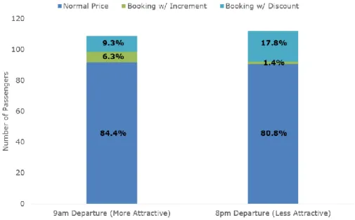
Fig. 8: Passengers on Each Flight Booking with and without Dynamic Price Adjustments with Simultaneous Dynamic Pricing
These increases in yield and load factor are possible even though most passengers book with neither an increment nor a discount. On the more-attractive morning flight, 6.3 per cent of passengers book with an increment, and 9.3 per cent book with a discount when simultaneous dynamic pricing is used, as shown in Figure 8. On the less-attractive
evening flight, just 1.4 per cent of passengers book with an increment, and 17.8 per cent book with a discount.
The targeted discounts on the evening flight shift demand from the morning flight to the evening flight, as shown in Figure 9. In the base case, the more-attractive morning flight had a higher load factor of 87.4 per cent, compared to just 78.7 per cent for the less-attractive evening flight. By discounting the evening flight for certain customers through simultaneous dynamic pricing, the load factor of the less-attractive flight increases to 86.2 per cent. Meanwhile, the load factor of the morning flight reduces to 83.7 per cent.
Fig. 9: Average Load Factors by Flight with Simultaneous Dynamic Pricing
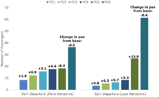
Simultaneous dynamic pricing also improves the fare class mix on both flights. Figure 10 shows that both flights see fewer bookings in the least-expensive fare class (FC) 6 when simultaneous dynamic pricing is used. This makes sense for the morning flight, since price-sensitive demand is shifted to the evening flight and fare increments encourage business passengers to buy up to higher classes on the morning flight. It is surprising to see that the fare class mix also improves on the evening flight, on which 17.8 per cent of customers booked with discounts and only 1.4 per cent booked with increments.
The rationale behind this unexpected result is a concept we refer to as “forecast spiral-up” (Wittman and Belobaba, 2017). With simultaneous dynamic pricing, discounts are
provided to leisure customers booking in relatively higher fare classes. This causes more bookings to be recorded in these higher classes. Then, the RM forecaster begins to account for the additional bookings it is seeing in higher classes by increasing demand forecasts for those classes and lowering demand forecasts for less-expensive classes.
Fig. 10: Fare Class Mix by Flight when AL1 Uses Simultaneous Dynamic Pricing
As shown in Figure 11, the RM system’s demand forecasts for fare classes 5 and 6 decrease when the airline uses simultaneous dynamic pricing, and forecasts increase for higher fare classes 1 through 4. As a result, the RM optimizer begins to protect more seats for higher classes, saving fewer seats for the lowest fare class (FC6).
Fig. 11: Initial Demand Forecasts by Fare Class when AL1 Uses Simultaneous Dynamic Pricing
Due to forecast spiral-up, we see higher bid prices and FC6 closed more often when the airline is using simultaneous dynamic pricing. We also see fewer early bookings (due to reduced availability in the least-expensive fare class relative to the base) and an increase in later bookings (due to discounts being provided to leisure customers in higher fare classes) when simultaneous dynamic pricing is used. Both of these effects combine to increase yields and load factors, leading to revenue increases from the DPE.
Adding a competitor
Finally, a competitor is added to the network which also offers an identical morning flight at 9am and an evening flight at 8pm. The competitor airline also uses EMSRb with standard pick-up forecasting, and the demand in the new network baseline is recalibrated to an average load factor of 83.5 per cent for both airlines. We will investigate two scenarios: Airline 1 (AL1) only using simultaneous dynamic pricing, and both airlines using simultaneous dynamic pricing.
Fig. 12: Airline Revenues when One or Both Airlines Use Simultaneous Dynamic Pricing
As shown in Figure 12, simultaneous dynamic pricing is revenue positive when practiced by one or both airlines. If one airline practices simultaneous dynamic pricing in this network, it sees a revenue gain of 7 per cent, while its competitor sees no revenue change (the 0.2 per cent increase is not statistically significant). If both airlines practice
simultaneous dynamic pricing, they both see revenue gains between 6 and 6.5 per cent, which is similar to the gains shown in the single-airline case in the medium-demand scenario.
When there are multiple airlines in the network, the use of simultaneous dynamic pricing by only one airline can lead to passengers shifting between carriers relative to the base. The net result of this behavior, as shown in Figure 13, is an increase in load factor for both AL1 and AL2 even when only AL1 uses simultaneous dynamic pricing.
Fig. 13: Airline Load Factors (Left Panel) and Yields ($ per RPM; Right Panel) when One or Both Airlines Use Simultaneous Dynamic Pricing
For AL1, load factors increase due to the discounts it provides to leisure passengers, although it may lose some business passengers to AL2 as a result of incrementing. AL2 is able to increase its load factor relative to the base by recapturing some of AL1’s business passengers. AL2 will also tend to have better availability in the least-expensive FC6 than AL1, which closes down FC6 more often as a result of forecast spiral-up. This means AL2 will gain more bookings in the lowest fare class, lowering its yield relative to the base. However, AL2’s increase in load factor helps compensate for its reduction in yield, leading to no significant overall change in revenue from the base. When both airlines use simultaneous dynamic pricing, they both see higher revenues, yields and load factors, as in the single-airline case.
Conclusions of simulation results
In this section, we tested our simultaneous dynamic pricing engine and compared it to previous flight-by-flight dynamic pricing approaches. We found that dynamically pricing both flights simultaneously reinforces the desirable shift in demand that it was designed to produce: namely, price-sensitive customers shift from the more-attractive 9am departure to the less-attractive 8pm departure.
However, this shift in demand leads to relatively marginal (although positive) changes in revenue over flight-by-flight dynamic pricing when each flight was priced separately. Figure 14 shows that flight-by-flight dynamic pricing also naturally leads to lower load factors on the morning flight (through incrementing) and higher load factors on the evening flight (through discounting), even without directly considering the
Fig. 14: Load Factors by Flight when AL1 Uses Flight-by-Flight Dynamic Pricing or Simultaneous Dynamic Pricing of Both Itineraries (Single-Airline Network A1TWO)
While it is encouraging that simultaneously pricing both flights together leads to higher revenues than pricing each flight separately, recall that the airline using the simultaneous dynamic pricing heuristic was assumed to know a significant amount of additional information: the actual underlying departure time preference distribution, as well as the value of time disutilities for each passenger type. Even under this very optimistic assumption, the additional revenue gain over dynamic pricing of each flight independently was less than one per cent. This is good news for dynamic pricing practitioners, as it suggests that simple models for customer choice could capture the majority of revenue gains from dynamic pricing.
CONCLUSIONS AND EXTENSIONS
In this paper, we introduced and tested a new methodology for a dynamic pricing engine (DPE) to simultaneously price two flights with different departure times. In contrast to other approaches, which use multinomial logit choice models, we used a locational choice model to frame customers’ purchasing decisions based on their willingness to pay and departure time preferences. We then described a simultaneous dynamic pricing method which applied increments or decrements to the lowest-available fares that are output by an airline’s RM system.
Through simulations in the Passenger Origin-Destination Simulator (PODS), we found that simultaneous dynamic pricing led to revenue gains of between 5 and 7 per cent over the base case in a simple network with one airline, one market, and two non-stop flights. This heuristic performance was at the upper range of dynamic pricing heuristics reported in the literature, but also assumed that airlines could accurately segment booking requests into leisure and business categories, and possessed good information about the departure time preferences and value-of-time disutilities of their customers.
However, simultaneous dynamic pricing produced gains of less than one per cent over a version of dynamic pricing that priced each flight independently. In other words, a simple customer choice model was able to capture most of the revenue gains of dynamic pricing, and additional complexity added only marginal benefits. Given the challenges of
estimating and implementing a simultaneous DPE in practice, practitioners may be content to rely on flight-by-flight dynamic pricing, at least for early DPE adaptations. If airlines do begin simultaneously pricing itineraries with DPEs, there are several directions in which this work could be extended to make the model more relevant to different choice environment. For instance, additional itinerary quality attributes could be added to the choice model, and the presence of competitors could also be introduced into the customer choice function. It would also be possible to increase the number of
customer segments that the airline can identify. A more complex choice model that incorporates additional attributes could potentially further improve the performance of simultaneous dynamic pricing.
Finally, the simultaneous choice model within the DPE could be extended to three or more flights. This is a doable yet cumbersome mathematical exercise, because it requires that the algorithm considers each combination of possible choice sets. Given the marginal gains of two-flight simultaneous dynamic pricing over the flight-by-flight approach, the addition of further flights to the choice model would likely show decreasing returns to scale.
ACKNOWLEDGMENTS
Michael Wittman would like to thank Craig Hopperstad for excellent development assistance with PODS; members of the MIT PODS Consortium for funding and helpful suggestions; participants of the 2017 AGIFORS RM Study Group Meeting; and Jan Vilhelmsen, Robin Adelving, and Jean-Michel Sauvage for their hospitality during the author’s research visit at Amadeus in August 2016.
REFERENCES
Akçay, Y., H.P. Natarajan, and S.H. Xu. 2010. Joint Dynamic Pricing of Multiple Perishable Products Under Consumer Choice. Management Science 56(8): 1345-1361.
Aydin, G. and J.K. Ryan. 2000. Product line selection and pricing under the multinomial logit model. Proceedings of the 2000 MSOM Conference, Ann Arbor, MI. 1-49.
Belobaba, P.P. 1992. Optimal vs. heuristic methods for nested seat allocation. Presentation to AGIFORS reservations control study group meeting, Brussels, Belgium.
Belobaba, P.P. 2016. Optimization models in RM systems: Optimality versus revenue gains. Journal of Revenue and Pricing Management 15(3): 229-235.
Bockelie, A. and P.P. Belobaba. 2017. Incorporating Ancillary Services in Airline Passenger Choice Models. Journal of Revenue and Pricing Management. Forthcoming.
Boeing. 1996. The Decision Window Path Preference Model: Summary Discussion. Marketing and Business Strategy, Boeing Commercial Airplanes.
Bratu, S. 1998. Network Value Concept in Airline Revenue Management. Unpublished Master’s Thesis, Massachusetts Institute of Technology, Cambridge, MA.
Burger, B. and M. Fuchs. 2005. Dynamic pricing — A future airline business model. Journal of Revenue and Pricing Management4(1): 39-53.
Chen, S., G. Gallego, M.Z.F. Li, and B. Lin. 2010. Optimal seat allocation for two-flight problems with a flexible demand segment. European Journal of Operations Research 201: 897-908.
D’Huart, O. and P. Belobaba. 2012. A model of competitive airline revenue management interactions. Journal of Revenue and Pricing Management 11(1): 109-124.
Dong, L., P. Kouvelis, and Z. Tian. 2009. Dynamic Pricing and Inventory Control of Substitute Products. Manufacturing and Service Operations Management 11(2): 317-339.
Fiig, T., K. Isler, C. Hopperstad, and P.P. Belobaba. 2010. Optimization of Mixed Fare
Structures: Theory and Applications. Journal of Revenue and Pricing Management 9(1-2): 152-170.
Fiig, T., U. Cholak, M. Gauchet, and B. Cany. 2015. What is the role of distribution in revenue management? – Past and future. Journal of Revenue and Pricing Management 14(2): 127-133. Fiig, T., O. Goyons, R. Adelving, and B. Smith. 2016. Dynamic pricing – The next revolution in RM? Journal of Revenue and Pricing Management. Published online in Articles in Advance. Gallego, G. and R. Wang. 2014. Multiproduct Price Optimization and Competition Under the Nested Logit Model with Product-Differentiated Price Sensitivities. Operations Research 62(2): 450-461.
Garrow, L., S.P. Jones, and R.A. Parker. 2007. How much airline customers are willing to pay: An analysis of price sensitivity in online distribution channels. Journal of Revenue and Pricing Management 5(4): 271-290.
Gaur, V. and D. Honhon. 2006. Assortment Planning and Inventory Decisions Under a Locational Choice Model. Management Science 52(10): 1528-1543.
Mumbower, S., L.A. Garrow, and M.J. Higgins. 2014. Estimating flight-level price elasticities using online airline data: A first step toward integrating pricing, demand, and revenue
optimization. Transportation Research Part A: Policy and Practice 66: 196-212.
Ratliff, R. 2017. Industry-standard Specifications for Air Dynamic Pricing Engines: Progress Update. Proceedings of the 2017 AGIFORS Revenue Management Study Group Meeting, San Francisco, CA
Seelhorst, M. and Y. Liu. 2015. Latent air travel preferences: Understanding the role of frequent flyer programs on itinerary choice. Transportation Research Part A: Policy and Practice 80: 49-61.
Smith, B.C. and C.W. Penn. 1988. Analysis of alternative origin-destination control strategies. AGIFORS Symposium Proceedings 28: New Seabury, MA.
Suh, M. and G. Aydin. 2011. Dynamic pricing of substitutable products with limited inventories under logit demand. IIE Transactions 43: 323-331.
U.S. Department of Transportation. 2016. The Value of Travel Time Savings: Departmental Guidance for Conducting Economic Evaluations Revision 2 (2016 Update). 27 September 2016. Westermann, D. 2013. The potential impact of IATAs New Distribution Capability (NDC) on revenue management and pricing. Journal of Revenue and Pricing Management 12(6): 565-568. Wittman, M.D. and P.P. Belobaba. 2017. Customized dynamic pricing of airline fare products. Journal of Revenue and Pricing Management. Available online 9 October 2017.
Zhang, D. and W. L. Cooper. 2009. Pricing substitutable flights in airline revenue management. European Journal of Operations Research 197: 848-861.
Zhang, D. and Z. Lu. 2013. Assessing the Value of Dynamic Pricing in Network Revenue Management. INFORMS Journal on Computing 25(1): 102-115.