Does Competition Reduce Costs? Assessing the Impact of Regulatory Restructuring on U.S. Electric Generation
Efficiency
by
04-018 November 2004
Nancy L. Rose, Kira Markiewicz, and Catherine Wolfram
Does Competition Reduce Costs?
Assessing the Impact of Regulatory Restructuring
on U.S. Electric Generation Efficiency
Kira Markiewicz
UC Berkeley, Haas School of Business
Nancy L. Rose
MIT and NBER
Catherine Wolfram
UC Berkeley and NBER
∗November 2004
∗markiewi@haas.berkeley.edu, nrose@mit.edu, wolfram@haas.berkeley.edu. Rose acknowledges support
from the MIT Center for Energy and Environmental Policy Research and the Hoover Institution. We thank participants at the NBER Productivity Program Meeting, the NBER IO Summer Institute Meeting, the University of California Energy Institute POWER conference, and the MIT Center for Energy and
Environmental Policy Research conference, as well as seminar participants at Harvard, MIT, UC Berkeley, UC Davis and Yale for their suggestions. We are particularly grateful for the detailed comments on earlier drafts provided by Al Klevorick, Mark Roberts, Charles Rossman and Johannes Van Biesebroeck. We also thank Tom Wilkening for assistance in coding restructuring policy characteristics across states.
Does Competition Reduce Costs?
Assessing the Impact of Regulatory Restructuring
on U.S. Electric Generation Efficiency
Kira Markiewicz
Nancy L. Rose
Catherine Wolfram
Abstract
Although the allocative efficiency benefits of competition are a tenet of microeconomic theory, the relation between competition and technical efficiency is less well understood. Neoclassical models of profit-maximization subsume static cost-minimizing behavior regardless of market competitiveness, but agency models of managerial behavior suggest possible scope for
competition to influence cost-reducing effort choices. This paper explores the empirical effects of competition on technical efficiency in the context of electricity industry restructuring.
Restructuring programs adopted by many U.S. states made utilities residual claimants to cost savings and increased their exposure to competitive markets. We estimate the impact of these changes on annual generating plant-level input demand for non-fuel operating expenses, the number of employees and fuel use. We find that municipally-owned plants, whose owners were for the most part unaffected by restructuring, experienced the smallest efficiency gains over the past decade. Investor-owned utility plants in states that restructured their wholesale electricity markets had the largest reductions in nonfuel operating expenses and employment, while investor-owned plants in nonrestructuring states fell between these extremes. The analysis also highlights the substantive importance of treating the simultaneity of input and output decisions, which we do through an instrumental variables approach.
JEL Codes:
L11, L43, L51, L94, D24
Keywords:
Efficiency, Production, Competition, Electricity restructuring, Electric
Generation, Regulation
Economists have long argued that competition generates important efficiency benefits for an economy. These generally focus on allocative efficiency; the implications of competition for technical efficiency are less clear. Neoclassical models of profit-maximization subsume static cost-minimizing behavior by all firms, regardless of market competitiveness.1 Agency models,
however, in recognizing the interplay of asymmetric information with the separation of management and control, suggest possible deviations from cost-minimization by effort-averse managers. These models may imply a role for competition in constraining managerial behavior, by rewarding efficiency gains and confronting less-efficient firms with the choice of cost reduction to the level of their lower-cost counterparts or exit; see Nickell (1996) for a brief discussion of some of these theoretical arguments. Their actual relevance is ultimately an empirical question.
This paper assesses the effect of competition on technical efficiency using data on the U.S. electric generation sector. The past decade has witnessed a dramatic transformation of this industry. Until the mid-1990s, over ninety percent of the electricity in the US was sold by vertically-integrated investor-owned utilities (IOUs), most operating as regulated monopolists within their service areas. Today, non-utility generators own roughly a quarter of generation capacity nationwide, and IOUs in many states own only a small fraction of total generating capacity and operate in a partially deregulated structure that relies heavily on market-based incentives or competition. While studies of state-level electricity restructuring suggest politicians may have been motivated in large part by rent-seeking (e.g., White, 1996, and Joskow, 1997), many proponents of restructuring argued that exposing utilities to competitive, market-based outcomes would yield efficiency gains that could ultimately reduce electricity costs and retail prices. Research on other industries suggests productivity gains associated with deregulation (e.g., Olley and Pakes, 1996, on telecommunications and Ng and Seabright, 2001, on airlines) and with increased competitive pressure caused by factors other than regulatory change (e.g., Galdón-Sánchez and Schmitz, 2002, on iron ore mines).2
1 The implication of competition for dynamic efficiency through innovation is the subject of an extensive
theoretical and empirical literature in economics, dating at least from Schumpeter’s 1943 classic
Capitalism, Socialism, and Democracy.
2 Some hint of this possibility in electricity is provided by Primeaux (1977), who compared a sample of
municipally owned firms facing competition to a matched sample of municipally owned firms in monopoly situations and found a significant decrease in costs per kWh for firms facing competition.
The considerable body of academic work on electricity restructuring within the U.S. and abroad has thus far focused on assessing the performance of competitive wholesale markets, with particular attention to the exercise of market power (see for example Borenstein, Bushnell and Wolak, 2002 and Joskow and Kahn, 2002). While many of the costs of electricity restructuring have been intensively studied, relatively little effort has been devoted to quantifying any ex post operating efficiency gains of restructuring, although a few studies (e.g., Knittel, 2002) have analyzed efficiency effects of various incentive regulations in this sector.3 This study provides
the first substantial analysis of early generation efficiency gains of electricity restructuring. As such, it contributes to the broad economic debate on the role of competition in the economy and is of direct policy relevance to states contemplating the future of their electricity restructuring programs.
The results of this work indicate that plant operators most affected by restructuring reduced labor and nonfuel expenses, holding output constant, by roughly 5% or more relative to other investor-owned utility (IOU) plants, and by 15-20% relative to government- and cooperatively-investor-owned plants, which were largely unaffected by restructuring incentives. These may be interpreted as the medium-run efficiency gains that Joskow (1997, p. 214) posits “may be associated with improving the operating performance of the existing stock of generating facilities and increasing the productivity of labor operating these facilities.” Our work also highlights the importance of treating the simultaneity of input and output choice. Failing to recognize that shocks to input productivity may induce firms to adjust targeted output leads to overstatement of estimated efficiency effects, in some cases by a factor of two or more. While endogeneity concerns have been long recognized in the productivity literature, ours is one of the first studies of electric generation to compensate for this. Finally, we explore the sensitivity of the estimated efficiency impact to the choice of control group to which restructured plants are compared, and discuss the issues involved in determining the appropriate counterfactual.
3 One exception is Hiebert (2002), who uses stochastic frontier production functions to estimate generation
plant efficiency over 1988-1997. One set of independent variables he includes is indicators for regulatory orders or legislative enactment of restructuring reforms in 1996 and in 1997. While he finds significant reductions in mean inefficiency associated with restructuring laws in 1996 for coal plants, he finds no effects for gas plants, nor for either fuel type in 1997. Our work uses a longer time period, richer characterization of the restructuring environment and dating of reforms consistent with the U.S. Energy Information Administration, and an alternative technology specification that allows for more complex productivity shocks and treats possible input endogeneity biases. Joskow (1997) describes the significant labor force reductions that accompanied restructuring in the UK, as the industry moved from state-owned monopoly to a privatized, competitive generation market, although these mix restructuring and
The remainder of the paper is organized as follows: Section 1 describes existing evidence on the competitive effects of efficiency, and discusses how restructuring might alter electric generation efficiency. Section 2 details our empirical methodology for testing these predictions, and describes our strategy for identifying restructuring effects. The data are described in Section 3. Section 4 reports the results of the empirical analysis, and Section 5 concludes.
1. Why Might Restructuring Affect Generator Efficiency?
Exit by less-efficient firms is a well-understood efficiency benefit of competition: as output shifts from (innately) higher-cost firms to lower-cost competitors the total production cost for a given output level decline. Olley and Pakes (1996) provide empirical evidence of this phenomenon in their plant-level analysis of the magnitude and source of productivity gains in the U.S.
telecommunications equipment industry over 1974-1987. They find substantial increases in productivity associated with the increased competition that followed the 1984 divestiture and deregulation in this sector, and identify the primary source of these gains as the re-allocation of output from less productive to more productive plants across firms. In a similar vein, Syverson (2004) finds that more competitive local markets in the concrete industry are associated with higher mean, less dispersion, and higher lower-bounds in plant productivity, effects he attributes to the exit of less-efficient plants in more competitive environments.
The existing evidence on whether competition also leads to cost reductions through technical efficiency gains by continuing producers and plants is relatively sparse. Nickell (1996) uses a panel of 670 U.K. manufacturing firms to estimate production functions that include controls for the competitive environments in which firms operate. He finds some evidence of reduced productivity levels associated with market power and strong support for higher productivity growth rates in more competitive environments. Concerns about the ability of cross-industry analysis to control adequately for unobservable heterogeneity across sectors may make sector-specific evidence tighter and more convincing.4 A notable example is the Galdón-Sánchez and Schmitz (2002) study of labor productivity gains at iron ore mines that faced increased
competitive pressure following the collapse of world steel production in the early 1980s. They find unprecedented rates of labor productivity gains associated with this increase in competitive
4 A number of studies have analyzed efficiency gains following regulatory reform in various industries;
see, for example, Bailey’s (1986) overview and Park et al. (1998) on airlines. Unfortunately, in many cases it is difficult to disentangle direct regulatory effects on efficiency (e.g., operating restrictions imposed on trucking firms or airlines by regulators in those sectors) from the indirect effects of reduced
competition.
pressure, “driven by continuing mines, producing the same products and using the same technology as they had before the 1980s” (Galdón-Sánchez and Schmitz, 2002, p. 1233).5
Several features of the electric generation sector make it an attractive subject for testing potential competitive effects on technical efficiency.6 First, generation technology is reasonably stable and well-understood and data on production inputs and outputs at the plant-level are readily available to researchers. This has made electric generation a common application for new production and cost function estimation techniques, dating at least to Nerlove (1963). Second, policy shifts over a relatively short period have resulted in a dramatic transformation of the market for electric power. Through the early 1990s, the U.S. electricity industry was dominated by vertically integrated investor-owned utilities (IOUs). Most operated as regulated monopolists over
generation, transmission, and distribution of electricity within their localized geographic market, though there was some wholesale power traded among utilities or purchased from a small but growing number of non-utility generators. Prices generally were determined by state regulators based on accounting costs of service at the firm level. By 1998, every jurisdiction (50 states and the District of Columbia) had initiated formal hearings to consider restructuring their electricity sector, and by 2000, almost half had approved legislation introducing some form of competition including retail access.7 This provides both time series and geographic variation in competitive environments. Third, static and dynamic efficiency claims bolstered much of the policy reform; measuring these benefits is a vital prerequisite to assessing the wisdom of these policies.
It has long been argued that traditional cost-of-service regulation does relatively well in limiting rents but less well in providing incentives for cost-minimizing production; see Laffont and Tirole (1993). Under pure cost-of-service regulation, regulator-approved costs of the utilities are passed directly through to customers, and reductions in the cost of service yield at most short-term profits until rates are revised to reflect the new lower costs at the next rate case.8 Given asymmetric information between regulators and firms, inefficient behavior by managers that raises operations costs above minimum cost levels generally would be reflected in increased rates
5 Ng and Seabright (2001) estimate cost functions for a panel of U.S. and European airlines over
1982-1995, and conclude that potential gains from further privatization and increased competition among European carriers are substantial, though they point out that the best-measured component of these gains relates to ownership rather than market structure differences.
6 Understanding possible reallocation of output across plants is hampered by the exit of plants from most
available databases when they are sold to non-utility owners.
7 In the aftermath of California’s electricity crisis in 2000-2001, restructuring has become less popular and
many states have delayed or suspended restructuring activity, including six that had previously approved retail access legislation. See US Energy Information Administration (EIA), 2003.
and passed through to customers. Joskow (1974) and Hendricks (1975) demonstrate that frictions in cost-of-service regulation, particularly those arising from regulatory lag (time between price-resetting hearings), may provide some incentives at the margin for cost-reducing effort. Their impact generally is limited, however, apart from periods of rapid nominal cost inflation (see Joskow, 1974).
This system led economists to argue that replacing cost-of-service regulation with
higher-powered regulatory incentive schemes or increased competition could enhance efficiency.9 Over
the 1980s and early 1990s, many state utility commissions accordingly adopted some form of incentive regulation. The limited empirical evidence available on these reforms, which modify price setting within the regulated monopoly structure, suggests mixed results. Knittel (2002) studies a variety of incentive regulations in use through 1996, and finds that those targeted at plant performance or fuel cost were associated with gains in plant-level generation efficiency.10 More general reforms, such as price caps, rate freezes, and revenue-decoupling programs, typically were associated with insignificant or negative efficiency estimates, all else equal.
Restructuring, in contrast to incentive regulations, fundamentally changed the way plant owners earn revenue. At the wholesale level, plants sell either through newly created spot markets or through long-term contracts that are presumably based on expected spot prices. In the spot markets, plant owners submit bids indicating the prices at which they are willing to supply power from their plants. Dispatch order is set by the bids, and, in most markets, the bid of the marginal plant is paid to all plants that are dispatched. High-cost plants will be forced down in the dispatch order, reducing likely revenue. Plant operators that reduce costs move higher in the dispatch order, increasing dispatch probability, and increase the profit margin between own costs and the expected market price. Most restructuring programs also changed the way retail rates are determined and the way in which retail customers are allocated.11 Retail access programs in
8 Rates are constant between rate cases, apart from certain specific automatic adjustments (such as fuel
adjustment clauses), so changes in cost would not be reflected in rates until the next rate case.
9 See, for example, Laffont and Tirole, 1993, for a theoretical justification, or Joskow and Schmalensee,
1987, for an applied argument.
10 Knittel uses OLS and stochastic production frontier techniques to estimate Cobb-Douglas generating
plant production functions in capital, labor, and fuel for a panel of large IOU plants over 1981-1996. His results from first-differenced models, which implicitly allow for plant-level fixed efficiency effects, suggest gains on the order of 1-2% associated with these reforms. Equations that do not allow for plant fixed effects suggest much larger magnitudes.
11 States have used a variety of approaches to link retail rates under restructuring to wholesale prices in the
market. Over the short term, most states decoupled utility revenue from costs by mandating retail rate freezes, often at levels discounted from pre-restructuring prices. Some states, such as Pennsylvania, are aggressively trying to encourage entry by competitive energy suppliers, who may contract directly with retail customers.
combination with the creation of the new wholesale spot markets may increase the intensity of cost-cutting incentives, leading to even greater effort to improve efficiency.
While the most significant savings from restructuring are likely to be associated with efficient long-run investments in new capacity, there may be opportunities for modest reductions in operating costs of existing plants (see Joskow, 1997). This paper attempts to measure the extent of that possible improvement for the existing stock of electricity generating plants in the U.S. The implicit null hypothesis is that, before restructuring, operators were minimizing their costs, given the capital stock available in the industry. Under the null, there should be no change in plant-level efficiency measures associated with restructuring activity. We discuss below our method for estimating plant efficiency and identifying deviations from this hypothesis. Assessing the effects of restructuring requires specification of how generating plants would have been operated absent the policy change. Constructing this counterfactual is crucial, but difficult.
2. Empirical Model
For a single-output production process, productive efficiency can be assessed by estimating whether a plant is maximizing output given its inputs and whether it is using the best mix of inputs given their relative prices. Production functions describe the technological process of transforming inputs to outputs and ignore the costs of the inputs; a plant is efficient if it is on the production frontier. Cost minimization assumes that, given the input costs, firms choose the mix of inputs that minimizes the costs of producing a given level of output. A plant could be
producing the most output possible from a given input combination, but not minimizing costs if, for instance, labor was cheap relative to materials, yet the plant used a lot of materials relative to labor. Even if the firm were producing the maximum output possible from its workers and materials, it would not be efficient if it could produce the same level of output less expensively by substituting labor for materials. We explore the impact of restructuring on efficiency by specifying a production function and then deriving the relevant input demand equations implied by cost minimization.
We adopt the convention of representing generating plant output (Q) by the net energy the generating units produce over some period (measured by annual megawatt-hours, MWh, in our data), a choice that is discussed in further detail in the data section below. While a multitude of studies of electric plant productivity model this output as a function of current inputs, often using a Cobb-Douglas production or cost function, the characteristics of electricity production argue strongly for an alternative specification. We derive a model of production and cost minimization
that is sensitive to important institutional characteristics of electricity production that have been largely ignored in the earlier literature.
First, observed output in general will be the lesser of the output the plant is capable of producing, given its available inputs, and the output called for by the system dispatcher. Because the system dispatcher must balance total production with demand at each moment, the gap between probable (QP) and actual (QA) output for a given plant i will be a function of demand realizations, the set of
other plants available for dispatch, and plant i’s position in the dispatch order.12
Second, while fuel inputs are varied in response to real-time dispatching and operational changes, other inputs to a plant’s production are determined in advance of output realizations. Capital typically is chosen at the time of a unit’s construction (or retirement), and at the plant level is changed relatively infrequently. From the manager’s perspective, it may be considered a fixed input. Utilities hire labor and set operating and materials expenditures in advance, based on expected demand. While these can be adjusted over the medium-run, staffing decisions as well as most maintenance expenditures are not tied to short-run fluctuations in output.13 We therefore treat these as set in advance of actual production, and determining a target level of probable output, QP.
Finally, while labor, materials, and capital may be to some extent substitutable to produce
probable output, the generation process generally does not allow these inputs to substitute for fuel in the short-run. Given this description of the technology, we posit a Leontief production process for plant i in year t of the following form:
QitA = min[ g(Eit, Γ E, εitE ), QitP(Ki, Lit, Mit, Γ P, εitP)·exp(εitA))]
where QA is actual output and QP is probable output; inputs are denoted by E for energy (fuel)
input, K for capital, L for labor, and M for materials; Γ denotes parameter vectors, and ε denotes unobserved (to the econometrician) mean zero shocks. See Van Biesebroeck (2003) for the derivation of a similar production function he uses to model automobile assembly plant production.
12 Random shocks to a plant’s operations, such as unexpected equipment failures or equipment that lasts
longer than expected, will cause it to produce less or more than its probable output from a set of available inputs.
As noted above, fuel input decisions are made in real time, after the manager has observed any shocks associated with the plant’s probable output productivity, εitP, the actual operation of the
plant, εitA, and the plant’s energy-specific productivity in the current period, εitE . Probable
output, QP, is in contrast determined by input decisions made in advance of actual production. We assume that capital, measured by the nameplate generating capacity of the plant, is fixed.14
Labor and materials decisions are made in advance of production, but after the level and productivity of the plant’s capital is observed. This reflects the quasi-fixity of these inputs over time: staffing decisions and maintenance plans are designed to ensure that the plant is available when it is dispatched, based on the targeted output QP. The error term ε
itP incorporates
productivity shocks that we assume are known to the plant manager in advance of scheduling labor and materials inputs, but are not observable to the econometrician. We allow actual output to differ from probable output by a multiplicative shock exp(εitA), assumed to be observed at the
time fuel input choices are made but not known at the time probable output is determined. This shock would be, for example, negative if a generating unit were unexpectedly shut down due to a mechanical failure, or positive if the plant were run more intensively than anticipated, as might be the case if a number of plants ahead of it in the usual dispatch order were unavailable or demand realizations were unexpectedly high.
We model probable output (QP) with a Cobb-Douglas function of labor and materials and
embedding capital effects in a constant (Q0(K)) term. This yields the specification:
(PF1) QitP ≤ Q0(Ki)·(Lit)γL·(Mit)γM· exp(εitP)
In preliminary analysis, we estimated the parameters of the production function, including terms that allowed for differential productivity under restructuring. Those results suggested
productivity gains associated with restructuring. The work reported here imposes an additional constraint, based on cost-minimization, to estimate input demand functions, and isolate possible restructuring effects on each measured input. A cost-minimizing plant manager, facing wages Wit
and material prices Sit, would solve for the optimal inputs to produce probable output QitP by:
13 In fact, over a short time period, maintenance and repair expenditures will be inversely related to output
since the boiler needs to be cool and the plant offline for most major work. We deal with this potential simultaneity bias below.
14 The empirical analysis defines a new plant-epoch, i, whenever there are significant changes in capacity,
min Wi t·Li t + Si t·Mi t s.t. Qi tP ≤ Q0(Ki)·(Li t)γL·(Mi t)γM·exp(εi tP)
Li t, Mi t
yielding the following factor demand equations:
(L1) Li t = (λγL QitP)/Wi t
(M1) Mi t = (λγM QitP)/Si t
where λ is the Lagrangian on the production constraint.
We observe actual output, QitA = QitPεitA, rather than probable output, QitP. Making this
substitution and taking logs of both sides, (L1) becomes:
(L2) ln(Li t) = α0 + ln(Qi tA) – εi tA – ln(Wi t )
where α0 = ln(λγL). If there are differences across plants, over time, or across regulatory regimes
in the coefficients of the production function (γL) or in the shadow value of the probable output
constraint (λ), or if there is measurement error in labor used at the plant, this equation will hold with error. As we are particularly interested in changes in input demand associated with restructuring, we expand the subscript it to irt to include plant i in year t, and regulatory restructuring regime r, and re-write (L2) as: 15
(L2’) ln(L irt) = ln(Q irt A) – ln(W irt ) + αiL + δtL + φ r L – ε irt A + εir tL
where αiLmeasures a plant-specific component of labor demand, δtL captures year-specific
differences in labor demand, φ r L captures restructuring-specific shifts in labor demand, and εirtL
measures the remaining error in the labor input equation. α0 is now subsumed in the plant-specific
demand, αiL. Note that φ r L picks up mean residual changes in labor input for a plant in a
restructured regime relative to that plant overall and to all other plants at the same point in time. It could reflect systematic changes in the marginal productivity of labor (γL), in the shadow value
of the availability constraint (λ) or in optimization errors. 16
15 Note that many plant-level differences, such as capital stock, and many time-varying shocks, such as
technology-neutral productivity shocks, drop out of this equation through the conditioning on output choice.
16 If there were systematic differences in the relation of probable and actual output across restructuring, γ r L
may also reflect the change in mean ε irt A. Since ε irt Areflects shocks unobservable by the firm when
setting planned output, it seems plausible that these be mean zero in expectation, but their realizations could be nonzero in the restructuring sample we observe.
Similarly, equation (M1) becomes:
(M2) ln(Mirt) = ln(QrtA) – ln(Srt ) + αiM + δtM + φ r M – ε irt A + ε ir tM
which is directly analogous to (L2’).
We model the energy component of the Leontief production function, which will in general hold with equality, as:
(PF2) QirtA = g(Eirt, γE, εE)
Assuming that g(•) is monotonically increasing in E, we can simply invert it to get an expression for E in terms of Q. Note that the price of fuel does not enter into the demand for fuel except through the level of output the plant is dispatched to produce. For consistency with the other input specifications, we specify a log-log relationship:
(E1) ln(Eirt) = γQE ·ln(Qirt) + φ r E + αiE + δtE + εirtE
where as before, the plant-specific error, αiE, the year-specific error, δtE , and the
restructuring-specific term, φ r E , capture systematic changes in the efficiency with which plants convert
energy to electricity—that is, changes in plant heat rates—across plants, over time, or correlated with restructuring activity, respectively.
We confront two important endogeneity concerns in estimating the basic input demand equations, (L2’), (M2) and (E1). The first is the possibility that shocks (ε ir tL, ε ir tM, εirtE) in the input demand
equations may be correlated with output. If output decisions are made after a plant’s manager observes the plant’s efficiency, managers may increase planned output in response to positive shocks to an input’s productivity, or reduce planned output in response to negative shocks. This behavior would induce a correlation between the error in the input demand equation and observed output. Though one can control directly for plant-specific efficiency differences and for secular productivity shocks in a given year, idiosyncratic shocks remain a source of possible bias. Second, the estimates may be subject to selection bias if exit decisions are driven by unobserved productivity shocks. In this case, negative shocks could lead to plant shutdown, implying that the
errors for observations we observe will be drawn from a truncated distribution. Neither of these problems is unique to our setting, and they have been raised in many earlier papers.17
Consider first the simultaneity issue. We face a potential simultaneity problem if, for instance, a malfunctioning piece of equipment reduces the plant’s fuel efficiency, leading the utility to reduce its operation of that plant and consequently to use less fuel. There may be deviations from predetermined employment and materials budgets caused by unanticipated breakdowns that require increased use of labor and repair expenditures and result in lower output. A positive efficiency shock to an input may lead managers to run that plant more intensively over the year, increasing output as well as input use. A variety of methods have been used to address this concern.18 We choose to use an instrumental variables approach, using a measure of state-level
electricity demand as an instrument for plant output. This is likely to be highly correlated with the amount of output a plant will be called to provide, but uncorrelated, for instance, with how efficiently an individual plant’s feedwater pumps are working. This approach is likely to be particularly effective for the energy equation, given the responsiveness of energy input choices to demand fluctuations in real time, and for identifying exogenous output fluctuations at non-baseload plants, which are more strongly influenced by marginal swings in demand. It may be less powerful in identifying variation in ex ante labor and maintenance choices, depending in part on the extent to which plant managers anticipate state demand.19 We therefore explore the
sensitivity of our results to alternative instruments.
The potential selection issue is more difficult to address. The plants in our sample seem more stable than those studied in many other contexts (especially see Olley and Pakes, 1996), suggesting that the selection problem may be somewhat less severe for electric generation. However, plant exit increases in restructuring regimes, typically not because the plant is retired but because divestitures remove the plants from the reporting database. To the extent that the divestitures are mandated by the restructuring legislation, this should not create selection
problems. But without better information on what determines discretionary divestitures, we have
17 Nerlove (1963) provides an early discussion of simultaneity bias in production functions. Olley and
Pakes (1996) propose a structural approach to addressing simultaneity, which is compared to alternatives in Griliches and Mairesse (1998). Ackerberg and Caves (2003) discuss this issue and compare treatments proposed by Olley and Pakes (1996) and Levinsohn and Petrin (2003). While many papers have estimated production or cost functions for electric generating plants, from the classic analyses in Nerlove (1963) and Christensen and Greene (1976) to very recent work such as Kleit and Terrell (2001) and Knittel (2002), electricity industry studies typically have not treated either simultaneity or selection problems.
18 See the references cited in note 17, supra.
19 A further drawback to this instrument is that we measure demand only at the state, rather than plant
no direct way to assess their impact on the results. One indirect way to assess the significance of potential selection effects is to compare results for the unbalanced panel we use in most of our work to those for a panel of plants that continue to operate through the end of our sample period, for which potential selection effects are likely to be most severe. Substantial differences across those results may suggest the need to more carefully treat potential selection biases.
Identification strategy
There is substantial heterogeneity across plants, utilities and states, and the economic environment in which utilities operate has changed considerably over time. In addition,
restructuring is not randomly assigned across political jurisdictions—earlier work suggests that it is strongly correlated with higher than average electricity prices in the cross-section.20
Fortunately, we have in this sector a database rich in variation. There are thousandsof generating plants operated by hundreds of utilities subject to regulation by dozens of political jurisdictions each setting their own legal and institutional environment. Panel data on the costs and operations of these plants are available, with some recent exceptions, from well before any restructuring until the present.21 This allows us to construct benchmarks that we believe control for most of the
potentially confounding variation.
The plant-specific effects, {αiN}, measure the mean use of input N at plant i relative to other
plants in the sample. These effects may be associated with differences in plant technology type and vintage, ownership (government v. private utilities), and time-invariant state effects. The year-specific shock, {δtN}, measures the efficiency impact of sector-level shifts over time, such as
secular technology trends, macroeconomic fluctuations or energy price shocks. Restructuring effects on plant productivity correspond to a non-zero {φrN}. The heterogeneity in the timing and
outcomes of state-level restructuring activity allow the data to distinguish between temporal shocks and restructuring effects. While all states held hearings on possible restructuring, the earliest was initiated in 1993 and the latest in 1998. There is considerable variation in the
outcome of those hearings, as well, with just under half the jurisdictions (23 states and the District of Columbia) enacting restructuring legislation between 1996 and 2000.22 The remainder
20 The significant role of sunk capital costs in regulatory ratemaking means that high prices do not
necessarily imply high operating costs for generation facilities within a state, however. See Joskow (1997) for a discussion of the contributors to price variation across states.
21 Cost data are not publicly available for plants owned by exempt wholesale generators, including those
acquired from regulated utilities.
22 We collected information on state restructuring legislation from various Energy Information
considered and rejected, or considered and simply did not act on, such legislation. This variation allows us to use changes in efficiency at plants in states that did not pass restructuring legislation to identify restructuring separately from secular changes in efficiency of generation plants over time.
It is possible that plants in this control group also altered their behavior over the post-1992 period. This could be due perhaps to the introduction or intensification of incentive regulation within states that did not enact restructuring, to the expectation of potential restructuring that did not occur, or spillovers from restructuring movements in other states (e.g. if regulators updated their information about the costs necessary to run plants of a certain type, or multi-state utilities operating under differing regimes improved efficiency of all their plants, not just those in restructuring states). To the extent this occurs, our comparison will understate the magnitude of any efficiency effect of restructuring.
We therefore consider a second control group, consisting of cooperatively-owned or publicly-owned municipal and federal plants, which for convenience we will refer to as “MUNI” plants, although the group is broader than strictly implied by this label. An extensive literature has debated the relative efficiencies of private and public ownership in this sector under traditional regulation, with somewhat mixed results. We abstract from that by allowing for plant-specific effects that absorb any levels differences in input use across ownership type. Restructuring generally altered the competitive environment only for private investor-owned utilities within a state, leaving those for publicly- and cooperatively-owned utilities unchanged.23 This suggests
that MUNIs may provide a second benchmark against which to measure changes in efficiency associated with restructuring. We adopt a parameterization that measures {φrN} relative to
publicly-owned plants during the period that investor-owned utilities are at risk of restructuring, defined as 1993 forward. Using N to denote input (labor, nonfuel expenses, or fuel), and
PRICEN to denote the relevant input price (none for the fuel equation), we have input use
equation I1:
(I1) ln(Nirt) = ln(QirtA) - ln(PRICENirt ) + γMUNIit + αiN + δtN + φir N – ε irt A + ε ir tN
public utility commission websites. Since 2000, no additional states have enacted restructuring legislation, and several have delayed or suspended restructuring activity in response to the California crisis.
23 With the exception of Arizona and Arkansas, which included government-owned utilities in restructuring
This specification implicitly provides two “non-treatment groups” to which investor-owned plants in restructuring regimes may be compared: investor-owned plants in non-restructuring regimes (with the restructuring effect measured by φ r N), and public- and cooperatively-owned
plants over 1993-1999 (with the restructuring effect measured by φ r N - γ).
3. Data & Summary Statistics
The analysis in this paper is based on annual generating plant-level data for U.S. electric utilities. Plants are comprised of at least one, but typically several, generating units, which may be added to or retired from service over the several-decade life of a typical generating plant. While an ideal data set would allow us to explore efficiency at the generating unit level, inputs other than fuel are not available at the generating unit level, and some, such as employees, are not even assigned to the unit level as they are shared across units at the plant.24 We therefore use a plant-year as an observation.
The Federal Energy Regulatory Commission (FERC) collects data for investor-owned utility plants annually in the FERC Form 1, and the Energy Information Administration (EIA) and Rural Utilities Service (RUS) collect similar data for municipally-owned plants and rural electric cooperatives, respectively. These data include operating statistics such as size of the plant, fuel usage, percentage ownership held by the operator and other owners, number of employees, capacity factor, operating expense, year built, and many other plant-level statistics. Our base data set includes all large steam and combined cycle gas turbine (CCGT) generating plants for which data were reported to FERC or EIA over the 1981 through 1999 period.25 We excluded smaller
plants, defined as those for which gross capacity exceeded 100 megawatts for fewer than three of our sample years. We also excluded approximately 1,500 observations where data were missing, and dropped several hundred observations based on regression diagnostic tests to screen for outliers or undue influence. Further details on the data are provided in the Appendix.
We follow the literature in characterizing output by the total energy output of the plant over the year, measured by annual net megawatt-hours of electricity generation, NET MWhs. This is an imperfect choice. Output is, in reality, multidimensional, although most dimensions are not
24 Some labor may be shared across multiple plants, though assigned to one particular plant in our data.
This will lead induce measurement error, particularly in the plant employment variable.
25 One unfortunate consequence of restructuring is that available data on plants sold by utilities to
non-utility generators are extremely limited after the sale, due to changed reporting requirements. This means that plants will be excluded from the dataset after such sales.
recorded in the plant data. For example, generating plants may also provide reliability services (such as spinning reserves, when the plant stands ready to increase output at short notice), voltage support and frequency control. While the production process varies considerably across these different outputs, only net generation is well measured in the data.26 Moreover, electricity output
is not a homogenous product. Because electricity is non-storable, electricity produced at 5PM on the first Friday in July is a separate output from electricity produced at 5AM on the second Sunday in March. Firms must decide how to balance the costs associated with taking their plant down to do maintenance against the probability that a poorly maintained plant will fail during peak demand hours, and the availability of the plant may be an important modifier of output quality. Changes in incentives associated with restructuring may have altered firms’ assessments of these tradeoffs, although the expected direction of the effects is theoretically ambiguous.27
Hourly output prices and output from individual plants might allow us to better assess this. Lacking such data, we rely on a single output dimension, but acknowledge its limitations.
We have information on three variable inputs. The first, EMPLOYEES, is a count of full-time employees at the plant. The second, NONFUEL EXPENSE, includes all non-fuel operations and maintenance expenses, such as expenses for coolants, maintenance supervision and engineering expenses. This variable is less than ideal as a measure of materials, both because it reflects expenditures rather than quantities, and because it includes the wage bill for the employees counted in EMPLOYEES, although that expense is not separately delineated in our data. As
NONFUEL EXPENSES includes payroll costs (not separately identified), both this and
EMPLOYEES will reflect changes in staffing.28 The third input is fuel use by type of fuel (tons of
coal, barrels of oil, and mcf of natural gas). We convert fuel into BTUs using the reported annual plant-specific Btu content of each fuel to obtain total BTU input at the plant for each year.
Input prices pose a challenge. Wages in particular may be endogenous to the firm and its perceived regulatory environment. Hendricks (1975) suggests that utilities may bargain less
26 The inputs required to produce a given level of energy (MWh) from a specific plant also will depend on
whether the plant runs continuously or intermittently and on its average capacity utilization. Starting a plant frequently and running it at low capacity utilization rates typically use more inputs (particularly fuel) per mwh generated than does running a plant continuously at its rated capacity.
27 For instance, under traditional regulation, utilities may have faced strong political incentives to avoid
blackouts or brownouts, leading to investment in greater capacity to increase reserve margins and in greater maintenance resources to increase plant reliability. On the other hand, competitive firms producing in restructured wholesale markets may face even stronger incentives to be available when demand peaks because this is when prices are highest.
28 The elasticity of NONFUEL EXPENSES with respect to EMPLOYEES is about .5 in our data, broadly
consistent with our back of the envelope calculations suggesting that labor costs are roughly half of the total nonfuel operating budget.
aggressively over input prices such as wages during periods in which higher costs could be readily passed on to customers through higher regulated prices, and more aggressively when the firm was likely to be the residual claimant to cost savings. In other industries, regulatory reform has sometimes been associated with substantial reductions in wages, suggesting rent-sharing under regulation (see Rose, 1987, on the trucking industry). These suggest that observed wages may not be exogenous to the firm, and may not reflect the opportunity cost to managers of the marginal unit of labor. We address this by using state-level average wages from industries with workers of similar skills and training to power plant operators, including natural gas distribution, petroleum refining and hazardous waste treatment facilities, denoted as WAGE. This reflects opportunity wages, and avoids confounding the employee price measurement with any changes in recorded wages due to changes in labor force composition at utilities associated with restructuring or changes in wage bargaining. We do not have plant- or even firm-specific indices for the materials prices that comprise NONFUEL EXPENSES. Our empirical model of NONFUEL
EXPENSES therefore corresponds to an input demand equation with constant prices and a price
coefficient of one.
The final input is the capital stock of the plant, which we measure by plant capacity and vintage. Our data record the plant capacity in megawatts. We combine this with information on unit retirements to define plant-epochs. Each plant is assigned a unique identifier. Any time the capacity of the plant is significantly changed, or there is an identifiable unit addition or unit retirement, we create a new identifier and associated new plant-specific effect. This allows capital changes to alter the underlying input efficiency of the plant.
We include controls for two other plant characteristics that may vary within plant-epoch and lead to changes in input use. The first is plant AGE in years, dated from the installation date of the oldest operating generating unit at the plant: as plants age they may become less efficient or require additional inputs for a given level of output. The second is the addition of a flue-gas desulfurization system, or FGD (also called scrubber), to reduce sulfur-dioxide emissions in some coal plants. FGD affects the environmental output, unmeasured by ln(NET MWhs).
We supplement the operational plant data with information on state-level restructuring activity. For each state, we have identified the date at which formal hearings on restructuring began, the enactment date for legislation restructuring the state’s utility sector, if any, the implementation date for retail access under that legislation, and some associated aspects of restructuring such as rate freezes and mandatory divestiture of generation. Testing for restructuring-specific shocks
requires a determination of how to match this information with firm decisions: when were plant operators in a given state likely to have begun responding to a policy change? Consultations with industry participants and readings of these events suggest that utilities often acted in advance of final outcomes. The legislative and regulatory process leading up to state restructuring typically lasted a number of years, allowing utilities to anticipate the coming change, and alter their behavior in advance. For example, Boston Edison’s 10-K filed in March 1994 discussed
Massachusetts’ consideration of restructuring, stating “The Company is responding to the current and anticipated competitive pressure with a commitment to cost control and increased operating efficiency without sacrificing quality of service or profitability” (p. 6).29 Utilities may have
begun to phase in input changes, especially those involving labor and particularly unionized workers. Moreover, as policy changes were discussed, rates were frozen in many states, either explicitly by policy makers or in effect by implicit PUC decisions not to hear new rate cases, enabling utilities to capture the savings from incremental cost reductions.30
In this work, we allow restructuring effects to begin with the opening of formal hearings on restructuring. The primary variable of interest, RESTRUCTURED, is an indicator variable that turns on with the start of formal proceedings in a state that eventually passed restructuring
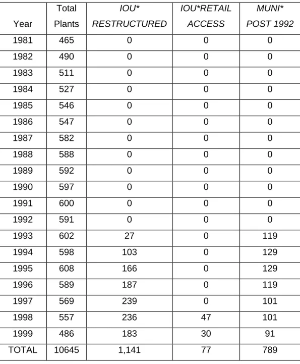
legislation.31 A second variable, RETAIL ACCESS, indicates the start of retail access for plants in the four states that implemented retail competition during the sample.32 Table 1 reports the
number of plants in our database each year that were in states that had RESTRUCTURED and the
29 In a 1993 article outlining PECO’s cost saving accomplishments and strategies for the future, Chairman
and CEO Joseph Paquette discussed restructuring of the utility industry and was quoted as stating, “we have been focusing on our strategic plans to enhance our abilities to satisfy our customer needs by becoming more competitive.” PECO initiatives cited in the article included improving the cost effectiveness of all operations. One particular accomplishment noted was the reduction in total employment from 18,700 to 12,900.
30 As noted earlier, some of these changes may have also affected utilities in non-restructuring states. For
example, the number of utility rate cases dropped dramatically in the 1990s, implying that many or most utilities may have been short- or medium-run residual claimants to cost reductions. Knittel (2002)
identifies a number of incentive regulations adopted in various jurisdictions during the 1990s. Many of the fuel-related regulations (modified pass-through clauses, heat rate and equivalent availability factor
incentive programs) were strongly correlated with ultimate restructuring. Some of the broader regulations (e.g., price caps and revenue decoupling programs) were almost orthogonal to eventual restructuring.
31 The RESTRUCTURED variable is based on whether a state had passed legislation as of mid-2001,
although in the aftermath of the California electricity crisis, there has been no additional restructuring, and some delays or suspension of planned restructuring activity.
32 While RESTRUCTURED indicates approval of retail access legislation, the specified phase-in of retail
access was often slow. Only five states implemented retail access during our sample period: Rhode Island in 1997, California, Massachusetts, and New York in 1998, and Pennsylvania in 1999 (U.S. EIA, 2003). Because we have no valid observations on Rhode Island plants in 1997 or beyond, retail access effects will be determined by the 4 states implementing in 1998 or 1999. Divestiture requirements in California and Massachusetts further reduces the post-retail access sample of plants, as investor-owned plants in those states were largely divested by 1999.
number of plants in states that had started retail access by 1999.33 If utilities did not respond until
restructuring legislation or regulation was enacted and the policy uncertainty resolved,
RESTRUCTURED will underestimate the true effect by averaging in non-response years. To
evaluate this possibility we introduce a third variable, LAW PASSED, an indicator equal to one beginning in the year the state passes restructuring legislation.34 Similarly if actual
implementation of retail access and the associated wholesale market reforms is important to efficiency gains, it will be reflected in an incremental effect of RETAIL ACCESS. To examine municipally-owned plants over the restructuring time period, we define the variable MUNI*POST
1992, equal to one for all municipally-owned plants from 1993, the first year for which RESTRUCTURED is one, through 1999. The final column reports the number of plants in this
category.
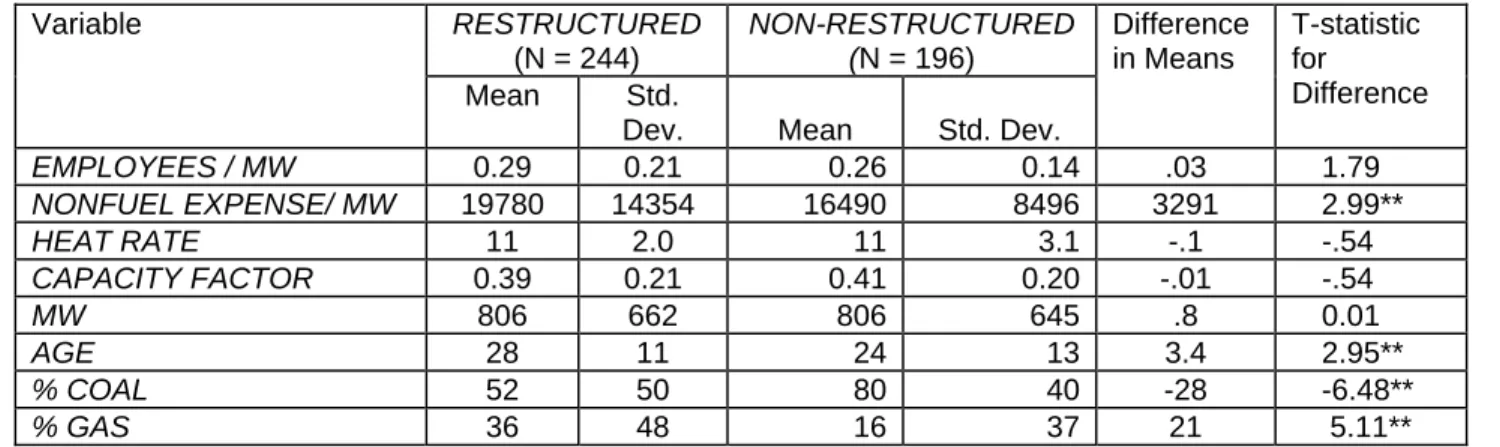
Details on the data sources and summary statistics are provided in the appendix. Tables 2a and 2b report summary statistics for plant-level data in 1985 across three categories: investor-owned plants in states that later restructure, investor-owned plants in states that do not restructure, and non-IOU plants. We choose this date to ensure that comparisons are made prior to any significant changes across states in the competitive or regulatory environment, even prior to restructuring initiatives. From these tables, it appears that the plants from these groups are not random draws from the same population. The first three variables measure employees and non-fuel operating expenses, scaled by the plant’s capacity, and fuel use in millions of British thermal units
(mmBtus), scaled by the plant’s output. In 1985, before state-level restructuring initiatives were considered, plants in states that eventually restructured had higher intensities of employees and non-fuel operating expenses, although the difference is significant only for non-fuel expenses. The first two rows in Table 2b show that municipally-owned plants had significantly higher employment and non-fuel input use than plants in non-restructuring states. The differences in heat rates and capacity factors are not significant in either of the tables. The last four variables in both tables describe the stock of plants in the two types of states. Although plants are very similar in size across IOUs, MUNIs plants are considerably smaller. IOU plants in restructuring
33 For the tables and the regression analysis that follows, plants are assigned to the state in which they are
regulated. A plant located in one state may be owned by a company with exclusive service territory in a different state, and that second state is the state by which the regulatory policy is measured. Some plants are owned by a company with service territory in more than one state and some plants are owned by several companies that are regulated by different states. In the regression analysis, we found that separately characterizing “mixed” regulation and “shared” plants had very little impact on our results.
34 There is on average about a 2.6-year lag between the initiation of hearings and the passage of the law.
We have experimented with a number of alternative measures of restructuring activity, including variables that begin with hearings regardless of restructuring outcomes, those that measure years since hearings were
states tended to be older, more likely to use gas, and less likely to use coal, than IOU plants in non-restructuring states. MUNI plants tended to be younger, less likely to use coal, and more likely to use gas, than IOU plants in non-restructuring states. The regression analysis will control for these differences directly or with the use of plant-epoch effects.
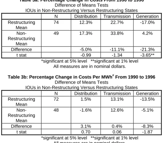
If investor-owned utilities achieved efficiency improvements when facing impending
restructuring of the generation sector, one would expect to see a relative decrease in the cost of generation for affected companies, and little difference in the change in transmission and distribution costs between the affected and not affected states since restructuring programs leave transmission and distribution comparatively untouched. If restructuring did not affect operating efficiency in the generation sector, we might expect either (1) the change in generation expenses would not be statistically different between restructuring and non-restructuring companies, or (2) we would see the same pattern of change in costs for the transmission and distribution sectors as for the generation sector.35
Table 3a and 3b display the difference in mean tests for investor-owned utilities in restructuring and non-restructuring states for a change in costs between 1990 and 1996. Table 3a reports the percentage change in total costs for each category of cost, and Table 3b reports the percentage change in costs per MWh. The larger decrease in generation costs at restructuring companies is significant at the 1% level, and the result for generation costs per MWh is significant at the 6% level. The difference in costs for companies in restructuring and non-restructuring states is not significant for either the transmission or distribution costs. These aggregate statistics provide preliminary support for the expectation that the portion of the utility company faced with competition (the generating sector) responded with a decrease in costs, while other sectors and companies not faced with competition did not share this response.
4. The Effects of Restructuring on Input Use
initiated for states that eventually restructured, and the presence of restructuring-associated rate freezes. None of these seem to change materially to the conclusions we draw below.
35 For the analysis comparing costs of generation, transmission, and distribution services, we rely on data
reported annually by utility companies to the Federal Energy Regulatory Commission (FERC) in the FERC Form 1, page 320, 321, and 322 respectively. We use a balanced sample composed of all companies with data reported for all three sectors in both 1990 and 1996. This amounts to 49 companies in states that did not deregulate and 74 in states that did deregulate for the comparison of costs, and 48 and 72 respectively for the comparison of costs per MWh. Using costs per MWh necessitates the exclusion of a few companies for which MWh data was not available in one of the two years.
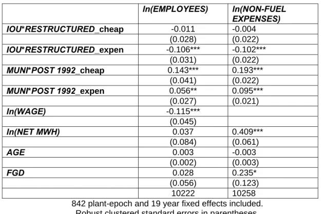
Following equation (I1), we estimate the influence of restructuring on the use of input N (EMPLOYEES, NONFUEL EXPENSE, and BTUs) with the following basic regression model:
(R1) ln(Nirt) = β1Nln(NET MWhirt) + β2Nln(PRICENrt ) + β3kAGEirt + β4kFGDirt +
φ r NIOU*RESTRUCTURED + γMUNI1993-1999 + αiN + δtN + β1Nε irt A + ε ir tN
where we allow for non-unity coefficients on the output term (β1N ) for all equations and on the
input price term (β2N on WAGE) in the EMPLOYEES equation,36 and include controls for two
important plant characteristics that vary over time: AGE and FGD (scrubber). αiN is a
time-invariant fixed effect for input N at plant-epoch i, which may contain a state-specific and ownership-specific error that will not be separately identified. These plant-specific effects control for much of the expected variation in input use across plants arising from heterogeneous technologies, state or regional fixed factors, and basic efficiency differences. They also control for differences in the plant mix between restructuring and non-restructuring states by comparing each plant to itself over time, removing any time-invariant plant effects. As a Hausman test rejects the exogeneity of plant effects, all reported results include plant-epoch fixed-effects.37 δ
tN
is an industry-level effect in year t, which controls for systematic changes in input demand across all plants over time.
εirtN is assumed to be a time varying mean zero shock for input N at plant-epoch i in regime r at
time t. This shock is unlikely to be independent over time for a given plant. There is likely to be persistence in input shocks, particularly for labor, from year to year. Indeed, estimated rhos based on assumed first-order serial correlation are in the .65 range for labor inputs and in the .33 range for non-fuel expenses. It is unlikely that the correlation is as simple as a first-order autogressive process, however. The physical operation of power plants is likely to induce some correlation at longer differences. For example, routine maintenance cycles may involve
scheduled shutdowns but increased labor and nonfuel expenses every three or four years. We have explored GLS specifications based on an assumption of first-order autoregressive errors, and the results are quite similar to those reported in the tables below. Rather than impose this
assumption, however, we choose to estimate the model without a GLS correction, and simply
36 Recall that we do not have a price associated with nonfuel expenses, and that according to equation (E1),
fuel prices should not enter into the fuel input function. We experimented with using a variable measuring the price of a given plant’s fuel relative to the prices of other fuels in the same region as an instrument for output but the variable had no power in the first stage.
37 This use of fixed effects is similar to the work of Joskow and Schmalensee (1987), who used generating
report standard errors that are corrected for a general pattern of correlation over time within a given plant.38
Input use over time will vary with the level of plant operation, which is measured in these specifications as the net generation by the plant in megawatt-hours (NET MWh). We treat the endogeneity and measurement problems described earlier by instrumenting for output with state demand (the log of total state electricity sales, a consumption rather than production measure). This instrument affects the likelihood that a given plant in the state will be dispatched more over the year, but is not influenced by the characteristics of the plant or the choices of individual plant operators.
We consider specifications that include interactions of IOU ownership with the three primary restructuring indicator variables described in section 3: RESTRUCTURED, LAW PASSED, and
RETAIL ACCESS. In the input regressions, a negative coefficient on the restructuring variables
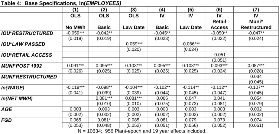
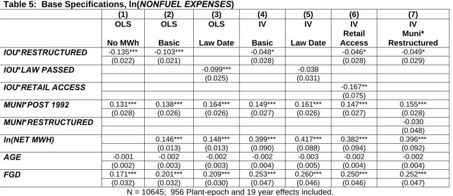
would imply increased input efficiency associated with the regulatory reform. The core results for the input analysis are presented in Tables 4 for EMPLOYEES, 5 for NONFUEL EXPENSES and 6 for BTU. We first discuss the results for employment and nonfuel expenses, and then discuss the results for fuel use.
Column 1 of tables 4 and 5 reports a simple OLS formulation that excludes any control for output. In this column, IOU*RESTRUCTURED captures the mean differential in input use for investor-owned plants in states that eventually pass restructuring legislation, measured over the period following the first restructuring hearings, relative to IOU plants in non-restructuring states. This corresponds to the mean within-plant shift in input use, independent of output. The results suggest statistically and economically significant declines in inputs during restructuring. Employment declines by almost 6% (2%) and nonfuel expenses decline by almost 13% (2%),39
relative to IOU plants in regimes that have not restructured. Controlling for plant output reduces the estimated impact of restructuring by more than one-quarter, though the effects remain large and statistically distinguishable from zero (see column 2 of each table), at -4% (2%) for employment and -10% (2%) for nonfuel expenses.40 Measuring restructuring effects from the
fixed effects are actually finer than plant-level, as we permit αi to change with unit additions or retirements
and other significant changes in rated plant capacity.
38 Reported standard errors are calculated using the cluster option in Stata. 39 We use [exp(φ
r N )-1]*100 to approximate the implied percentage effect of IOU* RESTRUCTURED on
input use.
40 Note that the Cobb-Douglas functional form assumption suggests that the coefficient on output should be
one, substantially larger than the coefficients estimated in these regressions. If we impose this constraint, the effect of restructuring is estimated to be positive and significant. We have estimated production
enactment date of legislation does little to change the qualitative conclusions (see column 3 in each table.).
This finding hints at an interesting pattern in the data: restructuring is associated with same-plant output reductions relative to same-plant output in non-restructured regimes at the same date. This is why estimated input use reductions associated with restructuring are smaller in the presence of output controls. Some of this might be expected: if these plants were less efficient prior to restructuring, as the raw input and price data suggest may have been the case, they may be used less in a more competitive environment. If restructuring encourages entry by non-utility or exempt generators, this might further reduce output at less efficient plants.41 Some plant-level
output reduction also may be generated by the apparent lower growth in state-level electricity consumption in restructuring states, relative to electricity consumption growth in
non-restructuring states.42
This result is not only of interest economically, but also is important for the econometric estimation of the input demand relationship. The inverse correlation of output and restructuring policy attaches great importance to obtaining a consistent estimate of the relationship between output and input demand. Understating the response of input use to output changes will load more of observed input reductions onto the restructuring variable, overstating the responsiveness will lead to underestimates of the restructuring effect.
The second notable pattern is the dependence of the implied restructuring effect on the control group. While IOU plants in restructuring states exhibit modest reductions in employment and nonfuel expenses relative to IOUs in non-restructuring states, the implied reductions are more than twice as large when compared to public and cooperative plants over the restructuring period. Employment drops by 13-15 percent (see the difference in the IOU*RESTRUCTURED and
MUNI*POST 1992 coefficients in columns 2 and 3 in table 4) and nonfuel expenses decline by
21-23 percent (columns 2 and 3 in table 5), relative to municipal plants over the 1993-1999
functions in EMPLOYEES and NON-FUEL EXPENSES using more flexible functional forms than Cobb-Douglas, and the results also suggest efficiency gains associated with restructuring. We have also
estimated instrumental variables versions of equations (L2) and (M2) that include the other input instead of output and obtained very similar results to those reported here.
41Total state-level electricity consumption, while increasing on average during the 1993-1999 period in
restructuring states, appears to grow less fast than consumption in non-restructuring states.
42 This is unlikely to be causally related to restructuring, as restructuring effects on retail rates were neutral
or negative (due to rate freezes) during this period. There is, however, a negative correlation between state electricity consumption and restructuring, conditioning on state means and national growth rates in electricity consumption.