Secular Variation of the Intensity of the Geomagnetic Field in Mexico During the First Millennium BCE

(1)

HAL Id: hal-02373176

https://hal.archives-ouvertes.fr/hal-02373176

Submitted on 26 Nov 2019

HAL is a multi-disciplinary open access

archive for the deposit and dissemination of

sci-entific research documents, whether they are

pub-lished or not. The documents may come from

teaching and research institutions in France or

abroad, or from public or private research centers.

L’archive ouverte pluridisciplinaire HAL, est

destinée au dépôt et à la diffusion de documents

scientifiques de niveau recherche, publiés ou non,

émanant des établissements d’enseignement et de

recherche français ou étrangers, des laboratoires

publics ou privés.

G. Hervé, Mireille Perrin, Luis Alva-Valdivia, Alejandro Rodriguez-Trejo,

Arnaldo Hernandez-Cardona, Mario Cordova Tello, Carolina Meza Rodriguez

To cite this version:

G. Hervé, Mireille Perrin, Luis Alva-Valdivia, Alejandro Rodriguez-Trejo, Arnaldo

Hernandez-Cardona, et al.. Secular Variation of the Intensity of the Geomagnetic Field in Mexico During the

First Millennium BCE. Geochemistry, Geophysics, Geosystems, AGU and the Geochemical Society,

2019, 20 (12), pp.6066-6077. �10.1029/2019GC008668�. �hal-02373176�

(2)

Secular Variation of the Intensity of the Geomagnetic

Field in Mexico During the First Millennium BCE

Gwenaël Q2

Q3

Hervé1 ,MireillePerrin1 ,Luis M.Alva‐Valdivia2,AlejandroRodriguez‐Trejo2,

ArnaldoHernandez‐Cardona2,MarioCórdova Tello3, andCarolinaMeza Rodriguez3

1_{Aix Marseille University, CNRS, IRD, INRA, Coll France, CEREGE, Aix}_{‐en‐Provence, France,}2_{Instituto de Geofísica,}

Laboratorio de Paleomagnetismo, Universidad Nacional Autónoma de México, Mexico City, Mexico,3_{Instituto Nacional}

de Antropologia e Historia, Centro Morelos, Mexico

Abstract

In Western Eurasia, thefirst millennium BCE is characterized by the fastest secular variation of the Earth Magnetic Field observed over the last millennia and by a geomagnetic anomaly centered on the Middle East. On the global scale, the variation of the dipolarfield during this period remains poorly constrained because of the lack of data in other geographical areas. Here, we presented 23 new mean archaeointensity data on ceramic sherds dated between 1500 BCE and 200 CE from Chalcatzingo archaeological site in Central Mexico. Archaeointensities were determined using the classical Thellier‐ Thellier protocol with corrections for TRM anisotropy and cooling rate effects. Our work doubles the number of high‐quality archaeointensity data in Mexico during the considered period. Using a Bayesian approach, a new secular variation curve was calculated at Mexico City between 1500 BCE and 200 CE after selection of Mexican archaeointensity data. After a period of oscillations of the intensity between 20 and 40μT from 1500 to 300 BCE, the curve shows a large maximum `~65 μT in the second century BCE. The corresponding VADM varied between ~4.0 and ~11.0 × 1022Am2, which highlights further that the intensity of the geomagneticfield could vary at regional scale over a larger range as previously thought. However, this amplitude variation may be overestimated, as it does not take into account the fast directional variation observed at this time.

Plain Language Summary

Archaeological baked clays are the best material to reconstitute the past secular variation of the Earth magneticﬁeld, because they acquired a generally stable

thermoremanent magnetization usually parallel and proportional to the ambientfield at the time of their baking. Global modeling of the geomagneticfield requires a spatial and temporal distribution of data as homogeneous as possible, which is still not the case yet. In spite of its rich archaeological heritage, high‐ quality archaeointensity data are still very few in Mexico. The present study focuses on pottery sherds dated between 1500 BCE and 200 CE from Chalcatzingo archaeological site in Central Mexico. We obtained 21 new mean archaeointensities, which almost doubles the high‐quality Mexican dataset for this period. The new secular variation Mexican curve exhibits oscillations of the intensity between 20 and 40μT from 1500 to 300 BCE, before a large maximum ~65μT in the second century BCE. This work will help to have a better knowledge of the variation of the dipolar geomagneticfield during the first millennium BCE, when the fastest secular variation over the last millennia was reported in the Middle East (“geomagnetic spikes”).

1. Introduction

Knowing how the geomagneticfield changed through time is crucial to understand the functioning of the geodynamo and theflux dynamic in the Earth's core. Beyond the last centuries, absolute but discrete estima-tions of the past geomagnetic direction and intensity are recovered from volcanic lavaflows and archaeolo-gical baked clays. Lacustrine and marine sediments can also be used, but these continuous records provide only relative data that tend to smooth the secular variation of the geomagneticfield. Global models of the field during the Holocene were developed by inversion of absolute and/or relative data using spherical har-monic analysis in space (e.g., Arneitz et al., 2019; Constable et al., 2016; Hellio & Gillet, 2018; Pavón‐ Carrasco et al., 2014).

In spite of important improvements in the past 10 years, the accuracy of the models is still weakened by the inhomogeneous spatial distribution of worldwide data with around 70% of the data concentrated around ©2019. American Geophysical Union.

RESEARCH ARTICLE

10.1029/2019GC008668

Key Points:

• Twenty‐three new archaeointensity data were obtained on pottery sherds from Central Mexico in theﬁrst millennium BCE

• A new Mexican secular variation curve between 1500 BCE and 200 CE is proposed

• The curve exhibits a fast increase of the intensity (~250 nT/year) during the third century BCE and a large maximum ~65μT circa 200–100 BCE Supporting Information: • Supporting Information S1 • Supporting Information S2 Correspondence to: G. Hervé, gwenael.herve@u‐bordeaux‐mon-taigne.fr Citation:

Hervé, G., Perrin, M., Alva‐Valdivia, L. M., Rodriguez‐Trejo, A., Hernandez‐ Cardona, A., Tello, M. C., & Rodriguez, C. M. (2019). Secular variation of the intensity of the geomagneticﬁeld in Mexico during theﬁrst millennium BCE. Geochemistry, Geophysics, Geosystems, 20. https://doi.org/10.1029/ 2019GC008668 Received 30 AUG 2019 Accepted 19 OCT 2019 Q4 2 3 4 5 6 7 8 9 10 11 12 13 14 15 16 17 18 19 20 21 22 23 24 25 26 27 28 29 30 31 32 33 34 35 36 37 38 39 40 41 42 43 44 45 46 47 48 49 50 51 52 53 54 55 56 57 58 59 60 61 62 63 64 65

(3)

Western Eurasia (Brown et al., 2015). The temporal resolution of the archaeomagnetic records is lower in other regions, such as in Asia (e.g., Cai et al., 2016, 2016), Oceania (e.g., Greve & Turner, 2017), and Northern America (e.g., Hagstrum & Champion, 2002; Lengyel, 2010). One of the main consequences is the poor knowledge of dipole moment variation prior to 1840. Models disagree when to know if the dipole moment decreased regularly since ~750 CE (Poletti et al., 2018) or since ~1700 CE after seven centuries of stability (Hellio & Gillet, 2018). The lack of data also prevents a precise understanding of geomagnetic anomalies at the Earth's surface such as the present South Atlantic anomaly (e.g., Campuzano et al., 2019; Terra‐Nova et al., 2017).

Another geomagnetic anomaly centered on the Middle East has recently been proposed at the beginning of thefirst millennium BCE (Shaar et al., 2016; Shaar et al., 2017). This Levantine Iron Age anomaly (LIAA) was likely at the origin of two short‐lived high‐intensity events called “geomagnetic spikes” (Ben‐Yosef et al., 2009; Shaar et al., 2011). The migration of the LIAA through Europe would be responsible for the large and fast variations of the geomagneticfield observed in this region during the first millennium BCE in both direction (e.g., Hervé et al., 2013; Palencia‐Ortas et al., 2017; Shaar et al., 2018) and intensity (e.g., Hervé et al., 2017; Molina‐Cardin et al., 2018; Shaar et al., 2016). Besides the role of these nondipolar fields, global reconstructions of data suggest that the influence of the dipolar field should not be underestimated with a maximum of the dipole moment during thefirst millennium BCE (Usoskin et al., 2016) and a 10–15° dipole tilt during thefirst half of this millennium (Nilsson et al., 2010). But the knowledge of the respective contri-butions of different harmonic degrees to the secular variation during thefirst millennium BCE remains hampered by the lack of data outside Western Eurasia.

In this context, Mexico is a key area to explore the secular variation at low latitudes, thanks to its rich archae-ological heritage at this time linked to the powerful Olmec civilization. Mexico is also close to Hall's cave in Texas, where a“geomagnetic spike” seems to exist in two sedimentary sequences at the beginning of the first millennium BCE (Bourne et al., 2016). No absolute data have confirmed this “spike” for the moment. In Mexico, a large number of archaeomagnetic studies on baked clays or lavaflows have been published in the last 10 years (e.g., Fanjat et al., 2013; Mahgoub et al., 2017; Mahgoub et al., 2019; Mahgoub et al., 2019; Pétronille et al., 2012; Rodriguez‐Ceja et al., 2009; Rodriguez‐Trejo et al., 2019; Terán et al., 2016), but a recent critical analysis of the Mexican dataset (Hervé et al., 2019) showed that around 70% of these data cannot be considered as high quality, according to basic selection criteria. Two local secular variation curves have been recently proposed using only Mexican data (Mahgoub, Juarez‐Arriaga, et al., 2019) or also some from the southwestern United States (Goguitchaichvili et al., 2018). The significant differences between the two curves point out that the resolution of the secular variation during thefirst millennium BCE is still not good. High‐quality data are especially lacking between 1500 and 400 BCE and the present study, with 23 new archaeointensities from Chalcatzingo in Central Mexico, doubles the database.

2. Archaeological Context and Sampling

The archaeological site of Chalcatzingo (lat: 18.6766°N, long: 98.7705°W) is located above the fertile Amatzinac valley in the Morelos state at circa 120 km southeast of Mexico City (Figures 1a and 1b).F1

Excavations, carried out since the 30 s, are presently directed by Mario Córdova Tello and Carolina Meza Rodriguez from the Instituto Nacional de Antropologia e Historia (INAH).

Chalcatzingo was an important regional center in Central Mexico between 1500 and 500 BCE at the Preclassic period. The site was organized in terraces at the base of two volcanic peaks called Cerro Chalcatzingo and Cerro Delgado (Grove, 1987). The remains highlighted an increasing political organization and the development of long‐distance trade, especially with the Gulf coast of Mexico that was the heartland of the Olmec civilization at this period. Famous ritual petroglyphs of Chalcatzingo are the most significant witnesses of the Olmec influence in Central Mexico (Cordova Tello & Meza Rodriguez, 2017; Cyphers Guillen, 1982). The stratigraphy divided the occupation in three successive phases, called Amate (~1500 to ~1100 BCE), Barranca (~1100 to ~700 BCE), and Cantera (~700 to ~500 BCE). Each phase was defined by specific pottery types. This relative chronology was fixed to the calendar scale through 57 radiocarbon dates (Cyphers Guillen & Grove, 1987).

5 6 7 8 9 10 11 12 13 14 15 16 17 18 19 20 21 22 23 24 25 26 27 28 29 30 31 32 33 34 35 36 37 38 39 40 41 42 43 44 45 46 47 48 49 50 51 52 53 54 55 56 57 58 59 60 61 62 63 64 65

(4)

After a peak during the Cantera phase, the site rapidly declined in the Late Preclassic period (400 BCE to 200 CE) but remained inhabited during Classic (200–650 CE), Epiclassic (650–900 CE), and Postclassic (900– 1500 CE) periods. Thirteen archaeointensity data from Epiclassic potteries have already been published (Hervé, Chauvin, et al., 2019). Here we focused on Preclassic sherds.

We collected 44 fragments of pots that were discovered in the Terrace 6 “the hunter” or close to the Monument 19 (Table S1 in the supporting information). Pots belong to nine types of pottery: Tenango cafe,

Cuautla rojo, and Cuautla cafe for the Amate phase; Blanco Amatzinac,

Anaranjado peralta, Laca, and Imitacion Laca for the Barranca phase;

Atoyac pulido con engobefor the Cantera phase; and Cajete concavo abierto for the Late Preclassic phase. We preferentially sampled these types because they are, at least partly, red‐colored (Figure 1c). Archaeointensity experiments are generally more successful on these pot-teries than on the grey‐black one, because they are less sensitive to miner-alogical alteration (Osete et al., 2016).

3. Archaeomagnetic Experiments

3.1. Rock Magnetism

To investigate the ferromagnetic mineralogy, thermomagnetic curves were measured on powders from nine sherds, one from each pottery type, using the Agico MFK1 apparatus in the CEREGE laboratory. The varia-tion of the susceptibility was measured during heating to 450 or 620°C and subsequent cooling. Backﬁeld curves of an isothermal remanent magnetization (IRM) from a 1 T mag-neticﬁeld were acquired on chips from the same sherds with Princeton Micromag Vibrating Sampling Magnetometer at CEREGE.

3.2. Archaeointensity Study

Archaeointensity experiments were performed using the classical Thellier‐Thellier method (Thellier & Thellier, 1959) on 135 specimens. Sherds were cut in 0.1 to 4.3 g chips that were embedded in 2 cm cubes of nonmagnetic plaster. Specimens were heated in an ASC TD48‐SC furnace with a 30 or 40 μT laboratory ﬁeld. Up to 12 temperature steps were performed between 100 and 620°C. Partial thermoremanent magne-tization (pTRM) checks every two steps monitored the absence of alteration of the ferromagnetic mineral-ogy. After each step, remanent magnetizations were measured with a SQUID cryogenic magnetometer (2G Enterprises, model 755R).

For potteries, it is well known that the correction of TRM anisotropy is crucial (Veitch et al., 1984). The most reliable method is the correction by the tensor of TRM anisotropy. The tensor was determined at the speci-men level at 530–560°C using six positions (+x, −x, +y, −y, +z, and −z axes) followed by a stability check (Chauvin et al., 2000). The correction was not applied if the difference between the PTRM moments of theﬁrst and seventh steps exceeded 10%.

The TRM intensity also depends on the cooling duration, and many archaeointensity studies on baked clays have demonstrated the necessity to correct this cooling rate effect, when the duration of the initial and laboratory cooling is significantly different (e.g., Fox & Aitken, 1980; Hervé et al., 2019). In this study, the cooling of the specimens in the laboratory furnace lasted about 30 min that is much faster than the archae-ological cooling. To correct for this effect, the procedure of Gómez‐Paccard et al. (2006) was carried out with a slow cooling over 5 hr at the same temperature that the one of the anisotropy correction. This approxima-tion of the archaeological cooling may not be very accurate and was defined mainly for technical reasons. If we cannot totally discard an effect of this possible underestimation of the archaeological cooling on the archaeointensity determinations, it was shown that the TRM intensity increases with the cooling duration following a logarithmic trend (e.g., Genevey et al., 2008; Halgedahl et al., 1980). Hervé, Perrin, et al. (2019) demonstrated that such imprecision on the cooling estimation does not result in a significant

Figure 1. (a) General view and (b) location of Chalcatzingo archaeological

site. In (c) are shown representative Preclassic pots of Blanco Amatzinac (no. 16), Anaranjado peralta (no. 20), and Cajete concavo abierto (no. 50) types. 5 6 7 8 9 10 11 12 13 14 15 16 17 18 19 20 21 22 23 24 25 26 27 28 29 30 31 32 33 34 35 36 37 38 39 40 41 42 43 44 45 46 47 48 49 50 51 52 53 54 55 56 57 58 59 60 61 62 63 64 65

(5)

inaccuracy of the average archaeointensity. Furthermore, much slower values of cooling rate are not expected at this archaeological period.

4. Results

4.1. Rock Magnetism

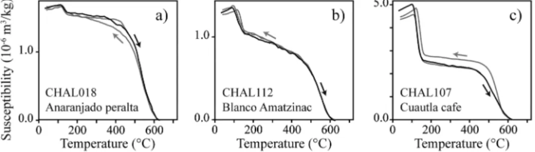
Susceptibility curves acquired during successive heating and cooling of the samples (thermomagnetic curves) present a good within 10% reversibility (Figure 2), which highlighted the suitability ofF2

Chalcatzingo sherds for archaeointensity experiments. All curves show a ferromagnetic carrier with Curie temperature close to 585°C identiﬁed as almost pure magnetite. A second carrier with a Curie temperature around 130–150°C is also seen. This phase represents only a few per cent of the susceptibility in Anaranjado

peralta, Atoyac pulido con engobe, and Cajete concavo abierto types (Figure 2a), around 10–20% in Tenango cafe, Cuautla rojo, and Blanco Amatzinac types (Figure 2b) and up to 40–60% in Cuautla cafe, Laca, and Imitacion Lacatypes (Figure 2c). The low Curie temperature could correspond to a Ti‐rich titanomagnetite

or to an epsilon iron oxide (ε‐Fe2O3) (Lopez‐Sanchez et al., 2017). Backﬁeld curves are used to make the

dif-ference between the two possibilities. The curves of all specimens are close to saturation at 300 mT magne-tization (Figure3) and do not indicate a signiﬁcant contribution of high coercivity phases to the remanence.F3

These results exclude the presence of a high‐coercivity epsilon iron oxide. The low Curie temperature phase is likely a Ti‐rich titanomagnetite.

4.2. Archaeointensity Study

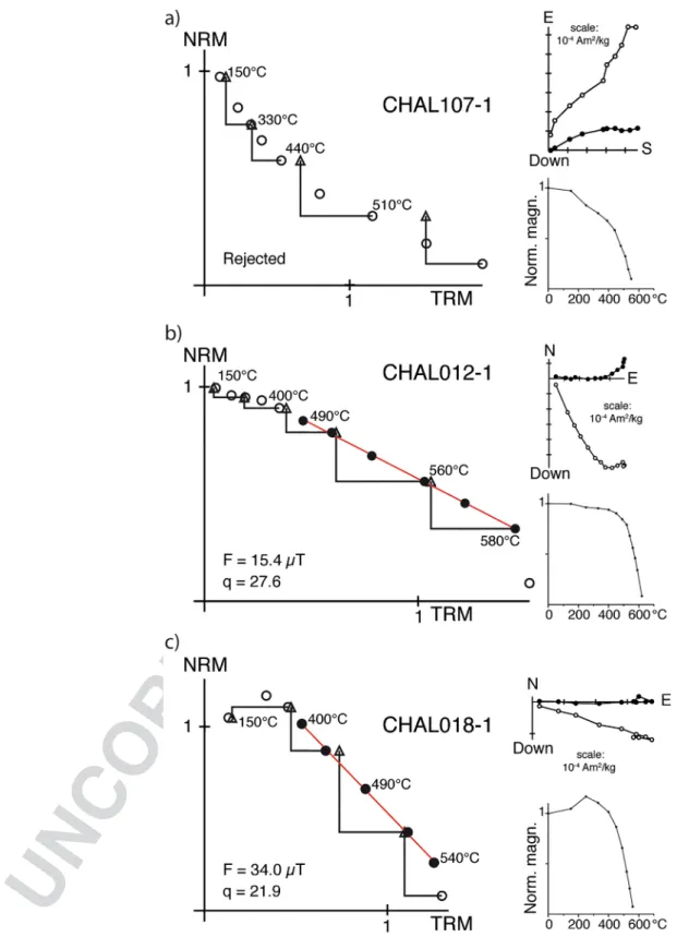
Most specimens show a secondary component of magnetization, removed between ~200 and ~500°C, that could have been acquired during the cooking use of the ceramic or after the excavation during the storage close to metallic shelves (Figure4). These specimens areF4

discarded when the characteristic remanent magnetization (ChRM) carries a fraction of the natural remanent magnetization (NRM) less than 35% (f factor), as in PICRIT‐03 (Kissel & Laj, 2004), SELCRIT2 (Biggin et al., 2007), and Thellier Tool TTA (Leonhardt et al., 2004) sets of selection criteria. Specimens are also rejected when they dis-play evidence of mineralogical changes on the temperature interval of the ChRM with negative pTRM checks and/or a concave‐up beha-vior (Figure 4a). Successful specimens, showing linear NRM‐TRM diagrams with positive pTRM‐checks (Figures 4b and 4c), have a quality factor (q) between 5 and 58 (Table S1). Around 80% of the spe-cimens have a maximum angular deviation (MAD) lower than 5°, a deviation angle (DANG) lower than 5°, and a ratio of the standard error of the slope to the absolute value of the slope (ß) lower than 0.05. The acceptance rate reaches 58% with 78 accepted specimens from 23 pots. Except for two pots (CHAL019 and CHAL132), at least three specimens are accepted per pot. No pots from Cuautla cafe,

Imitacion Lacatypes, and only one from Laca type provided a good

Figure 2. Representative thermomagnetic curves of Preclassic sherds from Chalcatzingo. The black curve is the variation

of susceptibility during the heating and the grey curve during the cooling.

Figure 3. Backﬁeld curves of isothermal remanent magnetization (IRM)

normal-ized to the IRM at 1 T. Samples with red, green and blue curves have thermo-magnetic curves showing respectively a low (<5%), medium (10–20%) and high (40–60%) proportion of the low‐Curie temperature phase.

5 6 7 8 9 10 11 12 13 14 15 16 17 18 19 20 21 22 23 24 25 26 27 28 29 30 31 32 33 34 35 36 37 38 39 40 41 42 43 44 45 46 47 48 49 50 51 52 53 54 55 56 57 58 59 60 61 62 63 64 65

(6)

Figure 4. (a) Rejected and (b and c) accepted archaeointensity results with NRM‐TRM diagrams on the left and

orthogo-nal plots and demagnetization curves on the right. The solid circles on NRM‐TRM diagrams indicate the temperature steps used in the intensity determination. On orthogonal plots, the open (solid) circles denote the projection on the vertical (horizontal) plane. 5 6 7 8 9 10 11 12 13 14 15 16 17 18 19 20 21 22 23 24 25 26 27 28 29 30 31 32 33 34 35 36 37 38 39 40 41 42 43 44 45 46 47 48 49 50 51 52 53 54 55 56 57 58 59 60 61 62 63 64 65

(7)

result. These three types have the largest Ti‐rich titanomagnetite content, suggesting that this magnetic carrier was likely the main responsible of the thermal instability.

The 23 new average archaeointensities have a good internal consistency with experimental uncertainty from 0.5 to 3.0μT (Table1). We do not observe a signiﬁcant difference between samples studied with 30 or 40 μT.T1

The uncertainty decreases after anisotropy and cooling rate corrections (see Table S1). The average values range between 15 and 43μT. No clear difference is observed between pots from the Terrace 6 and from the Monument 19. In the Barranca phase between 1100 and 700 BCE, pots from Blanco Amatzinac type pro-vide lower archaeointensities than those of Anaranjado peralta type, suggesting a noncontemporaneity of

these two types (Figure5a). F5

5. Discussion

5.1. Comparison With Other Mexican Data

A recent critical analysis of the Mexican intensity dataset showed that the data quality is unequal (Hervé, Chauvin, et al., 2019). In this study, the 194 available Mexican data were classiﬁed according to their cooling unit consistency and the quality of their palaeointensity protocol: (i) a number of specimens higher than three, (ii) a standard deviation lower than 15%, (iii) a palaeointensity acquired by Thellier‐Thellier or micro-wave protocols and calculated over a well‐deﬁned characteristic remanent magnetization, (iv) the presence of the cooling rate correction for archaeological baked clays, and (v) the presence of an anisotropy correction by the TRM tensor for generally anisotropic material such as potteries.

Over the 194 available in Mexico, only 14 data, eight from Duran et al. (2010), three from Rodriguez‐Ceja et al. (2009), and three from Rodriguez‐Ceja et al. (2012), fulﬁlled the quality criteria for the period between 2000 BCE and 200 CE. Intensities of Rodriguez‐Ceja et al. (2009, 2012) calculated on a secondary or two

Table 1

Average Archaeointensities

Date (years CE) Sherd Type of pottery Nacc/Nmeas FATRM+CR± SD (μT) FMexico City(μT) VADM (1022A.m2)

[‐1500; ‐1100] CHAL102 Tenango cafe 3/5 28.7 ± 1.7 29.0 6.5 ± 0.4

(Amate phase) CHAL103 Tenango cafe 3/4 37.7 ± 1.8 38.0 8.5 ± 0.4

CHAL104 Cuautla rojo 3/5 25.9 ± 0.7 26.1 5.9 ± 0.2

[‐1100; ‐700] CHAL012 Blanco Amatzinac 3/5 15.1 ± 0.5 15.2 3.4 ± 0.1

(Barranca phase) CHAL013 Blanco Amatzinac 4/4 29.5 ± 2.1 29.8 6.7 ± 0.5

CHAL015 Blanco Amatzinac 3/5 27.7 ± 1.6 27.9 6.3 ± 0.4

CHAL018 Anaranjado peralta 4/4 29.9 ± 2.6 30.2 6.8 ± 0.6

CHAL019 Anaranjado peralta 2/5 31.3 ± 2.5 31.6 7.1 ± 0.6

CHAL020 Anaranjado peralta 3/5 30.8 ± 2.5 31.1 7.0 ± 0.6 CHAL116 Anaranjado peralta 5/5 37.1 ± 3.0 37.4 8.4 ± 0.7

[‐1100; ‐600] CHAL117 Laca 4/4 26.9 ± 1.3 27.1 6.1 ± 0.3

(Barranca and

Cantara temprana phases)

[‐700; ‐500] CHAL126 Atoyac pulido 3/3 42.2 ± 1.2 42.6 9.5 ± 0.3

(Cantara phase) CHAL127 Atoyac pulido 3/4 38.0 ± 2.2 38.3 8.6 ± 0.5

CHAL128 Atoyac pulido 3/4 24.8 ± 2.0 25.0 5.6 ± 0.5

CHAL132 Atoyac pulido 2/4 31.1 ± 0.5 31.5 7.1 ± 0.1

[‐400; +200] CHAL050 Cajete concavo abierto 4/4 42.9 ± 2.1 43.3 9.7 ± 0.5 (Late Preclassic)

Note. Columns from left to right: date of the pottery type, sherd number, pottery type, number of accepted over measured specimens, average archaeointensity corrected for the effects of TRM anisotropy and cooling rate with its standard deviation, and average value relocated to Mexico City, Virtual Axial Dipole Moment. The two samples in italic are not taken into account in the calculation of the secular variation curve because the number of accepted specimens is lower than 3. 5 6 7 8 9 10 11 12 13 14 15 16 17 18 19 20 21 22 23 24 25 26 27 28 29 30 31 32 33 34 35 36 37 38 39 40 41 42 43 44 45 46 47 48 49 50 51 52 53 54 55 56 57 58 59 60 61 62 63 64 65

(8)

overlapping components of magnetization were not considered. Since the publication of Hervé, Chauvin, et al. (2019), the short high‐quality dataset was updated with four new data from Mahgoub, Juarez‐Arriaga, et al. (2019) and seven from Mahgoub, Juárez‐Arriaga, et al. (2019). Concerning our new Chalcatzingo data, 21/23 respect these criteria; the two sherds (CHAL019 and CHAL132) are discarded because only two successful archaeointensi-ties were obtained by sherd

Most other Mexican data were corrected for anisotropy effects with the Mean (XYZ) method, averaging the archaeointensities of six spe-cimens from the same sample, for which the laboratoryﬁeld during the Thellier experiments was applied along +x,−x, +y, −y, +z, or −z axis, respectively. As demonstrated by the experimental tests of Hervé, Chauvin, et al. (2019) and Poletti et al. (2016), this method leads to systematic larger imprecisions and to possible inaccuracies of more than 10μT. In Hervé, Chauvin, et al. (2019), we decided to retain such archaeointensities if they were calculated with six speci-mens, because the balanced participation of the three x, y, and z axes reduces the risk of inaccuracy. It is worth pointing out that this was a temporary solution, while waiting for publication of more archaeoin-tensity data corrected with the TRM tensor. Now that new data from Chalcatzingo and Mahgoub et al. (2019a, b) are available between 2000 BCE and 200 CE, we discard all data corrected with the Mean (XYZ) method.

On the Figure 5b, the 25 selected high‐quality Mexican data (listed in Table S2) are compared to the 21 new high‐quality Chalcatzingo data. All are relocated to Mexico City (19.4°N; 260.9°E) using the Virtual Axial Dipole Moment (VADM) correction. The new Chalcatzingo data almost doubled the number of high‐quality data between ~2000 BCE and ~200 CE and especiallyﬁlled up the temporal gap between 1000 and 400 BCE. They are consistent with the previously published ones.

Another drawback of the Mexican dataset is the imprecision of the archaeological chronology during the Preclassic period (from ~2000 BCE to ~200 CE) with phases (e.g., Amata, Barranca, and Cantara at Chalcatzingo) often covering several centuries. If the age of the boundaries between phases is relatively well controlled, thanks to radiocarbon dates, each phase is rarely subdivided on most sites as in Chalcatzingo. Therefore, there is a succession of wide time slices, in which the apparent dispersion of archaeointensity data, as between 1500 and 500 BCE, likely reflects the secular variation within this period. It makes more difficult the reconstitution of the secular variation with a high resolution. Another outstanding example is Cuanalan site dated between ~400 and ~100 BCE, for which the seven intensity values from Rodriguez‐Ceja et al. (2011) and Mahgoub, Juárez‐Arriaga, et al. (2019) range from ~25 to ~70μT, highlighting a fast increase of the geomagnetic field strength during the lifetime of the site.

5.2. Secular Variation Curve of the Intensity in Mexico Between 2000 BCE to 200 CE

From the selected dataset, we calculated a new secular variation curve with the same Bayesian framework (Lanos, 2004) as the one used in recent studies for Austria (Schnepp et al., 2015), Bulgaria (Kovacheva et al., 2014), France (Hervé & Lanos, 2018), and Hawaii (Tema et al., 2017). The inversion process takes into account experimental and age uncertainties on data and minimized the misﬁt of each data with the curve by exploring the multi‐dimensional space of probability densities using Monte Carlo Markov chains (MCMC). The secular variation is given as a smooth continuous curve obtained by averaging cubic splines. The degree

Figure 5. Secular variation of the intensity in Mexico between 2000 BCE and 200

CE. (a) All new Chalcatzingo data classiﬁed per pottery type. (b) Comparison of Chalcatzingo data with high‐quality data from Mexico and new secular variation curve plotted with its 68% and 95% conﬁdence envelope. All data are relocated at Mexico City. The grey shaded area highlights the period of the geomagnetic “spike” found in sediments of Hall's cave (Bourne et al., 2016).

5 6 7 8 9 10 11 12 13 14 15 16 17 18 19 20 21 22 23 24 25 26 27 28 29 30 31 32 33 34 35 36 37 38 39 40 41 42 43 44 45 46 47 48 49 50 51 52 53 54 55 56 57 58 59 60 61 62 63 64 65

(9)

of the smoothing/ﬁtting of the cubic spline function to the data is controlled by a “shrinkage” prior probabil-ity (Congdon, 2010). Here, the average curve with the 68% and 95% conﬁdence envelopes is calculated after 50,000 MCMC iterations (Figure 5b).

After a fast decrease from ~45 to ~25μT circa 1500 BCE, the average curve exhibits a succession of minima and maxima between 20 and 40μT until circa 300 BCE. Then the geomagnetic field strength increases rapidly during the third century BCE and reaches a high maximum close to 65μT in 150–100 BCE. The fol-lowing intensity decrease during thefirst centuries BCE and CE seems also rapid. The 150–100 BCE maxi-mum is constrained by three high‐quality data on potteries from Mahgoub, Juárez‐Arriaga, et al. (2019). The effect of a nonlinear TRM acquisition behavior (Selkin et al., 2007) was not tested in Mahgoub, Juárez‐ Arriaga, et al. (2019) but is likely not significant, because the laboratory field was close to the archaeointensity estimates.

The oscillatory behavior between 1500 and 300 BCE is the solution found by the modeling tofit the different intensity values observed between data dated in the same archaeological phase. Even though these intensity differences clearly point out that the intensity of geomagneticfield was not stable between 1500 and 300 BCE, one cannot exclude that some current oscillations, as maybe the 800 BCE minimum related to only CHAL012 Chalcatzingo data point, are a statistical artifact due to the specific distribution of ages in the data-set. New archaeomagnetic data with intermediate ages are required to confirm the limits of these small minima and maxima between 1500 and 300 BCE.

The present curve indicates a maximal secular variation rate of ~250 nT/year during the third century BCE. This rate isfive times faster than the average variation rate of 55 nT/year since 1900 CE at Mexico City (Thébault et al., 2015) but is similar to the fastest rate observed in Europe during the last 3,500 years (e.g., Genevey et al., 2016; Hervé et al., 2017). Our curve does not show any evidence for the “geo-magnetic spike” seen in 893±135 BCE in two sedimentary sequences of Hall's cave in Texas, only 1,200 km away from Mexico City (Bourne et al., 2016) (Figure 5b). Unlike palaeointensities higher than 100 μT, two data (CHAL102, this study; EB‐229, Mahgoub, Juárez‐Arriaga, et al., 2019) possibly point out an intensity low around 15–20 μT at the same period. These low values will have to be confirmed but already shows that the intensity of the geomagneticfield varied at the regional scale over a larger range than previously thought. Therefore, the hypothesis of Bourne et al. (2016) should be taken with caution, as the relative palaeointensity records from sediments are less reliable than the absolute estimations from archaeological baked clays.

5.3. Comparison With Mexican Master Curves and Global Geomagnetic Models

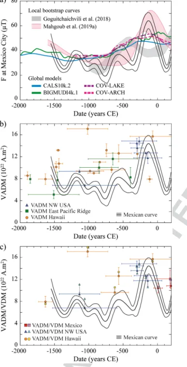
Two other secular variation curves of the intensity in Mexico have recently been published by Goguitchaichvili et al. (2018) and Mahgoub, Juarez‐Arriaga, et al. (2019), both calculated using a bootstrap approach (Thébault & Gallet, 2010) after different data selection (Figure6a). Mahgoub, Juarez‐Arriaga, et al.F6

(2019) curve differs by the inversion process based on the full geomagnetic vector taking into account direc-tional and intensity data at the same time. Whereas Mahgoub, Juarez‐Arriaga, et al. (2019) curve is close to our, although smoother, with an intensity maximum at the second century BCE, the curve of Goguitchaichvili et al. (2018) shows a minimum at this period. This inconsistency is likely related to the dif-ferences in the selection of the input dataset. Goguitchaichvili et al. (2018) study used a less up‐to‐date data-set with less stringent selection criteria, where data corrected with the Mean (XYZ) anisotropy method were also taken into account. In Mahgoub, Juarez‐Arriaga, et al. (2019) study, selection criteria are very similar to ours and all our selected data, except the new ones from Chalcatzingo, are included in their curve. The higher temporal resolution of our curve between 1500 and 500 BCE illustrates the impact of the Chalcatzingo data.

Contrary to our Bayesian curve, the predictions at Mexico City of the most recent geomagnetic global mod-els, BIGMUDI4k.1 (Arneitz et al., 2019), CALS10k.2 (Constable et al., 2016), COV‐ARCH, and COV‐LAKE (Hellio & Gillet, 2018), strongly smooth the secular variation (Figure 6a). Our Mexican curve is almost sys-tematically below the models between 1500 and 300 BCE. Models are also unable to reproduce the high‐ intensity maximum of the second century BCE. It is well known that these models, calculated using spheri-cal harmonic analysis, are limited by the uneven spatial and temporal distribution of the archaeomagnetic database (e.g., Brown et al., 2015). In Mexico, the unequal data quality also plays a major role (Hervé,

5 6 7 8 9 10 11 12 13 14 15 16 17 18 19 20 21 22 23 24 25 26 27 28 29 30 31 32 33 34 35 36 37 38 39 40 41 42 43 44 45 46 47 48 49 50 51 52 53 54 55 56 57 58 59 60 61 62 63 64 65

(10)

Chauvin, et al., 2019). The models were calculated using all Mexican data present in GEOMAGIA50.v3 database whatever their quality (Brown et al., 2015). Yet most low‐quality data, which were discarded in our local curve, were not adequately corrected for TRM anisotropy and cooling rate effects, which explains the smoothing of the varia-tion by the models and the tendency to overestimate the intensity between 1500 and 300 BCE (Hervé, Chauvin, et al., 2019).

5.4. Comparison With Other Regional Records

In Figure 6b, the secular variation curve of the Mexican VADMs, derived from our intensity curve, was compared to data from sur-rounding areas selected with the same selection criteria as the Mexican data. There are presently no high‐quality archaeointensities on archaeological baked clays in areas surrounding Mexico (southern United States, Central America, and northern South America). The closest are volcanic lava ﬂows from north‐western USA around 3000 km away from Mexico City (Champion, 1980) (Figure 6b). The East Paciﬁc ridge data on submarine basaltic glasses (Gee et al., 2000; Pick & Tauxe, 1993), located in the same longitudinal band at ~4,000–5,000 km off the coast of Peru, are also considered. Finally, we compare with the Hawaiian dataset ~6,000 km away at 55–60° of longitude (Cromwell et al., 2018; Tema et al., 2017). All selected data from the three regions are listed in Table S3.

While the VADMs from NW United States agree with the Mexican curve, the Hawaiian and East Pacific Ridge datasets show consis-tently higher values between 1000 and 300 BCE. This trend may indi-cate a nondipolar field feature close to Mexico during the first millennium BCE. Even though this hypothesis has clearly to be con-firmed by new high‐quality data from the Americas, it is interesting to note that CALS10k.2 model predicts a reverseflux patch of the radial component of the geomagnetic field at the core‐mantle boundary under Central America around 1000 BCE (Davies & Constable, 2017).

This discussion has also to take into account the fast directional variation observed in these regions during the first millennium BCE (e.g., Hagstrum & Champion, 2002; Tema et al., 2017). Actually, the Virtual Geomagnetic Poles derived from NW U.S. palaeodirections on lava flows were located up to ~70°N from ~60°E to ~0°E between 700 and 400 BCE. As the seven intensities that we selected from NW USA are also full vector, VDMs can be calculated in addition to the VADMs. VDMs are up to ~1.2 × 1022 A.m2 lower than the VADMs during the second half of the first millennium BCE and ~1.7 × 1022

A.m2higher between 1500 and 500 BCE (Figure 6c). The same trend is observed in the few full vector Hawaiian data. These differences between the VDMs and the VADMs minimize the amplitude of the secular variation of the VDM during theﬁrst millennium BCE in North America. The same observation is likely also valid for Mexico, where there are only three younger high‐quality full vector data from Mahgoub, Juarez‐Arriaga, et al. (2019) (Figure 6c). This clearly underlines the necessity of full vector determination for a good resolution of the secular variation of the Earth Magneticﬁeld.

Figure 6. (a) Comparison of the new secular variation curve with the previously

published local bootstrap curves for Mexico (Goguitchaichvili et al., 2018; Mahgoub, Juarez‐Arriaga, et al., 2019) and the predictions of global models BIGMUDI4k.1 (Arneitz et al., 2019), CALS10k.2 (Constable et al., 2016), COV‐ ARCH, and COV‐LAKE (Hellio & Gillet, 2018). (b) Comparison of the curve of the Virtual Axial Dipole Moment (VADM) in Mexico with data from north ‐wes-tern USA (Champion, 1980), the East Paciﬁc Ridge (Gee et al., 2000; Pick & Tauxe, 1993) and Hawaii (Cromwell et al., 2018; Mankinen & Champion, 1993; Pressling et al., 2006; Pressling et al., 2007; Tema et al., 2017; Valet et al., 1998). (c) Comparison of the VADMs with the Virtual Dipole Moments (VDMs) of full vector data from Mexico, Hawaii and north‐western USA.

5 6 7 8 9 10 11 12 13 14 15 16 17 18 19 20 21 22 23 24 25 26 27 28 29 30 31 32 33 34 35 36 37 38 39 40 41 42 43 44 45 46 47 48 49 50 51 52 53 54 55 56 57 58 59 60 61 62 63 64 65

(11)

6. Conclusion

The study of potteries from the archaeological site Chalcatzingo provides 23 new archaeointensity data for Mexico between 1500 BCE and 200 CE. Archaeointensities were determined using the classical Thellier‐ Thellier protocol with corrections for TRM anisotropy and cooling rate effects. With at least three specimens per pot, 21/23 data can be considered as high‐quality, which almost doubles the number of archaeointensity data in Mexico during the considered period.

Using a Bayesian framework, a new secular variation curve was calculated at Mexico City between 1500 BCE and 200 CE after selection of Mexican archaeointensity data. After a period of oscillations of the intensity between 20 and 40μT from 1500 to 300 BCE, the curve shows a large maximum ~65 μT in the second century BCE. The curve does not exhibit the“geomagnetic spike” seen in Texas (only ~1,200 km away from Mexico City) on relative sedimentary data at the beginning of theﬁrst millennium BCE. The corresponding VADM varied between ~4.0 and ~14.0 × 1022A.m2, but this variation amplitude would likely be lower if the direc-tional variation is considered. This highlights the critical need of full vector data in Mexico.

Our new dataﬁll a geographic gap in the global archaeomagnetic database between 1000 and 400 BCE, important to better reconstitute the variation of the dipolarﬁeld during this period in which “geomagnetic spikes” were reported in the Middle East. In this manner, the Levantine Iron Age anomaly can be better put in its general context.

Q5

References

Arneitz, P., Egli, R., Leonhardt, R., & Fabian, K. (2019). A Bayesian iterative geomagnetic model with universal data input: Self‐consistent spherical harmonic evolution for the geomagneticﬁeld over the last 4000 years. Physics of the Earth and Planetary Interiors, 290, 57–75. https://doi.org/10.1016/j.pepi.2019.03.008

Ben‐Yosef, E., Tauxe, L., Levy, T. E., Shaar, R., Ron, H., & Najjar, M. (2009). Geomagnetic intensity spike recorded in high resolution slag deposit in Southern Jordan. Earth and Planetary Science Letters, 287, 529–539. https://doi.org/10.1016/j.epsl.2009.09.001

Biggin, A. J., Perrin, M., & Dekkers, M. J. (2007). A reliable absolute palaeointensity determination obtained from a non‐ideal recorder. Earth and Planetary Science Letters, 257, 545–563. https://doi.org/10.1016/j.epsl.2007.03.017

Bourne, M. D., Feinberg, J. M., Stafford, T. W., Waters, M. R., Lundelius, E., & Forman, S. L. (2016). High‐intensity geomagnetic ﬁeld “spike” observed at ca. 3000 cal BP in Texas, USA. Earth Planet. Science Letters, 442, 80–92. https://doi.org/10.1016/j.epsl.2016.02.051 Brown, M. C., Donadini, F., Korte, M., Nilsson, A., Korhonen, K., Lodge, A., et al. (2015). GEOMAGIA50.v3: 1. General structure and

modiﬁcations to the archeological and volcanic database. Earth, Planets and Space, 67(1), 1–31. https://doi.org/10.1186/s40623‐015‐ 0232‐0

Cai, S., Jin, G., Tauxe, L., Deng, C., Qin, H., Pan, Y., & Zhu, R. (2016). Archaeointensity results spanning the past 6 kiloyears from eastern China and implications for extreme behaviors of the geomagneticﬁeld. Proceedings of the National Academy of Sciences. https://doi.org/ 10.1073/pnas.1616976114

Cai, S., Tauxe, L., Deng, C., Qin, H., Pan, Y., Jin, G., et al. (2016). New archaeomagnetic direction results from China and their constraints on paleosecular variation of the geomagneticﬁeld in Eastern Asia. Geophysical Journal International, 207, 1332–1342. https://doi.org/ 10.1093/gji/ggw351

Campuzano, S. A., Gómez‐Paccard, M., Pavón‐Carrasco, F. J., & Osete, M. L. (2019). Emergence and evolution of the South Atlantic Anomaly revealed by the new paleomagnetic reconstruction SHAWQ2k. Earth and Planetary Science Letters, 512, 17–26. https://doi.org/ 10.1016/j.epsl.2019.01.050

Champion, D.E., 1980. Holocene geomagnetic secular variation in the western United States: Implications for the global geomagneticﬁeld, U.S. Geophys. Res. Open File Rep., OF80‐824.

Chauvin, A., Garcia, Y., Lanos, P., & Laubenheimer, F. (2000). Paleointensity of the geomagneticﬁeld recovered on archaeomagnetic sites from France. Physics of the Earth and Planetary Interiors, 120, 111–136. https://doi.org/10.1016/s0031‐9201(00)00148‐5

Congdon, P. D. (2010). Applied Bayesian hierarchical methods. Boca Raton: Chapman an. ed.

Constable, C., Korte, M., & Panovska, S. (2016). Persistent high paleosecular variation activity in southern hemisphere for at least 10 000 years. Earth and Planetary Science Letters, 453, 78–86. https://doi.org/10.1016/j.epsl.2016.08.015

Cordova Tello, M., & Meza Rodriguez, C. (2017). Chalcatzingo, Morelos. Un discurso sobre piedra. Arqueologia Mexicana, 87, 60–65. Q6

Cromwell, G., Trusdell, F., Tauxe, L., & Ron, H. (2018). Holocene paleointensity of the Island of Hawaii from glassy volcanics. Geochemistry, Geophysics, Geosystems, 19, 3224–3245. https://doi.org/10.1002/2017gc006927

Cyphers Guillen, A. (1982). The implications of dated monumental art from Chalcatzingo, Morelos, Mexico. World Archaeology, 13, 382–393. https://doi.org/10.1080/00438243.1982.9979841

Cyphers Guillen, A., & Grove, D. C. (1987). Chronology and Cultural Phases at Chalcatzingo. In Ancient Chalcatzingo, (pp. 56–62). Davies, C., & Constable, C. (2017). Geomagnetic spikes on the core‐mantle boundary. Nature Communications, 8(1), 1–11. https://doi.org/

10.1038/ncomms15593

Duran, M. P., Goguitchaichvili, A., Morales, J., Aguilar Reyes, B., Alva Valdivia, L. M., Oliveros‐Morales, A., et al. (2010). Magnetic properties and archeointensity of Earth's magneticﬁeld recovered from El Openo, earliest funeral architecture known in Western Mesoamerica. Studia Geophysica et Geodaetica, 54, 575–593. https://doi.org/10.1007/s11200‐010‐0035‐5

Fanjat, G., Camps, P., Alva Valdivia, L. M., Sougrati, M. T., Cuevas‐Garcia, M., & Perrin, M. (2013). First archeointensity determinations on Maya incense burners from Palenque temples. Mexico: New data to constrain the Mesoamerica secular variation curve. Earth and Planetary Science Letters, 363, 168–180. https://doi.org/10.1016/j.epsl.2012.12.035

Fox, J. M. W., & Aitken, M. J. (1980). Cooling rate dependance of the thermoremanent magnetization. Nature, 283, 462–463. https://doi. org/10.1038/283462a0

Acknowledgments Funding was provided by ANR‐ CONACYT SVPIntMex project ANR‐ 15‐CE31‐0011‐01 coordinated by M. P. and L. A.‐V. G. H. also beneﬁted from a support of Campus France PRESTIGE program (PRESTIGE‐2017‐1‐0002). We are grateful to Gabrielle Hellio (University of Southampton) for trans-mitting the COV‐ARCH and COV‐ LAKE predictions at Mexico City and to Philippe Lanos for his help in the cal-culation of the Bayesian curve. We acknowledge Lisa Tauxe and an anon-ymous reviewer for their comments and corrections. Data at the site and speci-men levels are available on MagIC repository (https://earthref.org/MagIC/ 16700/d6c0ebb1‐43d8‐4c92‐a913‐ 45989e6b4f95). 5 6 7 8 9 10 11 12 13 14 15 16 17 18 19 20 21 22 23 24 25 26 27 28 29 30 31 32 33 34 35 36 37 38 39 40 41 42 43 44 45 46 47 48 49 50 51 52 53 54 55 56 57 58 59 60 61 62 63 64 65

(12)

Gee, J. S., Cande, S. C., Hildebrand, J. A., Donnelly, K., & Parker, R. L. (2000). Geomagnetic intensity variations over the past 780 kyr obtained from near‐seaﬂoor magnetic anomalies. Nature, 408(6814), 827–832. https://doi.org/10.1038/35048513

Genevey, A., Gallet, Y., Constable, C. G., Korte, M., & Hulot, G. (2008). Archeoint: An upgraded compilation of geomagneticﬁeld intensity data for the past ten millennia and its application to the recovery of the past dipole moment. Geochemistry, Geophysics, Geosystems, 9, Q04038. https://doi.org/10.1029/2007GC001881

Genevey, A., Gallet, Y., Jesset, S., Thébault, E., Bouillon, J., & Lefèvre, A. (2016). New archeointensity data from French Early Medieval pottery production (6th– 10th century AD). Tracing 1500 years of geomagnetic ﬁeld intensity variations in Western. Europe, 257, 205–219. https://doi.org/10.1016/j.pepi.2016.06.001

Goguitchaichvili, A., García, R., Pavón‐Carrasco, F. J., Julio, J., Contreras, M., María, A., et al. (2018). Last three millennia Earth's Magnetic ﬁeld strength in Mesoamerica and southern United States: Implications in geomagnetism and archaeology. Physics of the Earth and Planetary Interiors, 279, 79–91. https://doi.org/10.1016/j.pepi.2018.04.003

Gómez‐Paccard, M., Chauvin, A., Lanos, P., Thiriot, J., & Jiménez‐Castillo, P. (2006). Archeomagnetic study of seven contemporaneous kilns from Murcia (Spain). Physics of the Earth and Planetary Interiors, 157, 16–32. https://doi.org/10.1016/j.pepi.2006.03.001 Greve, A., & Turner, G. M. (2017). New and revised palaeomagnetic secular variation records from post‐ glacial volcanic materials in New

Zealand. Physics of the Earth and Planetary Interiors, 269, 1–17. https://doi.org/10.1016/j.pepi.2017.05.009 Grove, D. C. (1987). Ancient Chalcatzingo. Austin: University of Texas Press. 576 pp.

Hagstrum, J. T., & Champion, D. E. (2002). A Holocene paleosecular variation record from 14C‐dated volcanic rocks in western North America. Journal of Geophysical Research, 107, 2025. https://doi.org/10.1029/2001JB000524

Halgedahl, S. L., Day, R., & Fuller, M. (1980). The effect of cooling‐rate on the intensity of weak‐ﬁeld TRM in single domain magnetite. Journal of Geophysical Research, 85, 3690–3698. https://doi.org/10.1029/jb085ib07p03690

Hellio, G., & Gillet, N. (2018). Time‐correlation‐based regression of the geomagnetic ﬁeld from archeological and sediment records. Geophysical Journal International, 214, 1585–1607. https://doi.org/10.1093/gji/ggy214

Hervé, G., Chauvin, A., & Lanos, P. (2013). Geomagneticﬁeld variations in Western Europe from 1500BC to 200AD. Part I: Directional secular variation curve. Physics of the Earth and Planetary Interiors, 218, 1–13. https://doi.org/10.1016/j.pepi.2013.02.002

Hervé, G., Chauvin, A., Lanos, P., Rochette, P., Perrin, M., & Perron d'Arc, M. (2019). Cooling rate effect on thermoremanent magnetization in archaeological baked clays: An experimental study on modern bricks. Geophysical Journal International, 217, 1413–1424. https://doi. org/10.1096/gji/ggz076

Hervé, G., Fassbinder, J., Gilder, S. A., Metzner‐Nebelsick, C., Gallet, Y., Genevey, A., et al. (2017). Fast geomagnetic ﬁeld intensity var-iations between 1400 and 400 BCE: New archaeointensity data from Germany. Physics of the Earth and Planetary Interiors, 270, 143–156. https://doi.org/10.1016/j.pepi.2017.07.002

Hervé, G., & Lanos, P. (2018). Improvements in archaeomagnetic dating in Western Europe from the Late Bronze to the Late Iron ages: An alternative to the problem of the Hallstattian radiocarbon plateau. Archaeometry, 60, 870–883. https://doi.org/10.1111/ arcm.12344

Hervé, G., Perrin, M., Alva‐Valdivia, L., Madingou Tchibinda, B., Rodriguez‐Trejo, A., Hernandez‐Cardona, A., et al. (2019). Critical analysis of the Holocene palaeointensity database in Central America: Impact on geomagnetic modelling. Physics of the Earth and Planetary Interiors, 289, 1–10. https://doi.org/10.1016/j.pepi.2019.02.004

Kissel, C., & Laj, C. (2004). Improvements in procedure and paleointensity selection criteria (PICRIT‐03) for Thellier and Thellier deter-minations: Application to Hawaiian basaltic long cores. Physics of the Earth and Planetary Interiors, 147, 155–169. https://doi.org/ 10.1016/j.pepi.2004.06.010

Kovacheva, M., Kostadinova‐Avramova, M., Jordanova, N., Lanos, P., & Boyadzhiev, Y. (2014). Extended and revised archaeomagnetic database and secular variation curves from Bulgaria for the last eight millennia. Physics of the Earth and Planetary Interiors, 236, 79–94. https://doi.org/10.1016/j.pepi.2014.07.002

Lanos, P. (2004). Bayesian inference of calibration curves: Application to archaeomagnetism. In C. E. Buck, & A. R. Millard (Eds.), Tools for Constructing Chronologies: Crossing Disciplinary Boundaries, (pp. 43–82). London: Springer.

Lengyel, S. (2010). The pre‐AD 585 extension of the U.S. Southwest archaeomagnetic reference curve. Journal of Archaeological Science, 37, 3081–3090. https://doi.org/10.1016/j.jas.2010.07.008

Leonhardt, R., Heunemann, C., & Krasa, D. (2004). Analyzing absolute paleointensity determinations: Acceptance criteria and the software ThellierTool4.0. Geochemistry, Geophysics, Geosystems, 5, Q12016. https://doi.org/10.1029/2004GC00807

Lopez‐Sanchez, J., McIntosh, G., Osete, M. L., del Campo, A., Villalaín, J. J., Perez, L., et al. (2017). Epsilon iron oxide: Origin of the high coercivity stable low Curie temperature magnetic phase found in heated archeological materials. Geochemistry, Geophysics, Geosystems, 18, 2646–2656. https://doi.org/10.1002/2017GC006929

Mahgoub, A. N., Böhnel, H., Siebe, C., Salinas, S., & Guilbaud, M.‐N. (2017). Paleomagnetically inferred ages of a cluster of Holocene monogenetic eruptions in the Tacámbaro‐Puruarán area (Michoacán, México): Implications for volcanic hazards. Journal of Volcanology and Geothermal Research, 347, 360–370. https://doi.org/10.1016/j.jvolgeores.2017.10.004

Mahgoub, A. N., Juarez‐Arriaga, E., Böhnel, H., Manzanilla, L., & Cyphers, A. (2019). Reﬁned 3600 years palaeointensity curve for Mexico. Physics of the Earth and Planetary Interiors, 296. https://doi.org/10.1016/j.pepi.2019.106328

Mahgoub, A. N., Juárez‐Arriaga, E., Böhnel, H., Siebe, C., & Pavón‐Carrasco, F. J. (2019). Late‐Quaternary secular variation data from Mexican volcanoes. Earth and Planetary Science Letters, 519, 28–39. https://doi.org/10.1016/j.epsl.2019.05.001

Mankinen, E. A., & Champion, D. E. (1993). Broad trends in geomagnetic paleointensity on Hawaii during Holocene time. Journal of Geophysical Research, 98(B5), 7959–7976. https://doi.org/10.1029/93jb00024

Molina‐Cardin, A., Campuzano, S. A., Osete, M. L., Rivero‐Montero, M., Pavón‐Carrasco, F. J., Palencia‐Ortas, A., et al. (2018). Updated Iberian Archeomagnetic Catalogue: New Full Vector Paleosecular Variation Curve for the Last 3 Millennia. Geochemistry, Geophysics, Geosystems. https://doi.org/10.1029/2018GC007781

Q7

Morales, J., Goguitchaichvili, A., Ángeles Olay Barrientos, M., Carvallo, C., & Aguilar Reyes, B. (2013). Archeointensity investigation on pottery vestiges from Puertas de Rolón, Capacha culture: In search for afﬁnity with other Mesoamerican pre‐Hispanic cultures. Studia Geophysica et Geodaetica, 57(4), 605–626. https://doi.org/10.1007/s11200‐012‐0878‐z

Nilsson, A., Snowball, I., Muscheler, R., & Uvo, C. B. (2010). Holocene geocentric dipole tilt model constrained by sedimentary paleo-magnetic data. Geochemistry, Geophysics, Geosystems. 11, Q08018. https://doi.org/10.1029/2010GC003118

Osete, M.‐L., Chauvin, A., Catanzariti, G., Jimeno, A., Campuzano, S. A., Benito‐Batanero, J. P., et al. (2016). New archaeomagnetic data recovered from the study of celtiberic remains from central Spain (Numantia and Ciadueña, 3rd‐1st centuries BC). Implications on the ﬁdelity of the Iberian paleointensity database. Physics of the Earth and Planetary Interiors, 260, 74–86. https://doi.org/10.1016/j. pepi.2016.09.006 5 6 7 8 9 10 11 12 13 14 15 16 17 18 19 20 21 22 23 24 25 26 27 28 29 30 31 32 33 34 35 36 37 38 39 40 41 42 43 44 45 46 47 48 49 50 51 52 53 54 55 56 57 58 59 60 61 62 63 64 65

(13)

Palencia‐Ortas, A., Osete, M. L., Campuzano, S. A., McIntosh, G., Larrazabal, J., & Sastre, J. (2017). New archaeomagnetic directions from Portugal and evolution of the geomagneticﬁeld in Iberia from Late Bronze Age to Roman Times. Physics of the Earth and Planetary Interiors, 270, 183–194. https://doi.org/10.1016/j.pepi.2017.07.004

Pavón‐Carrasco, F. J., Luisa, M., Miquel, J., & De Santis, A. (2014). A geomagnetic ﬁeld model for the Holocene based on archaeomagnetic and lavaﬂow data. Earth and Planetary Science Letters, 388, 98–109. https://doi.org/10.1016/j.epsl.2013.11.046

Pétronille, M., Goguitchaichvili, A., Morales, J., Carvallo, C., & Hueda‐Tanabe, Y. (2012). Absolute geomagnetic intensity determinations on Formative potsherds (1400–700 BC) from the Oaxaca Valley, Southwestern Mexico. Quaternary Research, 78, 442–453. https://doi. org/10.1016/j.yqres.2012.07.011

Pick, T., & Tauxe, L. (1993). Holocene Paleointensities: Thellier Experiments on Submarine Basaltic Glass From the East Paciﬁc Rise. Journal of Geophysical Research, 98, 17949–17964. https://doi.org/10.1029/93jb01160

Poletti, W., Biggin, A. J., Trindade, R. I. F., Hartmann, G. A., & Terra‐Nova, F. (2018). Continuous millennial decrease of the Earth's magnetic axial dipole. Physics of the Earth and Planetary Interiors, 274, 72–86. https://doi.org/10.1016/j.pepi.2017.11.005

Poletti, W., Trindade, R. I. F., Hartmann, G. A., Damiani, N., & Rech, R. M. (2016). Archeomagnetism of Jesuit Missions in South Brazil (1657–1706 AD) and assessment of the South American database. Earth and Planetary Science Letters, 445, 36–47. https://doi.org/ 10.1016/j.epsl.2016.04.006

Pressling, N., Brown, M. C., Gratton, M. N., Shaw, J., & Gubbins, D. (2007). Microwave palaeointensities from Holocene age Hawaiian lavas: Investigation of magnetic properties and comparison with the thermal palaeointensities. Physics of the Earth and Planetary Interiors, 162, 99–118. https://doi.org/10.1016/j.pepi.2007.03.007

Pressling, N., Laj, C., Kissel, C., Champion, D., & Gubbins, D. (2006). Palaeomagnetic intensities from 14C‐dated lava ﬂows on the Big Island, Hawaii: 0–21 kyr. Earth and Planetary Science Letters, 247, 26–40. https://doi.org/10.1016/j.epsl.2006.04.026

Rodriguez‐Ceja, M., Goguitchaichvili, A., Morales, J., Ostrooumov, M., Manzanilla, L. R., Reyes, B. A., & Urrutia‐Fucugauchi, J. (2009). Integrated archeomagnetic and micro– Raman spectroscopy study of pre‐Columbian ceramics from the Mesoamerican formative village of Cuanalan, Teotihuacan Valley, Mexico. Journal of Geophysical Research, 114. https://doi.org/10.1029/2008JB006106

Rodriguez‐Ceja, M., Soler‐Arechalde, A. M., Morales, J., & Goguitchaishvili, A. (2012). Estudios de arqueointensidad y propiedades mag-neticas de ceramicas teotihacanas. Una aportacion a la cronologia de Mesoamerica., Estudios arqueométricos del centro de barrio de Teopancazco en Teotihuacan. Mexico City: CICCH UNAM.

Rodriguez‐Trejo, A., Alva‐Valdivia, L. M., Perrin, M., Hervé, G., & Lopez‐Valdes, N. (2019). Analysis of geomagnetic secular variation for the last 1.5 Ma recorded by volcanic rocks of the Trans Mexican Volcanic Belt: New data from Sierra de Chichinautzin, Mexico. Geophysical Journal International, 219(1), 594–606. https://doi.org/10.1093/gji/ggz310

Schnepp, E., Obenaus, M., & Lanos, P. (2015). Posterior archaeomagnetic dating: An example from the Early Medieval site Thunau am Kamp, Austria. Journal of Archaeological Science: Reports, 2, 688–698. https://doi.org/10.1016/j.jasrep.2014.12.002

Selkin, P. A., Gee, J. S., & Tauxe, L. (2007). Nonlinear thermoremanence acquisition and implications for paleointensity data. Earth and Planetary Science Letters, 256, 81–89. https://doi.org/10.1016/j.epsl.2007.01.017

Shaar, R., Ben‐Yosef, E., Ron, H., Tauxe, L., Agnon, A., & Kessel, R. (2011). Geomagnetic ﬁeld intensity: How high can it get? How fast can it change? Constraints from Iron Age copper slag. Earth and Planetary Science Letters, 301, 297–306. https://doi.org/10.1016/j. epsl.2010.11.013

Shaar, R., Hassul, E., Raphael, K., Ebert, Y., Segal, Y., Eden, I., et al. (2018). The First Catalog of Archaeomagnetic Directions From Israel With 4,000 Years of Geomagnetic Secular Variations. Frontiers in Earth Science, 6. https://doi.org/10.3389/feart.2018.00164 Shaar, R., Tauxe, L., Goguitchaichvili, A., Devidze, M., & Licheli, V. (2017). Further evidence of the Levantine Iron Age geomagnetic

anomaly from Georgian pottery. Geophysical Research Letters, 44, 2229–2236. https://doi.org/10.1002/2016GL071494

Shaar, R., Tauxe, L., Ron, H., Ebert, Y., Zuckerman, S., Finkelstein, I., & Agnon, A. (2016). Large geomagneticﬁeld anomalies revealed in Bronze to Iron Age archeomagnetic data from Tel Megiddo and Tel Hazor, Israel. Earth and Planetary Science Letters, 442, 173–185. https://doi.org/10.1016/j.epsl.2016.02.038

Tema, E., Herrero‐Bervera, E., & Lanos, P. (2017). Geomagnetic field secular variation in Pacific Ocean: A Bayesian reference curve based on Holocene Hawaiian lavaflows. Earth and Planetary Science Letters, 478, 58–65. https://doi.org/10.1016/j.epsl.2017.08.023 Terán, A., Goguitchaichvili, A., Esparza, R., Morales, J., Rosas, J., Soler‐Arechalde, A. M., et al. (2016). A detailed rock‐magnetic and

archaeomagnetic investigation on wattle and daub building (Bajareque) remains from Teuchitlán tradition (nw Mesoamerica). Journal of Archaeological Science: Reports, 5, 564–573. https://doi.org/10.1016/j.jasrep.2016.01.010

Terra‐Nova, F., Amit, H., Hartmann, G. A., Trindade, R. I. F., & Pinheiro, K. J. (2017). Relating the South Atlantic Anomaly and geo-magneticﬂux patches. Physics of the Earth and Planetary Interiors, 266, 39–53. https://doi.org/10.1016/j.pepi.2017.03.002

Thébault, E., Finlay, C. C., Beggan, C. D., Alken, P., Aubert, J., Barrois, O., et al. (2015). International Geomagnetic Reference Field: The 12th generation. Earth, Planets and Space, 67, 79. https://doi.org/10.1186/s40623‐015‐0228‐9

Thébault, E., & Gallet, Y. (2010). A bootstrap algorithm for deriving the archeomagneticﬁeld intensity variation curve in the Middle East over the past 4 millennia BC. Geophysical Research Letters. 37, L22303. https://doi.org/10.1029/2010GL044788

Thellier, E., & Thellier, O. (1959). Sur l'intensité du champ magnétique terrestre dans le passé historique et géologique. Annales

Geophysicae, 15, 285–376. Q8

Usoskin, I. G., Gallet, Y., Lopes, F., Kovaltsov, G. A., & Hulot, G. (2016). Solar activity during the Holocene: The Hallstatt cycle and its consequence for grand minima and maxima. Astronomy and Astrophysics, 587. https://doi.org/10.1051/0004‐6361/201527295 Valet, J. P., Tric, E., Herrero‐Bervera, E., Meynadier, L., & Lockwood, J. P. (1998). Absolute paleointensity from Hawaiian lavas younger

than 35 ka. Earth and Planetary Science Letters, 161, 19–32. https://doi.org/10.1016/s0012‐821x(98)00133‐2

Q9

Veitch, R. J., Hedley, I. G., & Wagner, J. J. (1984). An investigation of the intensity of the geomagneticﬁeld during Roman times using magnetically anisotropic bricks and tiles. In 373 (Ed.), Archaeological Sciences, (p. 359). Geneva.

5 6 7 8 9 10 11 12 13 14 15 16 17 18 19 20 21 22 23 24 25 26 27 28 29 30 31 32 33 34 35 36 37 38 39 40 41 42 43 44 45 46 47 48 49 50 51 52 53 54 55 56 57 58 59 60 61 62 63 64 65