HAL Id: hal-01231387
https://hal-amu.archives-ouvertes.fr/hal-01231387
Submitted on 20 Nov 2015
HAL is a multi-disciplinary open access
archive for the deposit and dissemination of
sci-entific research documents, whether they are
pub-lished or not. The documents may come from
teaching and research institutions in France or
abroad, or from public or private research centers.
L’archive ouverte pluridisciplinaire HAL, est
destinée au dépôt et à la diffusion de documents
scientifiques de niveau recherche, publiés ou non,
émanant des établissements d’enseignement et de
recherche français ou étrangers, des laboratoires
publics ou privés.
onset of the Kerguelen phytoplankton bloom during the
KEOPS2 survey
F Carlotti, M.-P Jouandet, A Nowaczyk, M Harmelin-Vivien, Dominique
Lefèvre, P Richard, Y Zhu, M Zhou
To cite this version:
F Carlotti, M.-P Jouandet, A Nowaczyk, M Harmelin-Vivien, Dominique Lefèvre, et al..
Mesozoo-plankton structure and functioning during the onset of the Kerguelen phytoMesozoo-plankton bloom during the
KEOPS2 survey. Biogeosciences, European Geosciences Union, 2015, 12, pp.4543-4563.
�10.5194/bg-12-4543-2015�. �hal-01231387�
Mesozooplankton structure and functioning during the onset of the
Kerguelen phytoplankton bloom during the KEOPS2 survey
F. Carlotti1,4, M.-P. Jouandet1,4, A. Nowaczyk1,4, M. Harmelin-Vivien1,4, D. Lefèvre1,4, P. Richard2, Y. Zhu1,3,4, and
M. Zhou1,3,4
1Aix Marseille Université, CNRS/INSU, IRD, Mediterranean Institute of Oceanography (MIO), UM 110, Marseille, France 2Littoral Environnement et Sociétés, UMR 7266 CNRS-Université de La Rochelle, 2 Rue Olympe de Gouges, 17000 La Rochelle, France
3Department of Environmental, Earth and Ocean Sciences, University of Massachusetts Boston, Boston, MA 02125, USA 4Université du Sud Toulon-Var, CNRS/INSU, IRD, Mediterranean Institute of Oceanography (MIO), UM 110, La Garde, France
Correspondence to: F. Carlotti (francois.carlotti@mio.osupytheas.fr)
Received: 28 November 2014 – Published in Biogeosciences Discuss.: 04 February 2015 Revised: 03 June 2015 – Accepted: 14 June 2015 – Published: 31 July 2015
Abstract. This paper presents results on the spatial and
temporal distribution patterns of mesozooplankton in the naturally fertilized region to the east of the Kerguelen Is-lands (Southern Ocean) visited at early bloom stage during the KEOPS2 survey (15 October to 20 November 2011). The aim of this study was to compare the zooplankton re-sponse in contrasted environments localized over the Kergue-len Plateau in waters of the east shelf and shelf edge and in productive oceanic deep waters characterized by conditions of complex circulation and rapidly changing phytoplankton biomass.
The mesozooplankton community responded to the spring bloom earlier on the plateau than in the oceanic waters, where complex mesoscale circulation stimulated initial more or less ephemeral blooms before a broader bloom extension. Taxonomic compositions showed a high degree of similar-ity across the whole region, and the populations initially responded to spring bloom with a large production of lar-val forms increasing abundances, without biomass changes. Taxonomic composition and stable isotope ratios of size-fractionated zooplankton indicated the strong domination of herbivores, and the total zooplankton biomass values over the survey presented a significant correlation with the integrated chlorophyll concentrations in the mixed layer.
The biomass stocks observed at the beginning of the KEOPS2 cruise were around 1.7 g C m−2above the plateau and 1.2 g C m−2 in oceanic waters. Zooplankton biomass
in oceanic waters remained on average below 2 g C m−2 over the study period, except for one station in the Po-lar Front zone (F-L), whereas zooplankton biomasses were around 4 g C m−2 on the plateau at the end of the survey. The most remarkable feature during the sampling period was the stronger increase in abundance in the oceanic wa-ters (25 × 103 to 160 × 103ind m−2) than on the plateau (25 × 103 to 90 × 103ind m−2). The size structure and tax-onomic distribution patterns revealed a cumulative contri-bution of various larval stages of dominant copepods and euphausiids particularly in the oceanic waters, with clearly identifiable stages of progress during a Lagrangian time se-ries survey. The reproduction and early stage development of dominant species were sustained by mesoscale-related ini-tial ephemeral blooms in oceanic waters, but growth was still food-limited and zooplankton biomass stagnated. In contrast, zooplankton abundance and biomass on the shelf were both in a growing phase, at slightly different rates, due to growth under sub-optimal conditions. Combined with our observa-tions during the KEOPS1 survey (January–February 2005), the present results deliver a consistent understanding of pat-terns in mesozooplankton abundance and biomass from early spring to summer in the poorly documented oceanic region east of the Kerguelen Islands.
1 Introduction
The eastern part of the Kerguelen Plateau sustains one of the most important local foraging areas for land-based marine predators (birds, penguins, seals and elephant seals) and for whales (Hindell et al., 2011; Blain et al., 2013). Satellite-based chlorophyll images of this region highlight the inten-sive seasonal Kerguelen bloom and its south-east extension off the archipelago (Schlitzer, 2002; Thomalla et al., 2011; Blain et al., 2013; Trull et al., 2015). During the KEOPS1 survey (KErguelen Ocean and Plateau compared Study), the origin and fate of the elevated phytoplankton biomass over the Kerguelen Plateau were addressed (Blain et al., 2008), with a focus on the mechanisms supplying the surface wa-ters with iron. The Kerguelen Plateau, oriented along the 70◦E meridian, forms a large north-west/south-east topo-graphical barrier of the Antarctic Circumpolar Current, forc-ing the Polar Front (PF) to pass above the plateau south of the Kerguelen Islands in a meandering course (Fig. 1). The PF flow on the shelf induces entrainment and mixing of Fe-enriched shelf waters from plateau sediments in the oceanic upper layer in the area east of Kerguelen, and is a driver of relatively high phytoplankton bloom concentrations, with a strong increase from October to December (Blain et al., 2007, 2013), initially dominated by diatoms of high growth rates (Quéguiner, 2013) contrasting with the generally high-nutrient low-chlorophyll (HNLC) surface oceanic waters of the Southern Ocean. This enhanced biological productivity in the eastern area fuels the trophic level of zooplankton and micronekton, which are potential prey of fish and squid for-age required to meet the demand of top predators. During the KEOPS1 cruise (January–February 2005), the mesozoo-plankton populations, mainly copepods, were already well established without significant spatial and temporal changes in species composition and biomass, around 10.6 g C m−2 above the plateau and around 5 g C m−2 in HNLC oceanic waters (Carlotti et al., 2008). The KEOPS1 survey occurred during the decline phase of a natural long-term spring bloom initiated in November.
How the zooplankton populations increase from overwin-ter stocks by exploiting new primary production in early spring is still poorly documented because descriptions of seasonal variations of mesozooplankton standing stocks in oceanic Antarctic regions are scarce. The implementation of the Southern Ocean CPR survey delivers consistent informa-tion regarding the seasonal succession of zooplanktonic com-munities in the Southern Ocean south of Australia (Hosie et al., 2003; Hunt and Hosie, 2006a, b). In the PF zone, a rel-atively strong increase in zooplankton abundance occurs in spring, from October to November (see Hosie et al., 2003, their Fig. 3), mainly due to changes in density of all common taxa from average winter levels still maintained until Octo-ber (Hunt and Hosie, 2006b). The largest copepods of the region (Rhincalanus gigas, Calanoides acutus, Ctenocalanus
citer) are seasonal migrators which arrive in the surface layer
from winter diapause depths when Chl a concentrations in-crease (October to November). Overwintering females may spawn reserves even before the full bloom, whereas overwin-tering stages other than adult stages resume their growth in surface water up to mature adults which produce new co-horts during the full bloom period (Atkinson, 1998; Hunt and Hosie, 2006b). Other smaller species (Calanus
simil-imus, Oithona sp., etc.) resume their population development
from survivors from the previous year and start reproduction earlier in spring (Atkinson, 1998). There are no historical CPR data around the Kerguelen Islands, but some pieces of the puzzle suggest similar patterns. Zooplankton distribution patterns observed by Semelkina (1993) during the SKALP cruises around the Kerguelen Islands (46–52◦S, 64–73◦E) from February 1997 to February 1998 showed a change in biomass (fourfold higher) from winter (July–August) to mid-summer (February), but did not describe this early spring pe-riod. It is also worth noting that the seasonal zooplankton abundances recorded from February 1992 to January 1995 at the KERFIX station, located around 60 miles south-west of the Kerguelen Islands in 1700 m of water, show a major in-crease in copepod densities from September to January (Ra-zouls et al., 1998).
The main objective of the KEOPS2 study was to investi-gate the early phase (October–November 2011) of the sea-sonal marine productivity in this Kerguelen region in order to gain new insights into the biogeochemistry and ecosystem response to iron fertilization. The study was conducted in contrasted environments differently impacted by iron avail-ability, i.e. on the plateau waters, in areas common with KEOPS1, and in productive oceanic deep waters with strong mesoscale activity to the east of the Kerguelen Islands. The focus of the present paper is to document the responses of zooplankton in terms of species diversity, density and biomass in the mosaic of blooms observed during the sur-vey, and to characterize the trophic pathways from primary production to large mesozooplanktonic organisms.
2 Material and methods
2.1 Study site and sampling strategy
The KEOPS2 survey was performed east of the Kergue-len Islands in the Indian sector of the Southern Ocean, on board R.V. Marion Dufresne, between the 15 October and the 20 November 2011. It firstly consisted of predefined sta-tions along two transects (Fig. 1) the first oriented north– south between 46◦50 and 49◦08 S, and subsequently referred to as the TNS transect (stations TNS1 to TNS10, blue dots in Fig. 1), and the second oriented east-west between 69◦50 and 74◦60 E, referred to as the TEW transect (stations TEW1 to TEW8, green dots on Fig. 1). Along these two transects, zooplankton samples were collected once at each station. The TEW transect crossed the Polar Front (PF) twice, first
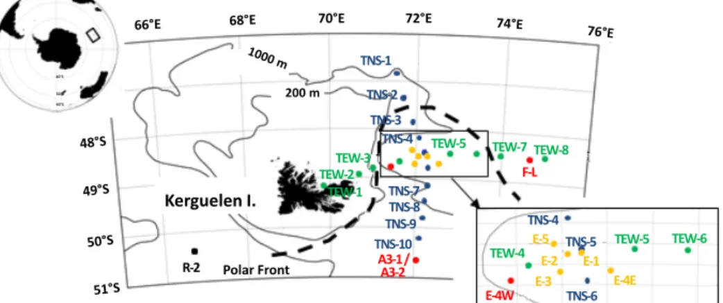
be-Kerguelen I. Polar Front R-2 A3-1 / TNS-10 TNS-9 TEW-7 TEW-8 TEW-2 TEW-6 TEW-5 TEW-5 TEW-4
E-4W E-3 E-4E
E-1 E-2 E-5 TNS-6 TNS-4 TNS-8 TNS-4 TEW-3 TEW-1 TNS-5 TNS-7 F-L A3-2
Figure 1. Map of the KEOPS2 study area and station locations. The locations of the stations are marked by coloured dots. The southern station A3 (red dot) was visited twice at the beginning (station A3-1) and the end (station A3-2) of the KEOPS2 survey. This station, A3, situated in the middle of the shelf, was the reference station for the shelf bloom observed during KEOP1. The stations of the north–south transect (shown by blue dots) are located in oceanic waters and were sampled just after the first visit to A3, from south to north (stations TNS1 to TNS10), from the central plateau (TNS10) across the recirculation feature (TNS7 toTNS3) and the Polar Front (TNS3, TNS2) and into subantarctic waters (TNS1). Station R-2 (black dot) in the west of the Kerguelen Plateau represented a HNLC reference station. The TEW transect (east–west transect) was sampled from west to east from the near coast of Kerguelen Island (TEW1) above the shelf (TEW32) and shelf break (TEW3) across the middle of the recirculation system (TEW4 to TEW6), and beyond the southward meandering Polar Front (TEW7 and TEW8) in the extreme east of the study region. The survey ended with a quasi-Lagrangian time series (stations E1–E5 in orange dots in the zoom panel), during a progressive phase of the bloom within the recirculation system in the meander of the Polar Front. In addition, one station (station F-L) situated in high-biomass waters in the extreme north-east of the study region, near the downstream location of the PF, was sampled within the period of the time series.
tween TEW3 and TEW4 where the southern branch of the PF flows northwards along the shelf break, and secondly be-tween TEW6 and TEW7, where the PF is directed south-wards after a semicircle trajectory maintaining a large sta-tionary meander in this area. The most westerly stations were located over the inner (TEW1) and outer (TEW2) parts of the Kerguelen shelf. The most easterly stations (TEW7 and TEW8) were situated in Subantarctic Mode Water whereas the central section (TEW4 to TEW6) within the station-ary meander was covered by mixed Antarctic surface water (Farías et al., 2015; Trull et al., 2015).
In addition, intensive sampling (24 h) was performed at nine strategic stations (Fig. 1) located in the eastern bloom in the Polar Front zone (F-L station), in the north-eastern bloom (set of E stations), in the south-eastern bloom above the Ker-guelen Plateau (A3 station) and in the deep waters south-west of the Kerguelen Islands considered as a HNLC refer-ence station (R station). Station A3 (common with KEOPS1) was sampled twice during KEOPS2: at the winter (A3-1) stage and the spring stage (A3-2). The patterns of change over time of the north-eastern bloom, located in a complex recirculation area inside the stationary meander of the Polar Front (Park et al., 2014; Zhou et al., 2014), was studied by a quasi-Lagrangian survey including five stations (E1-E2-E3-E4E-E5).
Real-time-satellite images (chlorophyll and altimetry) in combination with trajectories of 50 drifters released during the first part of the cruise were used to carefully decide the
positions of these five stations (Trull et al., 2015, their Fig. 2). In addition, we visited a productive station (E4W, red dot in Fig. 1) located in the plume of chlorophyll observed down-stream of the plateau and close to the jet induced by the PF.
2.2 Mesozooplankton sampling
Zooplankton collection was conducted at 27 stations with a double Bongo (60 cm mouth diameter) with one 330 µm mesh net and a 120 µm mesh net mounted with filtering cod ends. Hauls were done from a 250 m depth to the surface at 0.5 ms−1. The stations of the TNS transect (stations TNS 1 to TNS10) and the stations of the TEW transect (stations TEW1 to TEW8) were each sampled once. During the intensive sta-tions study (including A3 – which was visited twice – R2, F-L, and the set of E stations), zooplankton samples were taken twice daily, by day and by night (stations were named R2-d and R2-n, for instance).
For each sampling station, two successive net hauls at each station were done: the first net haul was taken for ZOOSCAN processing, taxonomy study and dry weight measurements, and a second net haul was taken for isotope analysis. The cod-end contents of the first haul were kept fresh and split into two parts with a Motoda box (Motoda, 1959). The first part was preserved in 4 % borax-buffered formalin sea-water for further laboratory study of zooplankton commu-nity structure (taxonomy, abundance and size structure) and for biomass estimates from organism biovolume (see
be-low). The second half of the sample was preserved for dry weight measurements. As many of the 120 µm size nets were clogged with phytoplankton cells and aggregates, we could not finally use the sample for dry weight measurements and ZOOSCAN processing. However we used the 120 µm mesh net samples for isotope analysis (as described in the follow-ing paragraph).
To prepare samples for isotope analysis, size fractions were obtained as follows. Samples from the second 330 µm net haul at each station were passed sequentially through five sieves arranged in a column (2000, 1000, 500, 200 and 80 µm meshes). The three largest sizes were then collected, and for the largest size (2000 µm) large organisms such as salps and euphausiids were separated into additional con-tainers. To provide more material for the two smallest sizes (200, 80 µm), these materials were retained on the sieves and the contents of the 120 µm net haul were passed through the entire set of five sieves (with the overlying 2000, 1000 and 500 µm sieves serving to block larger organisms and aggre-gates, but without those materials being collected). All sam-ples were placed in small containers and immediately deep-frozen (−80◦C).
2.3 Abundance and biomass using the Zooscan
For each station, the cod-end content of a 330 µm mesh size net was processed using ZOOSCAN (www.zooscan. com) to determine the zooplankton community size struc-ture. ZOOSCAN has recently been used to study the zoo-plankton community in various areas and has been validated by comparisons with traditional sampling methods (Gros-jean et al., 2004; Schultes and Lopes, 2009; Gorsky et al., 2010). Our ZOOSCAN setup is similar to the one described by Gorsky et al. (2010), and our sample processing protocol is fully presented in Nowaczyk et al. (2011), following the recommendations of Gorsky et al. (2010).
After homogenization, each sample was quantitatively split with a Motoda box once back in the laboratory and a fraction of each preserved sample containing a minimum of 1000 particles (in general 1/32 or 1/64 of the whole sam-ple) was placed on the glass plate of the ZOOSCAN. Or-ganisms were carefully separated one by one manually with a long wooden needle, in order to avoid overlapping. Each image was then run through the ZooProcess plug-in using the image analysis software Image J (Grosjean et al., 2004; Gorsky et al., 2010). Several measurements of each organ-ism were then computerized. Organorgan-ism size is given by its equivalent circular diameter (ECD) and can then be con-verted into biovolume, assuming each organism is an ellip-soid (more details in Grosjean et al., 2004). The lowest ECD detectable by this scanning device is 300 µm. To discriminate between aggregates and organisms, we used a training set of about 1000 objects which were selected automatically from 40 different scans. This protocol allows discrimination be-tween aggregates and organisms by building the initial
train-ing set of images. The biovolume (BV; mm3)was calculated from the organism image areas and morphometric parame-ters. In order to estimate the biomass of each organism, we used the same conversion as in Carlotti et al. (2008); each measured biovolume (BV; mm3)of a zooplankton individual was converted into biomass (W , in units of mg dry weight, DW) using the following relationship: log (W ) = 0.865 log (BV) − 0.887 (Riandey et al., 2005). Carbon content was as-sumed to be 50 % of body dry weight.
In this article, the terms “ZOOSCAN abundance” and “ZOOSCAN biomass” will designate the values derived from the laboratory ZOOSCAN processing. The abundance and biomass of organisms were then grouped into four size fractions (< 500, 500–1000, 1000–2000 and > 2000 µm) based on their ECD, and summed to deliver the total abun-dance and biomass per sample over the upper 250 m.
The choice of the net haul sampling depth was based on mixed layer depth found at the first station of the cruise, and maintained afterwards. Abundance and biomass values are normalized to the volume of water filtered in situ. An ANOVA test (5 % significance level) was used to test differ-ences of abundance and biomass between stations or oceanic areas.
2.4 Taxonomic determination
Common taxa were counted with the binocular microscope for taxonomy. For the 330 µm mesh size net, around 600 organisms were counted from subsamples 1/32 or 1/64). For the 120 µm mesh size net, around 400 organisms were counted from diluted samples (dilution from one to ten thou-sandths). The whole sample was examined for either rare species and/or large organisms (i.e. euphausiids, amphipods). Identification of the copepod community was done down to species level and groups of developmental stage when possible. Species/genus identification was done according to Rose (1933), Tregouboff and Rose (1957) and Razouls et al. (2014). Organisms other than copepods as well as mero-plankton were identified down to taxa levels. Identifications were done to genus level for copepods, amphipods, pelagic molluscs, polychaetes, Thaliacea and Cnidarians; and to taxa level for other major holoplanktonic and meroplanktonic groups. To identify which taxonomic groups contribute to the four size fractions defined from ZOOSCAN measurements done on the 330 µm mesh net samples (see above), each observed organism was classified as small, medium, large or very large mesozooplankton, which approximately corre-sponds to the four size fractions determined by ZOOSCAN (see above). Similarly, the organisms observed and counted from the 120 µm mesh size net samples were also classified into small and medium size fractions. Distribution in larger size fractions was not considered from the 120 µm mesh size net samples, the large organisms being undersampled.
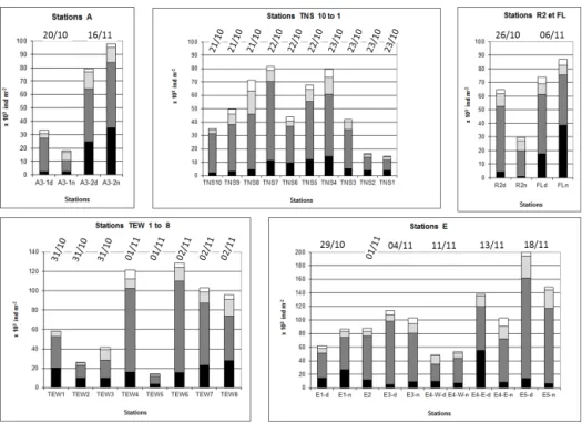
Figure 2. Integrated 0–200 m mesozooplankton abundance counted from ZOOSCAN for the different stations sampled during KEOPS2 with size-fraction distributions. Size fractions: < 500 µm, black; 500–1000 µm, dark grey; 1000–2000 µm, light grey; > 2000 µm, white.
2.5 Biomass measurement
The subsample of the 330 µm mesh net for bulk biomass measurement was filtered onto a weighed and pre-combusted GF/F filter (47 mm) which was quickly rinsed with distilled water and dried in an oven at 60◦C for 3 days on board. The dry weight (mg) of 19 samples was calcu-lated from the difference between the final weight and the weight of the filter, and biomass (mg DW m−2)was extrapo-lated from the total volume sampled by the net.
2.6 Stable isotope analysis
Before processing, identification of the broad taxonomic composition of each sample preserved for isotopic mea-surements was performed under a binocular microscope. When possible, the main group of organisms in the largest > 2000 µm size fraction were sorted out and processed sep-arately. Then, zooplankton fractions were freeze-dried and ground into a homogeneous powder. As they may con-tain carbonates, an acidification step was necessary to re-move 13C-enriched carbonates (DeNiro and Epstein, 1978; Søreide et al., 2006). A subsample was acidified with 1 % HCl, rinsed, dried and used for determination of δ13C val-ues, while the other untreated subsample was used for deter-mination of nitrogen isotopic composition. Three replicates were performed on each plankton fraction per sampled sta-tion for both δ13C and δ15N values. Stable isotope measure-ments were performed with a continuous-flow isotope-ratio mass spectrometer (Delta V Advantage, Thermo Scientific,
Bremen, Germany) coupled to an elemental analyzer (Flash EA1112 Thermo Scientific, Milan, Italy). Results are ex-pressed in parts per thousand (‰) relative to Vienna Pee Dee Belemnite and atmospheric N2 for δ13C and δ15N, respec-tively, according to the equation: δX = [(Rsample/Rstandard)− 1] ×103, where X is 13C or 15N, and R is the isotope ra-tio13C /12C or15N /14N, respectively. Calibration was per-formed using certified reference materials (USGS-24, IAEA-CH6, -600 for carbon; IAEA-N2, -NO-3, -600 for nitro-gen). Analytical precision based on repeated analyses of ac-etanilide (Thermo Scientific) used as an internal standard was < 0.15 ‰. Percentage of organic C and organic N were ob-tained using the elemental analyzer and were used to calcu-late sample C / N ratios.
Lipids are depleted in δ13C relative to proteins and carbo-hydrates, and variation in lipid content between organisms can introduce considerable bias into carbon-stable isotope analyses (Bodin et al., 2007; Post et al., 2007). Like most po-lar marine organisms (Lee et al., 2006), KEOPS2 zooplank-ton fractions could present a high lipid content (up to 20 % dry mass, data not shown), reflected by high C / N values. Thus, δ13C acidified sample values of fractions > 200 µm were corrected according to the formula calculated by Post et al. (2007) for aquatic organisms, using the C / N ratio of each sample: δ13Cnormalized=δ13Cacidified– 3.32 + 0.99 × C / N
Acidified δ13C values of the lowest size fraction (80– 200 µm) were not lipid-corrected due to their low lipid con-tent (< 5 %, data not shown). The resulting δ13Cnormalized provides an estimate of δ13C corrected for the effects of
lipid concentration. Lipid correction calculated by Smyntek et al. (2007) for zooplankton give δ13C values 0.63 ± 0.01 ‰ lower than those of Post et al. (2007). As δ13C values pro-vided by Trull et al. (2015) were not lipid-normalized, acid-ified δ13C values for all zooplankton size fractions are indi-cated in Table 2, along with lipid-normalized δ13C values, to allow comparisons between the two data sets.
To consider the relationships between zooplankton and phytoplankton, we used the groups of stations (T-groups) de-fined by Trull et al. (2015) based on chemometric measure-ments of phytoplankton. The HNLC reference station R2 be-longed to T-group 1, along with station TEW4. Stations lo-cated on the plateau (A3 and E4) and in the eddy (E1 to E5) are included in T-group 2 and T-group 3, respectively. The two most easterly stations, located in the open ocean near the Polar Front (F-L and TEW8), belonged to T-group 5. Trull’s T-group 4 corresponded to coastal stations not sampled for zooplankton analysis.
2.7 Data analysis
The effect of stations and dates (n = 12) on zooplankton abundance and biomass was tested statistically using one-way ANOVA with the statistical software Statistica v7. The statistical significance was tested at the 95 % confidence level. Community patterns for taxa abundance were explored using the Primer (V6) software package which has been shown to reveal patterns in zooplankton communities (e.g. Clarke and Warwick, 2001; Wishner et al., 2008). Data sets were power-transformed (fourth root), and the Bray–Curtis dissimilarity index between stations (Bray and Curtis, 1957) was calculated employing all taxonomic categories that con-tributed at least 1 % to any sample in that data set. Dif-ferent groups of zooplankton (BC groups) were individual-ized based on their taxonomic composition. Mean C- and N-stable isotope values among size fractions and between day and night within each fraction were compared by one-way ANOVAs followed by Tukey post-hoc tests, after testing for normality by a Levene test.
3 Results
3.1 Hydrology and trophic conditions
The KEOPS2 campaign was characterized by conditions of complex circulation and rapidly changing phytoplank-ton biomass (see Trull et al., 2015, their Figs. 1 and 2 and Suppl.). During the survey, the horizontal circulation pattern was dominated by the northernmost branch of the PF (Park et al., 2014) flowing across the plateau in the narrow, mid-depth (1000 m) channel just to the south of Kerguelen Island (Fig. 1). After passing to the east of the plateau, the jet flows outside the shelfbreak northwards and enters in a bathymet-rically trapped cyclonic recirculation system (d’Ovidio et al., 2015; Park et al., 2014, Trull et al., 2015). The variations of
the PF position during the KEOPS2 survey are documented in Trull et al. (2015, in supplement). The PF jet separated the central plateau and offshore stations to the south (A3, TNS 10 to TNS 3, TEW3 to TEW6, and E stations) from those to the north and east (TNS1,TNS2, TEW7, TEW8, F-L) and those stations close to the coast (TEW1 and TEW2).
At the beginning of our study (during the visit to station A3-1 and to the TNS transect), slight chlorophyll accumula-tion was visible from satellite images (see complementary information on satellite-image-derived primary production supplied by Trull et al. (2015), their Fig. 2 and Supplement), but the sampling on the first visit to station A3 (A3-1, on 20 October) revealed pre-bloom conditions on the plateau and some stations (TNS9, TNS4) of oceanic waters (Jouan-det et al., 2014; Lasbleiz et al., 2014). The bloom started in earnest in early November, first massively on the plateau and in coastal waters, and secondly in spatially heterogeneous low biomass oceanic waters (during our TEW transect and stations E1-E3), with higher chlorophyll values at stations (TEW 7, TEW 8, F-L) downstream from the Polar-Front bloom (Lasbleisz et al., 2014; Trull et al., 2015). In mid-November, the central plateau bloom was well-developed (station A3-2) and afterwards started to decrease slightly, whereas downstream in the Polar Front, bloom was most ex-tensive south of PF and showed its highest biomass there (sta-tions E4–5).
The vertical depth stratification was variable over both space and time (see Trull et al. (2015), their Table 4a). Station R2 presented a MLD around 117 m. At station A3, the wa-ter column was characwa-terized by a deep mixed layer (around 150 m) during the pre-bloom (station A3-1) and early bloom (station A3-2) surveys, with a range of 120 to 171 m (Jouan-det et al., 2014). The Chl a concentrations showed a fourfold increase from A3-1 (21 October) to A3-2 (15–17 Novem-ber), with Chl a concentrations at the surface increasing from 0.5 to 2 mg m−3 (Jouandet et al., 2014, their Figs. 1 and 2). The mixed layer depth of the TNS stations south of the PF decreased northward from around 150 m (TNS10) to 100 m (except TNS6), with accompanying chlorophyll a concentrations between 0.5 and 1.5 mg m−3 (Lasbleisz et al., 2014, their Fig. 3). During the following visits to the region within the recirculation system in the PF meander (square zoom in Fig. 1), the MLD progressively decreased from 100 to 50 m (stations E1, TEW4 to TEW5), and then below 50 m (stations TEW6, E2 to E5, – except E4 decreas-ing slightly around 70 m) with similar chlorophyll a concen-trations between 1.0 and 1.5 mg m−3(Lasbleisz et al., 2014, their Fig. 4). The highest chlorophyll a concentrations (val-ues up to 4.7 mg m−3)were found in the 40 upper metres of the 100 m water column of the coastal stations (TEW1 and TEW2, Lasbleisz et al., 2014), whereas the TEW3 above the shelf break presented lower chlorophyll a concentrations (< 1.0 mg m−3)in its 60 m mixed layer, possibly due to its proximity to the PF jet.
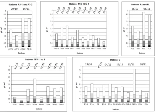
Figure 3. Integrated 0–200 m mesozooplankton biomass estimated from ZOOSCAN for the different stations sampled during KEOPS2 with size-fraction distributions. Size fractions: < 500 µm, black; 500–1000 µm, dark grey; 1000–2000 µm, light grey; > 2000 µm, white.
Abundances 0 50 100 150 200 250
18-Oct 23-Oct 28-Oct 02-Nov 07-Nov 12-Nov 17-Nov 22-Nov TNS TEW E A3 R F x 10 3 In d m -2 A F-L 18/10 23/10 28/10 02/11 07/11 12/11 17/11 22/11 g C m -2 Biomasses 0 1 2 3 4 5 6
18-Oct 23-Oct 28-Oct 02-Nov 07-Nov 12-Nov 17-Nov 22-Nov TNS TEW E A3 R F B F-L 18/10 23/10 28/10 02/11 07/11 12/11 17/11 22/11
Ratio Abundance / Biomass
0 20 40 60 80 100 120 140 160 180
18-Oct 23-Oct 28-Oct 02-Nov 07-Nov 12-Nov 17-Nov 22-Nov TNS TEW E A3 R F C F-L x 10 3 In d g C -1 18/10 23/10 28/10 02/11 07/11 12/11 17/11 22/11
Time (day / month) Time (day / month)
Time (day / month)
Figure 4. (a) Abundance and (b) biomass values and (c) ratio abun-dance on biomass for the different stations visited during KEOPS2 over sampling dates. Abundance and biomass values from Figs. 2 and 3.
The sampled stations in the Subantarctic Mode Water presented very low chlorophyll a concentration in TNS2 (0.65 mg m−3 in the upper 60 m), but much higher 10 days later, in TEW-7 and TEW-8 (average above 3 mg m−3in the upper 60 m, with peak concentrations up to 5.0 mg m−3; Las-bleisz et al., 2014, their Fig. 4).
3.2 Temporal and spatial variations of zooplankton
abundance and biomass
Zooplankton abundances and biomass from ZOOSCAN pro-cessed samples of the 330 µm mesh net varied from 14 × 103 to 200 × 103ind m−2(Fig. 2) and from 0.25 to 4.94 g C m−2 (Fig. 3), respectively. Comparisons of abundance (ind m−2) and biomass (g C m−2) between ZOOSCAN-derived data and direct measurements showed that ZOOSCAN-derived data slightly overestimated direct measurements from regres-sion forced through the origin: slope equal to 1.0015 for abundance (R2=0.75, n = 37, p < 0.01) and slope equal to 1.1246 for dry weight (R2=0.803, n = 19, p < 0.01).
Abundance values followed a normal distribution pattern with an average of 73103ind m−2 (SD: 42). ANOVA with main effects (stations and dates) without interaction showed clear effects for dates (p < 0.05) but not for stations. All abundance values plotted against dates (Fig. 4a) showed a general increase, and the linear regression (R2=0.42, n = 37) predicted a ratio of 3.7 between abundance at the begin-ning and at the end of the survey. Highest abundance (above the regression line on Fig. 4a) was observed for oceanic sta-tions within the PF meander, both for the stasta-tions of the two transects (stations TNS4, 5, 7, 8, and TEW 4, 6, 7, 8, and stations E, except for E4-West). By contrast, the low-est abundance was found to the east and north of this PF meander, as well as for the first visit to A3. One exception was station TEW5, which presented the lowest abundance, whereas nearby spatial and temporal sampling stations pre-sented much higher abundance. Between the two visits to
sta-tion A3 at the beginning and the end of the survey, the total abundance had multiplied by 3.5.
The fraction 500–1000 µm (see Fig. 3) presented the most abundant number of organisms (62.0 % on average), followed by the < 500 µm fraction (18.8 % on average), the 1000–2000 µm fraction (14.2 % on average) and the > 2000 µm fraction (5.0 % on average). The contribution of the smaller size fraction (< 500 µm) increased with time from the beginning to the end of the survey (8.1 % on av-erage), whereas the 500–1000, 1000–2000, and > 2000 µm decreased to 5.0, 0.8 and 2.3 %, respectively. However, these temporal changes were not significant in any of the four re-gressions due to the variability in size distribution between the stations. In addition, no clear diurnal pattern was ob-served from the day/night samplings performed at nine sam-pling dates.
Log-transformed biomass values followed a normal dis-tribution pattern. As for the abundance, ANOVA with main effects (stations and dates) without interaction for biomass values showed an effect for dates (p < 0.05) but not for sta-tions. Average biomass was 2.32 g C m−2 (SD: 1.33), and the linear regression against time (not significant) predicted a ratio of 1.7 between biomass values at the beginning and the end of the survey (Fig. 4b). However, the biomass ratio between the two visits at station A3 showed an increase of 2.9, whereas the biomass values at station E (the Lagrangian survey) showed a slightly decreasing trend (with the excep-tion of E4-En). The fracexcep-tion > 2000 µm represented the high-est biomass of organisms (57.1 % on average), followed by the 1000–2000, 500–1000 and < 500 µm fractions with 22.8, 18.2 and 1.9 % on average, respectively (see Fig. 2). None of the regressions between the percentage value and dates presented a significant correlation, and the slopes of the re-gression were all near to zero for the intermediate size frac-tions. From the beginning to the end of the survey, the largest size fraction (> 2000 µm) decreased in its contribution to the biomass (−1.5 %), whereas the contribution to the biomass increased with time by 0.1, 0.5 and 0.9 %, respectively, for the 1000–2000, 500–1000 and < 500 µm fractions.
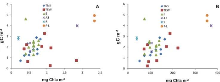
The total zooplankton biomass values presented a signifi-cant correlation (p < 0.01) with the average chlorophyll con-centrations in the 100 upper metres, as well as with the in-tegrated chlorophyll concentrations in the mixed layer depth (Fig. 5). Only stations TEW1 and TEW2 presented low zoo-plankton biomass for relatively high fluorescence concen-trations (> 1 µg Chl a L−1, Fig. 5a), but not versus the inte-grated Chl a biomass in their shallow (< 80 m) mixed layers (Fig. 5b).
3.3 Metazooplankton community composition and
distribution
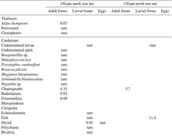
From the 330 µm mesh size net, 65 taxa were identified for the 37 stations of this study (Table 1) with 26 genera/species of copepods. Copepods contributed the bulk of the
zooplank-0 1 2 3 4 5 6 0 0.5 1 1.5 2 2.5 TNS TEW E A3 R F gC m -2 mg Chla m-3 A F-L gC m -2 mg Chla m-2 B 0 1 2 3 4 5 6 0 100 200 300 400 TNS TEW E A3 R FF-L
Figure 5. Zooplankton biomass values against average Chl a in the upper 100 m (a) and against the integrated Chl a in the mixed layer depth (b) for the different stations visited during KEOPS2. Biomass values from Fig. 3.
ton community abundance with 78.4 % (SD = 13.13 %) of the counted organisms over the whole area, and copepodites represented a little more than half of the counted cope-pods (mean = 52.5 %, SD = 8.2 %). ANOVA with main fects (stations and dates) without interaction showed no ef-fect either for dates or for stations, either for the percentage of copepods against the whole zooplankton abundance, or for the percentage of copepodites stages against the total cope-pods abundance. Nauplii represented an average 2 % of the total abundance, and showed an increasing abundance with time up to 4 %, although they were undersampled with our net. The copepod communities were dominated by
Cteno-calanus citer, followed by Oithona similis and O. frigida, Metridia lucens, Scolecithricella minor, Calanus simillimus, Paraeuchaeta spp., Rhincalanus gigas, and near the coastal
area Drepanopus pectinatus. Other dominant taxa were the different larval stages of euphausiids (eggs, nauplii, metanau-plii, proto et metaozoe), appendicularians (Oïkopleura spp.,
Fritillaria spp.), chaetognaths, pteropods (Limacina retro-versa) and amphipods (Themisto gaudicaudii, Hyperia spp.).
Radiolarians and foraminifera were regularly sampled as well. In some stations, other taxa occurred in low numbers, such as salps.
With the 120 µm mesh size net, the number of identi-fied taxa for the 37 stations was reduced to 28 taxa (Ta-ble 1), strongly dominated by copepod species. Copepod larval forms as nauplii, undetermined copepod nauplii and copepodites, and copepodid stages of Oithona sp., Oncoea sp., and Ctenocalanus citer represented 20.4 % of organisms in 120 µm mesh size nets. Adult forms (73 % of the organ-isms in nets) were mainly from small and medium size cope-pods such as Oithona similis and O. frigida, Microsetella
rosea, Oncaea spp., Triconia sp., Microcalanus pygmaeus
and Scolecithricella minor. Other dominant taxa in this net were the different larval stages of euphausiids, appendicular-ians, chaetognaths, pteropods (Limacina antarctica), as well as, at a few stations, echinoderm larvae.
Comparison between the community compositions in the two nets clearly showed that some key groups were under-sampled in the 330 µm mesh net: mainly the larval stages of many copepods, small copepods such as Oithona sp.
Mi-Copepods Oithona similis 8.1 2.8 489.8 1362.5 Oithona frigida 14.8 2.8 71.5 1362.5 Microsetella rosea 1.9 79.0 Oncaea spp. 1.3 0.1 58.2 53.6 Triconia sp. 8.7 20.7 11.4 Clausocalanus laticeps 3.9 0.8 1.5 0.1 Ctenocalanus citer 35.8 56.5 47.8 195.7 Microcalanus pygmaeus 0.7 23.2 Metridia lucens 9.6 8.9 4.6 39.3 Calanus propinquus 0.02 Calanus simillimus 6.45 1.9 1.4 1.62 Calanoides acutus 1.1 1.6 0.2 0.41 Scolecithricella minor 9.2 6.4 10.1 8.4 Scaphocalanus spp. 0.7 2.5 Drepanopus pectinatus 0.6 2.7 1.4 13.7 Pleuromamma robusta 0.9 0.2 0.4
Candacia maxima rare rare
Heterorhabdus spp. rare rare
Aetideus armatus rare rare
Haloptilus oxycephalus rare rare
Paraeuchaeta spp. 0.54 14.29 14.1
Rhincalanus gigas 2.93 7.34 3.1 1.1 7.9 26.63
Subeucalanus longiceps 0.14 0.02 0.4
Euchirella rostramagna rare 0.04 0.04
Gaetanus pungens rare
Undeuchaeta incisa rare
Undetermined nauplii 2.1 1071.7
Undetermined copepodites 22.4 253.5
330 µm mesh size net 120 µm mesh size net
Adult forms Larval forms Eggs Adult forms Larval forms Eggs
Euphausiids Undetermined species 0.27 6.22 32.23 6.8 33.2 Ostracods 2.3 7.9 Isopods 0.05 Mysid rare Decapod rare Amphipods Themisto gaudicaudii 0.26 Hyperia spp. 0.86 Primno macropa 0.10 Vibilia sp. rare 0.04 Scina sp. rare Molluscs Limacina retroversa 3.45 33.2
Limacina helicina rare
Spongiobranchaea sp. rare Clio sp. rare Polychaetes Pelagobia sp. 0.22 Tomopteris spp. rare Travisiopsis sp. rare
Undetermined rare 0.32 rare 9.28
Table 1. Continued.
330 µm mesh size net 120 µm mesh size net
Adult forms Larval forms Eggs Adult forms Larval forms Eggs
Thaliacea
Salpa thompsoni 0.07
Pyrosomid rare
Ctenophores rare
Cnidarians
Undetermined larvae rare rare
Undetermined adult rare
Bougainvillia sp. rare
Dimophyes arctica rare
Pyrostephos vanhoeffeni rare
Rosacea plicata rare
Muggiaea bargmannae rare
Solmundella bitentaculata rare
Pegantha sp. rare Chaetognaths 4.15 5.7 Radiolarians 0.93 Foraminifera 0.98 Meroplankton Cirripedia Echinodermata rare Fish rare 11.4 Mysid 0.05 rare Polychaeta rare Bivalvia rare
crosetella rosea, Oncaea spp. Triconia sp., Microcalanus pygmaeus, Ctenocalanus citer. The impact of 120 µm mesh
size and clogging on the larger planktonic organisms was dif-ficult to assess as many groups were in any case in low den-sity in the 330 µm mesh size net, except for the copepods
Clausocalanus laticeps, Calanus simillimus and Calanoides acutus.
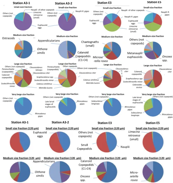
The taxonomic distributions are presented in more detail for stations A3 (the two visits A3-1 and A3-2) and for sta-tions E3 and E5 in Fig. 6 for the four size fracsta-tions from the 330 µm mesh size net sample, and only in the small and medium size fractions from the 120 µm mesh size net sample. The distribution pattern from the 330 µm mesh size net samples is first presented below. The zooplankton commu-nity structure in A3-1 was numerically dominated by the medium size fraction (nearly comparable to the fraction 500–1000 µm in total abundance in Fig. 2) comprising more than 50 % of copepods, characterized by the abundant cy-clopoïd Oithona similis, along with unspecified calanoid copepodites, and the harpacticoid Microsetella rosea. The rest of this fraction included metanauplii of euphausiids, ap-pendicularians, ostracods and small chaetognaths. The frac-tion of “large size” mesozooplankton, similar to the 1000– 2000 µm fraction counted with ZOOSCAN and representing 10.7 % of the total abundance, was composed of 98 %
cope-pods with some major taxa (Ctenocalanus citer, Metridia
lucens, Scolecithricella minor, Calanus simillimus, Scapho-calanus spp., ClausoScapho-calanus laticeps), and early copepodites
of Paraeuchaeta and of Calanidae. The highest size fraction was dominated by more than 75 % by Rhincalanus gigas and amphipods Hyperia spp. and Themisto gaudicaudii. It corre-sponds to the fraction > 2000 µm from the ZOOSCAN which contributes to two-thirds of the mesozooplancton biomass at station A3-1 (see Fig. 2). The lowest size fraction was mainly composed of euphausiid eggs and nauplii, copepod nauplii, small forms of the pteropod Limacina retroversa and in small densities foraminifera and radiolarians. As a whole, the mesozooplancton community in A3-1 was mainly com-posed of herbivorous species in all fractions, such as the copepods R. gigas, C citer, O. similis, M. rosea, but also pteropod L. retroversa, appendicularians and different nau-plii stages of copepods and euphausiids. In lowest densities, omnivores and detritivores (such as the copepods M. lucens,
S. minor, C. simillimus) and carnivores (such as chaetognaths
and amphipods, and the copepod Paraeuchaeta) were found. During the second visit to station A3 (A3-2), the size dis-tribution in abundance was dominated by fractions with ECD < 1000 µm (up to 83 % of the total abundance, see in Fig. 3). The taxa distribution in A3-2 differed from the first visit (sta-tion A3-1) both in the “small” size frac(sta-tions by an increase in
Figure 6. Distributions of main taxa abundance at stations A3-1, A3-2, E3 and E5 from binocular observation. Distributions are presented from left to right for the four stations, and from top to bottom for the four size fractions (four upper bands: small, medium, large, and very large) observed in the 330 µm mesh size net samples, and for the two lower size fractions (two lower upper bands: small and medium) for the 120 µm mesh size net samples. Distributions are average values between day and night samples. For each size fraction (the four pie charts on the same horizontal band), the colour labels for the different taxa are similar.
copepod nauplii and euphausiid eggs, and in the “medium” size fraction by a large proportion of appendicularians and early copepodid stages of copepods. The two largest frac-tions (“large” and “very large”) were not very different at A3-1 and A3-2 in taxonomic composition and distribution (the only difference being the appearance of late larval stages of euphausiid in the “very large” fraction).
The major features in taxonomic changes between sta-tions E3 (04 November) and E5 (18 November) (Fig. 6) were the increasing contribution of calanoid copepodids in the medium and large size fractions, with the concomitant increase of contribution of these fractions to the total abun-dance (see also Fig. 2), and the increase of euphausiid larvae in the largest fraction. The smaller fraction presented a rather stable distribution of dominant taxa, with copepod nauplii
and Limacina as dominant groups (Fig. 6). As a whole, while omnivores, carnivores and scavengers are present, the herbiv-orous component is strongly dominant with all these larval forms. It is of interest to note that the dominant species for the different fractions at E5 were quite similar to those at A3-1, but with the noticeable difference that many larval stages occurred in all size fractions, inducing the highest observed abundance during the survey (see Fig. 2), although finally representing a lower biomass (see Fig. 3).
In the 120 µm mesh size net samples, the taxonomic ob-servation generally delivered the same dominant taxa in the medium size fraction as for the 330 µm mesh size net, but with larger proportions of small copepodid forms and small adult copepods, such as Oncoea spp. and Microsetella rosea.
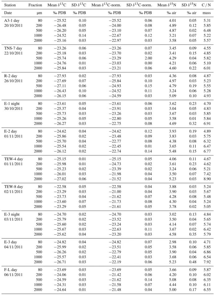
Table 2. Isotopic composition of size-fractionated zooplankton (mean and standard deviation). Mean δ13C, values of acidified samples; mean δ13C-norm, lipid-normalized values (except for the lowest size fraction); mean δ15N, values of untreated samples.
Station Fraction Mean δ13C SD δ13C Mean δ13C-norm. SD δ13C-norm. Mean δ15N SD δ15N C / N
Date µm ‰ PDB ‰ PDB ‰ PDB ‰ PDB ‰ air ‰ air mass
A3-1 day 80 −25.52 0.10 −25.52 0.06 4.01 0.05 5.31 20/10/2011 200 −26.48 0.05 −24.00 0.08 4.89 0.12 5.85 500 −26.20 0.05 −23.10 0.07 4.87 0.02 6.48 1000 −24.52 0.14 −22.67 0.12 3.21 0.07 5.22 2000 −25.16 0.03 −22.97 0.03 3.58 0.05 5.57 TNS-7 day 80 −23.26 0.06 −23.26 0.07 3.45 0.09 4.55 22/10/2011 200 −25.18 0.03 −23.70 0.02 3.41 0.15 4.85 500 −25.74 0.06 −23.29 2.00 4.29 0.04 5.82 1000 −24.76 0.01 −23.03 0.00 4.21 0.06 5.10 2000 −25.84 0.03 −23.21 0.06 4.60 0.22 6.01 R-2 day 80 −27.93 0.02 −27.93 0.03 4.36 0.08 4.87 26/10/2011 200 −27.69 0.07 −25.84 0.10 4.97 0.03 5.23 500 −27.11 0.06 −24.93 0.15 4.79 0.19 5.55 1000 −26.43 0.10 −24.52 0.11 3.24 0.06 5.28 2000 −26.15 0.06 −24.59 0.03 5.09 0.10 4.93 E-1 night 80 −23.61 0.05 −23.61 0.06 3.62 0.23 4.70 30/10/2011 200 −25.37 0.04 −23.91 0.03 3.04 0.05 4.83 500 −25.73 0.03 −23.26 0.03 3.67 0.03 5.85 1000 −25.26 0.05 −22.80 0.05 3.58 0.01 5.84 2000 −26.27 0.03 −22.75 0.08 4.69 0.32 6.91 E-2 day 80 −24.62 0.04 −24.62 0.12 3.93 0.19 4.89 01/11/2011 200 −25.86 0.02 −23.48 0.09 3.83 0.03 5.75 500 −25.70 0.04 −22.77 0.08 4.38 0.08 6.32 1000 −25.54 0.02 −22.45 0.01 3.65 0.11 6.47 2000 −26.12 0.02 −22.74 0.14 5.48 0.15 6.77 TEW-4 day 80 −25.15 0.01 −25.15 0.05 4.06 0.11 4.67 01/11/2011 200 −25.98 0.01 −24.73 0.02 3.61 0.23 4.62 500 −25.23 0.02 −23.39 0.02 3.24 0.06 5.21 1000 −26.01 0.03 −21.98 0.04 3.50 0.07 7.42 2000 −27.02 0.06 −21.52 0.04 5.23 0.03 8.90 TEW-8 day 80 −22.58 0.05 −22.58 0.04 3.88 0.03 5.24 02/11/2011 200 −23.29 0.03 −21.00 0.04 3.90 0.03 5.67 500 −23.73 0.04 −21.62 0.07 4.28 0.08 5.48 1000 −23.60 0.07 −21.73 0.08 4.30 0.04 5.24 2000 −23.29 0.05 −21.61 0.05 3.78 0.02 5.05 E-3 night 80 −24.70 0.02 −24.70 0.03 3.02 0.13 4.84 03/11/2011 200 −25.79 0.02 −23.52 0.03 3.50 0.04 5.65 500 −25.60 0.02 −23.24 0.03 4.14 0.07 5.74 1000 −25.67 0.03 −22.63 0.11 3.67 0.02 6.42 2000 −25.62 0.04 −23.20 0.03 4.58 0.35 5.79 E-3 day 80 −24.82 0.04 −24.82 0.07 2.98 0.10 4.71 04/11/2011 200 −25.99 0.02 −23.51 0.05 3.58 0.06 5.85 500 −26.26 0.02 −22.79 0.05 3.90 0.04 6.86 1000 −25.57 0.03 −22.41 0.03 3.68 0.06 6.54 2000 −26.71 0.03 −22.19 0.06 5.23 0.48 7.92 F-L day 80 −23.69 0.03 −23.69 0.05 3.66 0.09 5.87 06/11/2011 200 −24.06 0.01 −21.42 0.06 4.20 0.10 6.02 500 −24.59 0.03 −21.62 0.14 5.08 0.08 6.35 1000 −24.31 0.03 −21.58 0.07 4.44 0.10 6.11 2000 −24.64 0.01 −21.48 0.04 5.00 0.17 6.55
500 24.67 0.08 21.01 0.12 4.41 0.09 7.05 1000 −23.75 0.05 −21.58 0.06 4.06 0.05 5.54 2000 −22.38 0.01 −21.53 0.02 3.61 0.06 4.21 E-4W day 80 −23.26 0.08 −23.26 0.02 3.17 0.12 5.14 11/11/2011 200 −24.66 0.05 −22.93 0.05 3.43 0.11 5.10 500 −25.05 0.02 −22.70 0.02 3.85 0.07 5.73 1000 −24.21 0.02 −22.31 0.08 3.97 0.08 5.28 2000 −25.01 0.02 −21.38 0.01 4.64 0.17 7.53 E-4W night 80 −23.24 0.03 −23.24 0.05 2.97 0.29 4.72 11/11/2011 200 −24.83 0.07 −23.10 0.13 3.33 0.06 5.09 500 −25.30 0.06 −22.81 0.06 3.94 0.02 5.86 1000 −24.83 0.07 −22.52 0.04 3.91 0.04 5.68 2000 −24.92 0.06 −22.10 0.07 3.85 0.12 6.20 E-4E night 80 −23.47 0.04 −23.47 0.04 2.42 0.14 5.14 12/11/2011 200 −25.24 0.04 −22.59 0.10 3.77 0.06 6.03 500 −26.07 0.04 −19.61 0.06 4.72 0.14 9.88 1000 −26.02 0.07 −18.92 0.45 4.82 0.20 10.53 2000 −27.12 0.11 −17.64 0.26 4.76 0.59 12.93 E-4E day 80 −23.65 0.02 −23.65 0.03 3.17 0.52 5.53 13/11/2011 200 −25.32 0.06 −21.90 0.11 4.02 0.15 6.81 500 −25.97 0.02 −20.81 0.17 4.40 0.08 8.56 1000 −25.38 0.08 −21.06 0.21 4.63 0.08 7.72 2000 −25.76 0.11 −22.67 0.09 3.96 0.49 6.48 A3-2 day 80 −22.82 0.09 −22.82 0.22 1.71 0.17 4.49 16/11/2011 200 −23.58 0.02 −22.42 0.05 3.89 0.02 4.53 500 −24.19 0.04 −22.38 0.15 5.45 0.16 5.19 1000 −23.44 0.05 −21.91 0.04 4.66 0.07 4.89 2000 −23.09 0.04 −21.42 0.07 3.71 0.20 5.04 A3-2 night 80 −22.42 0.02 −22.42 0.06 2.43 0.09 4.44 16/11/2011 200 −23.47 0.04 −22.31 0.09 3.98 0.16 4.53 500 −23.98 0.05 −22.33 0.16 4.90 0.06 5.02 1000 −24.99 0.04 −20.38 0.10 5.04 0.04 8.01 2000 −23.22 0.05 −21.46 0.04 4.11 0.06 5.13 E-5 day 80 −25.88 0.06 −25.88 0.09 2.45 0.01 3.71 18/11/2011 200 −26.64 0.36 −23.91 0.30 3.10 0.22 6.11 500 −26.01 0.03 −23.04 0.04 3.24 0.17 6.35 1000 −25.89 0.05 −23.00 0.09 3.30 0.02 6.27 2000 −27.74 0.01 −21.59 0.20 6.19 0.14 9.56 E-5 night 80 −26.18 0.03 −26.18 0.07 2.87 0.27 6.01 19/11/2011 200 −25.90 0.02 −22.64 0.05 3.45 0.09 6.64 500 −26.07 0.01 −22.54 0.04 3.61 0.02 6.92 1000 −25.90 0.04 −22.71 0.09 3.76 0.05 6.58 2000 −27.39 0.02 −22.83 0.10 4.37 0.38 7.97
Copepod nauplii and early copepodid contributed with high abundance (see Table 1) to the small size fraction.
To compare the taxonomic composition between all sta-tions, a cluster dendrogram quantifying the compositional
similarity of taxa distributions between the different stations was constructed from the Bray–Curtis coefficient using the 330 µm mesh size net samples which presented the largest number of taxa. Figure 7 presents the cluster dendrogram and
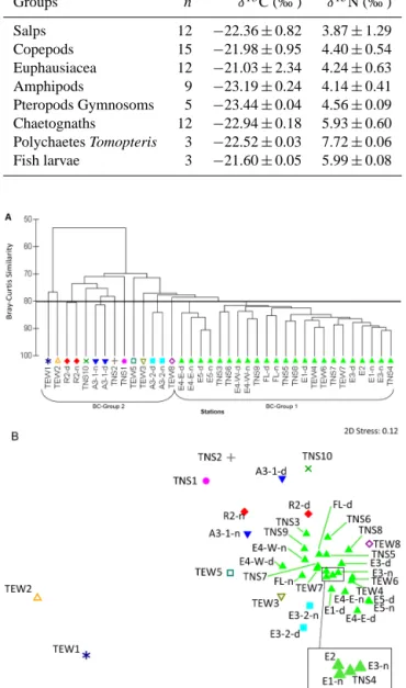
Table 3. Mean (±SD) stable isotope values of the main groups of organisms sorted in the largest size fraction (> 2000 µm). n is the number of samples analysed.
Groups n δ13C (‰ ) δ15N (‰ ) Salps 12 −22.36 ± 0.82 3.87 ± 1.29 Copepods 15 −21.98 ± 0.95 4.40 ± 0.54 Euphausiacea 12 −21.03 ± 2.34 4.24 ± 0.63 Amphipods 9 −23.19 ± 0.24 4.14 ± 0.41 Pteropods Gymnosoms 5 −23.44 ± 0.04 4.56 ± 0.09 Chaetognaths 12 −22.94 ± 0.18 5.93 ± 0.60 Polychaetes Tomopteris 3 −22.52 ± 0.03 7.72 ± 0.06 Fish larvae 3 −21.60 ± 0.05 5.99 ± 0.08
Figure 7. Dendrogram (a) and MDS plot (b) produced by the clus-tering of the 37 samples (28 stations, among them nine stations with day–night sampling) during KEOPS2 based on the density (ind m−3)of mesozooplankton taxa. Density values were fourth-root-transformed prior to analysis of the Bray–Curtis similarity ma-trix. The stress statistic for the MDS plot is 0.12.
its associated 2-D multidimensional scaling plot. This anal-ysis showed a high degree of similarity across the whole re-gion related to the initial phase of zooplankton development. The shelf stations presented the highest level of dissimilarity compared to the other stations.
The cluster dendrogram sliced at 80 % similarity distin-guished two BC groups: a first one (BC group 1, with more than 80 % similarity) grouping the oceanic stations within
the PF meander and including eastern stations east of PF (F-L and TW7), and a second group of dispersed stations (BC group 2, with less than 80 % similarity – differences in day–night sampling were not considered in this analysis), in-cluding the R2 station on the western side of the Kerguelen Plateau characterized by higher abundance of large calanoid copepods such as Rhincalanus gigas and Paraeuchaeta spp., the TEW1 and TEW2 stations, near the Kerguelen coast and dominated by Drepanopus pectinatus and bivalvia mero-planktonic larvae, the TNS1and TNS2 stations in Subantarc-tic Surface Water waters dominated by medium size cy-clopoid and calanoids and larval forms of euphausiids, the A3 and TNS10 stations in the southern part (see detail be-low), and stations TEW3, TEW5, TEW8, which were charac-terized by relative differences in very few taxa, compared to other stations of the TEW transect (high density of Metridida
lucens in TEW3, relatively lower density of Ctenocalanus citer in TEW5, and high density of Triconia sp. in TEW8).
3.4 Isotopic composition of size-fractionated
zooplankton and within zooplankton taxa
A wide range of δ13C (> 8 ‰ ) and δ15N (> 4 ‰) values were recorded among zooplankton size fractions and stations (Table 2). A slight general increase of δ13C with increasing size fraction was observed, while the difference was not sig-nificant due to wide differences between sites (F = 1.818,
p =0.132) (Fig. 8a). A significant increase in δ15N with in-creasing size was observed (F = 11.67, p < 0.001), particu-larly between the two smallest fractions (80–200 and 200– 500 µm) and the three largest ones (Fig. 8b). However, no sig-nificant difference in mean δ15N was apparent between the 500–1000 and > 2000 µm fractions, while the 1000–2000 µm fraction exhibited a slightly lower δ15N than the two others. Within each size fraction, no difference was observed be-tween mean day and night δ13C and δ15N values (p > 0.05 for both), in spite of differences at site level (Table 2). Thus, for both δ13C and δ15N values, the main difference occurred be-tween the two smallest size classes (< 500 µm) and the three largest ones (> 500 µm).
At the station level, mean δ13C and δ15N values differed. Station R2 presented the lowest mean δ13C (−25.26 ‰) and the highest mean δ15N (4.49 ‰), while stations F-L, TEW-8 and E4-E were characterized by the highest δ13C (> −21.2 ‰) and rather high δ15N values (> 4 ‰ ). All the other stations exhibited mean δ13C values (from −23.26 to
−21.76 ‰) and a wide range of mean δ15N values (from 3.63 to 4.25 ‰).
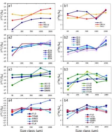
Differences in mean δ15N between small (< 500 µm) and large (> 500 µm) zooplankton size fractions were low in T-group 1 (0.3 ‰), increased in T-T-group 5 (0.6 ‰) and were highest at most stations located in the eddy (Fig. 9). This trend suggested higher food overlap among size fractions in zooplankton associated with phytoplankton group 1 and T-group 5, and more partitioned food resources in
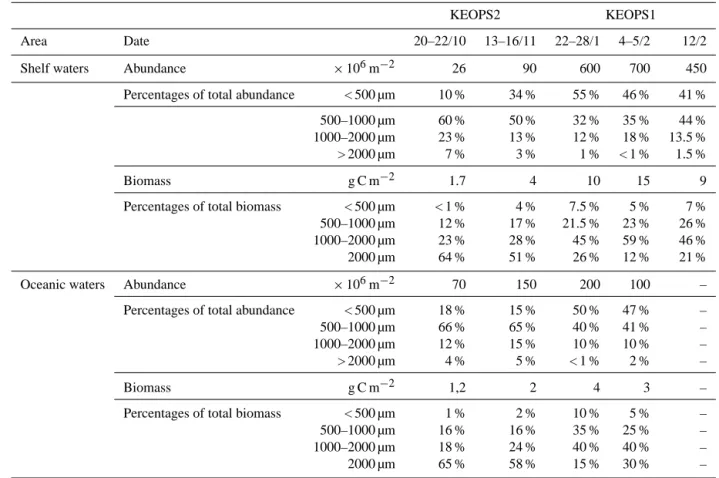
phytoplank-Area Date 20–22/10 13–16/11 22–28/1 4–5/2 12/2
Shelf waters Abundance ×106m−2 26 90 600 700 450
Percentages of total abundance < 500 µm 10 % 34 % 55 % 46 % 41 %
500–1000 µm 60 % 50 % 32 % 35 % 44 %
1000–2000 µm 23 % 13 % 12 % 18 % 13.5 %
> 2000 µm 7 % 3 % 1 % < 1 % 1.5 %
Biomass g C m−2 1.7 4 10 15 9
Percentages of total biomass < 500 µm < 1 % 4 % 7.5 % 5 % 7 %
500–1000 µm 12 % 17 % 21.5 % 23 % 26 %
1000–2000 µm 23 % 28 % 45 % 59 % 46 %
2000 µm 64 % 51 % 26 % 12 % 21 %
Oceanic waters Abundance ×106m−2 70 150 200 100 –
Percentages of total abundance < 500 µm 18 % 15 % 50 % 47 % –
500–1000 µm 66 % 65 % 40 % 41 % –
1000–2000 µm 12 % 15 % 10 % 10 % –
> 2000 µm 4 % 5 % < 1 % 2 % –
Biomass g C m−2 1,2 2 4 3 –
Percentages of total biomass < 500 µm 1 % 2 % 10 % 5 % –
500–1000 µm 16 % 16 % 35 % 25 % – 1000–2000 µm 18 % 24 % 40 % 40 % – 2000 µm 65 % 58 % 15 % 30 % – -28,0 -26,0 -24,0 -22,0 -20,0 -18,0 -16,0 0 500 1000 1500 2000 2500 δ13C (‰) 1,5 2,0 2,5 3,0 3,5 4,0 4,5 5,0 5,5 6,0 6,5 0 500 1000 1500 2000 2500 δ15N (‰) 80 200 500 1000 > 2000 80 200 500 1000 > 2000
Size classes (µm) Size classes (µm)
A B -28,0 -26,0 -24,0 -22,0 -20,0 -18,0 -16,0 0 500 1000 1500 2000 2500 δ13C (‰) -28,0 -26,0 -24,0 -22,0 -20,0 -18,0 -16,0 0 500 1000 1500 2000 2500 δ13C (‰) 1,5 2,0 2,5 3,0 3,5 4,0 4,5 5,0 5,5 6,0 6,5 0 500 1000 1500 2000 2500 δ15N (‰) 1,5 2,0 2,5 3,0 3,5 4,0 4,5 5,0 5,5 6,0 6,5 0 500 1000 1500 2000 2500 δ15N (‰) 80 200 500 1000 > 2000 80 200 500 1000 > 2000 8080 200200 500500 10001000 > 2000> 2000
Size classes (µm) Size classes (µm)
A B -16.0 -18.0 -20.0 -22.0 -24.0 -26.0 -28.0 1.5 2.0 2.5 3.0 3.5 4.0 4.5 5.0 5.5 6.0 6.5
Figure 8. Distribution of δ13C (a) and δ15N (b) of zooplankton across size fractions during KEOPS2. White symbols represent day; black symbols represent night.
ton T-group 2 and T-group 3, as indicated by a more even increase in δ15N with zooplankton size at these stations.
The smaller size fraction (80–200 µm) was differently composed according to stations, being dominated either by diatoms (A3-2, E-4W), foraminifera (A3-1), small copepods (R2), or a mixture of these groups (most stations). Cope-pods, eggs, thecosome pteropods foraminifera and small ag-gregates contributed to 200–500 µm fractions. The following size fractions (500–1000, 1000–2000 and > 2000 µm) were all dominated by copepods (60–95 %), but amphipods, eu-phausiids, appendicularians and chaetognaths increased in abundance from the 500–1000 to the 1000–2000 µm frac-tions. The largest size fraction (> 2000 µm) was dominated by Rhincalanus gigas and euphausiid larvae or juveniles. Large chaetognaths completed this large fraction.
Thus, differences in specific composition of size fractions, particularly the smallest and the largest, could result in iso-topic differences between stations within a size fraction. For example, when diatoms dominated the 80–200 µm fraction,
δ15N values were lower than when composed of foraminifera or small copepods (2–3 and 4–4.5 ‰, respectively).
Figure 9. Distribution of δ13C (left column, a) and δ15N (right col-umn, b) values across zooplankton size fractions for four of the five T-groups of stations identified by Trull et al. (2015) for phytoplank-ton. Station E4-E is included here in T-group 5 instead of T-group 2. From top to bottom: a1 and b1, T-group 1 (diamonds); a2 and b2, group 2 (triangles); a3 and b3, group 3 (dots); and a4 and b4, T-group 5 (squares). T-T-group 4 included coastal stations not sampled in the zooplankton analysis.
Groups of organisms individualized in the > 2000 µm frac-tion presented highly different isotopic signatures according to their main feeding behaviours (Table 3). Filtering salps presented the lowest δ15N (< 4 ‰), the mostly herbivorous copepods, amphipods, euphausiids, and pteropods interme-diate values (4 to 4.6 ‰), while predatory chaetognaths, fish larvae and polychaetes exhibited higher δ15N values (> 5 ‰). Thus, δ15N differences of the > 2000 µm fraction between stations resulted mainly from the relative contributions of these groups to bulk samples (e.g. higher proportion of salps and euphausiids at A3-2, and large chaetognaths at E5). Ac-cordingly, differences in δ13C values could be linked to dif-ference in both size and composition of the ingested food. The lower δ13C recorded in gymnosomes and copepods sug-gested the consumption of small phytoplankton particles, while the higher δ13C of euphausiids suggested a consump-tion of larger-sized phytoplankton. Higher δ13C in euphausi-ids compared to copepods was also observed in Arctic seas (Schell et al., 1998).
4 Discussion
4.1 Zooplankton development during the 2011 early
spring bloom and comparison with other seasons
In high latitudes, zooplankton first increase in abundance more than biomass in response to initial phytoplankton spring bloom due to stimulated reproduction of overwinter-ing adults of dominant copepods. This induces a lag-time in the grazing response of herbivorous zooplankton at the be-ginning of blooms, which further promotes the rapid phy-toplankton accumulation. Higher phyphy-toplankton concentra-tions then stimulate grazing by overwintering stages and new cohorts which results in build-up of zooplankton biomass. With the succession of new cohorts in full bloom conditions (> 0.8 mg Chl a m−3), continuous egg production and indi-vidual growth induce proportional increase of abundance and biomass.
Such a response of zooplankton to an early phase of the north-eastern Kerguelen bloom was observed during the La-grangian survey within the stationary meander of the Po-lar Front (stations E1 to E5, except E4-W, Figs. 2, 3 and 4). The average integrated Chl a concentrations were rather low (0.49 to 0.77 µg Chl a m−3)for these E stations and but slightly higher than the previous weeks – transects TNS and TEW- (Lasbleisz et al., 2014). The POC was constant in the surface layer up to the time of E3, with an average of 83 mg C m−3, and then slightly increased at E4 and E5 (with an average up to 109 mg C m−3) (Lasbleisz et al., 2014). Zooplankton densities increased from 60 × 103ind m−2 (E1-d) to 200 × 103ind m−2(E5-d) whereas biomass gradually decreased (excepted E4-E-n) from 2.3 g C m−2 (E1-d) to 1.7 g C m−2(E5-n). Two processes may favour the shift to-wards smaller size classes. Firstly, the contribution of the larger size classes to biomass decreased with time (Fig. 3) due to the reduction of initial standing stock of overwin-tering zooplankton by mortality and by investment in egg production. The dominant overwintering copepods
(Cteno-calanus citer, Rhin(Cteno-calanus gigas) are known to be strong
seasonal migrants able to spawn in early spring even at low chlorophyll concentrations (Schnack-Schiel, 2001; Atkin-son, 1998), i.e. before the full bloom conditions. Moreover, smaller copepod species and copepodids of large copepods may better exploit these low food concentrations (Atkin-son et al., 1996), allowing individuals to develop and grow, whereas large copepods are food limited.
The response to chlorophyll increase in waters above the plateau (station A3 in Fig. 4c) was proportional in abundance and biomass (threefold higher at A3-2 than at A3-1). Las-bleisz et al. (2014) mention that the Chl a increase at station A3-2 was accompanied by an increase of the Phaeo : Chl a ratio, reflecting a potential higher grazing activity. The meso-zooplankton at A3-2 (see Fig. 6) presented a grazer com-munity structure able to feed on a wide spectrum of cells from small diatoms to phytodetritus aggregates, as observed
quickly remove the smaller planktonic forms (below 20 µm). The larger zooplankton size fractions were a mixture of effi-cient grazers on large diatoms (> 20 µm), omnivores and de-tritivores able to feed on aggregates, and carnivores consum-ing micro- and mesozooplanckton.
The mesozooplankton biomass stocks observed at the beginning of the KEOPS2 cruise (Table 4) were around 1.7 g C m−2 above the plateau (A3) and 1.2 g C m−2 in oceanic waters (TNS transect). Oceanic biomass slightly in-creased during the cruise, except the biomass observed in the eastern bloom (station F-L) in the Polar Front zone (above 4 mg C m−2), and station A3 also presented biomass around 4 mg C m−2 at the end of the survey. These differ-ent results during KEOPS2 suggest that the zooplankton community is able to respond to the growing phytoplank-ton blooms earlier on the plateau than in the oceanic waters, where complex mesoscale circulation stimulates initial more or less ephemeral blooms before a broader bloom extension. Due to our constrained sampling for oceanic stations, it was not possible to determine whether the observed zooplankton biomass variability between oceanic stations was linked to enhanced local production (except for stations near the per-manent Polar Front sustaining high level of production). Our results in the quasi-Lagrangian survey within the meander suggests that the heterogeneous primary production linked to oceanic mesoscale activity in the early bloom phase may stimulate the production of new zooplankton cohorts, with-out sustaining individual growth, slowing down the built-up of new zooplankton biomass. In addition, potential preda-tion on mesozooplankton by euphausiid populapreda-tions was ex-pected, from observations of the increasing contribution of euphausiid larval stages in our Bongo net samples (see Fig. 6) and of long faecal pellets in gel traps (Laurenceau-Cornec et al., 2015).
In contrast, stations F-L (06 November) and A3-2 (16 November) presented the highest biomass (maintained below 5 g C m−2)observed in November (Figs. 4 and 5) and a similar ratio of abundance to biomass, around 20 × 103ind per g C (Fig. 4c) and a lower contribution of smaller size fractions (ESD < 1000 µm) to total biomass comparatively to station E5. These characteristics could be the results of a phytoplankton-sustained zooplankton development over the previous weeks.
4.2 Comparison with previous results
If we group our observations of KEOPS1 and KEOPS2 (Ta-ble 4), the zooplankton seems to continuously increase from mid-October to early February, with a ratio higher on shelf
70 to 85 %), with the production of calanoid copepod lar-val stages and large numbers of cyclopoid copepods, whereas the increase in biomass is mainly due to the fraction 1000– 2000 µm with calanoid copepod late larval stages (with a con-tribution doubling from spring to summer). The taxonomic composition did not show major differences between shelf and oceanic waters, except that the contribution of copepods to the whole mesozooplankton was higher in oceanic waters than on the shelf, and these taxonomic patterns were quite similar between the KEOPS 1 (see Fig. 7 in Carlotti et al., 2008) and KEOPS2 survey (Fig. 6).
The use of different laboratory technologies (Lab OPC during KEOPS1 and ZOOSCAN during KEOPS2) to op-tically measure and size plankton organisms from net haul samples must be considered. In their comparative study be-tween LOPC and ZOOSCAN, Schultes and Lopes (2009) found good agreement in the normalized biomass size spectra (NBSS) for particles in the size range of 500 to 1500 µm in equivalent spherical diameter (ESD). Several disparities for smaller and larger particles size range in their study were due both to in situ sampling (LOPC and net have different sam-pling efficiencies), in situ vs. lab counting (LOPC counts any particles, not only zooplankton, with potential overlapping between particles, whereas ZOOSCAN samples are carefully distributed on a scanned window), etc. Our present com-parison of estimated abundance and biomass for KEOPS1 and KEOPS2 is based on similar sampling protocols with a 330 µm mesh net on the Bongo frame, and in both cases a delicate laboratory protocol. The flow-through system used with the Lab-OPC for KEOPS1 samples was controlled to avoid coincidence of organisms counted by the laser (count rate at 20 particles min−1; see Carlotti et al., 2008) and or-ganisms were carefully separated on the ZOOSCAN window for the KEOPS2 samples. In both studies, a large number of individuals were counted (1000 particles per samples) to cor-rectly count and size larger organisms. Finally, the lower and higher range of counted and measured zooplankton organ-isms are mainly due to the 330 µm mesh net efficiency, and the abundance and biomass results of both studies might be compared.
In addition to the recent survey of the CPR data for the re-gion (see in Introduction), which shows the strong develop-ment of mesozooplankton abundance in October–November, the overall results of KEOPS 1 and 2 in terms of seasonal changes in abundance and biomass values are highly con-sistent with the information provided by Semelkina (1993) and Razouls et al. (1996, 1998). During the SKALP cruises, all around the Kerguelen Islands (46–52◦S, 64–73◦E), Semelkina (1993, her Table 1) observed an increase from