An application of nonlinear resistive networks in computer vision

An Application of Nonlinear Resistive Networks in

Computer Vision

by

Bikui Chen

Submitted to the Department of Electrical Engineering and Computer

Science and Department of Nuclear Engineering

in partial fulfillment of the requirements for the degrees of

Master of Science in Electrical Engineering and Computer Science

and

Master of Science in Nuclear Engineering

at the

MASSACHUSETTS INSTITUTE OF TECHNOLOGY

May 2000

@Ma1rb11Ptts

Institute

A uthor ...

...

Department of Electrical Engineering and Computer Science and

Department of Nuclear Engineering

C ertified by ...

...

d Computer Science

Thesis Supervisor

JUL

3 i 2001

BARKER

Certified t

Richard Lanza

Senior Research Scientist of Nuclear Engineering

Thesis Supervisor

Read by ...

Principal Resea

Ichiro Masaki

Laboratory

i6sis Reader

Accepted by ....

...

Arthur C. Smith

Chairman, Department Committee on Gracdat? StudeAA, EECS

Accepted by ...

An Application of Nonlinear Resistive Networks in

Computer Vision

by

Bikui Chen

Submitted to the Department of Electrical Engineering and Computer Science and Department of Nuclear Engineering

on May 3, 2000, in partial fulfillment of the requirements for the degrees of

Master of Science in Electrical Engineering and Computer Science and

Master of Science in Nuclear Engineering

Abstract

In this thesis, an improved optical flow algorithm is presented, as well as a hard-ware called "Tanh" component. The new approach performs an optimization that reduces the error at spatial discontinuities, and increases the computational speed using analog circuit implementation.

Simple simulation of this design is tested using HSPICE. We also build a simulator for a complicated circuit using C, which focuses more on speed, and less on transient. For image smoothing and segmentation problems and optical flow problems, a series of test images are fed to both the resistor network and the so-called "TANH"

network to determine how effective the Tanh network is in image analysis.

Thesis Supervisor: Berthold K. P. Horn

Title: Professor of Electrical Engineering and Computer Science

Thesis Supervisor: Richard Lanza

Acknowledgments

I would like to express my deepest gratitude to my supervisor, Professor Berthold K. Horn, for giving me the opportunity and support to work on this thesis, for providing me with crucial guidance and encouragement throughout years, and for serving as a model of an enthusiastic teacher and a dedicated scientist. I am also grateful to Dr. Richard Lanza, my thesis co-supervisor, for providing invaluable insight, ideas, and support. I have learned much from their expertise and am grateful for the time they have devoted to me.

This work has benefited from many discussions with Professor John L. Wyatt about non-linear networks, Professor Hae-Seung Lee about analog circuit design, Pro-fessor Rahul Sarpeshkar about non-linear analog circuit design and Dr. Christopher Terman about non-linear circuit simulation. I thank all of them for their enthusiasm,

patience, and advice.

I would like to express my gratitude to all the people from my research group, Dr. Ichiro Masaki, Paul Fiore, Nicole Love and Yajun Fang, for their help and invaluable advice in the past three years.

I would also like to thank all my friends in MIT and elsewhere for the great moment we have shared in the past years, especially thank Benjamin Walter, for his advice and help in thesis revising.

I would like to express my deep love to my family, especially my parents, who have granted me unconditional love throughout my life; my sisters Bizhou and Jin, my brothers Bihui and Juhui, who have given me all kinds of support in both my career and my life.

Finally and most importantly, I would like to thank my girl friend, Xiang Xian, for her love and encourage.

Contents

1 Introduction 9

1.1 Optical Flow . . . . .. .. 9

1.2 G oal . . . . 10

1.3 Thesis Organization. . . . . 10

2 Theory and Algorithm 12 2.1 The Optical Flow Problem . . . . 12

2.2 Previous Work . . . .. . . . 17

2.3 Our Work . . . .. . .. . .. . .. 17

2.4 Comparison of Smoothing Terms . . . . 23

3 Hardware Design and Simulation 25 3.1 Hardware Design . . . . 25

3.1.1 G oal . . . . 25

3.1.2 Previous work . . . . 25

3.1.3 Tanh Resistive component . . . . 26

3.2 Simulation . . . . 28

3.2.1 Transfer Function of TANH Circuit . . . . 28

3.2.2 Solving Nonlinear Circuit . . . . 30

3.2.3 Solving Sparse Matrix . . . . 31

3.2.4 Image Segmentation Simulation . . . . 37

4 Conclusion 51 4.1 Summary ... ... 51 4.2 Recommendation . . . .. . . . . . . .. . . 51

List of Figures

1-1 Structure of Computer System . . . .

2-1 Optical Flow Field . . . . 2-2 1-D BCCE Equation . . . .

2-3 Concave Smooth Function . . . .

2-4 Ideal Transfer Function of Interconnection .

2-5 Resistive Grid . . . .

2-6 A Node in the Resistive Network . . . . 2-7 Comparison of Four Smoothing Terms . . . 3-1 3-2 3-3 3-4 3-5 3-6 3-7 3-8 3-9 3-10 3-11 3-12 3-13 3-14

Simplified Mead's Saturating Resistor . . . . Simplified TANH circuit . . . . Detail of TANH Circuit . . . . Transfer Function of TANH circuit (from HSPICE) . . . .

Transform a Nonlinear Resistor into Linear Components R esistor Chain . . . .

1-D Voltage Input . . . . Comparison of Smoothing Effect (1-D) . . . . Image Input (64x64) . . . . Simulation Result of Image Segmentation . . . . Comparison of Smoothing Effect . . . . 2-D Gaussian Filters . . . . Pixel Cube Used to Estimate the Three Partial Derivatives Input Images of Optical Flow Simulation . . . .

10 13 14 19 20 21 21 24 . . . . 26 . . . . 26 . . . . 27 . . . . 29 . . . . 31 . . . . 37 . . . . 38 . . . . 39 . . . . 41 . . . . 42 . . . . 43 . . . . 45 . . . . 46 . . . . 47

3-15 Simulation Result of Optical Flow Algorithm with Tanh Network and Resistor Network . . . . 48 3-16 Comparison of Simulation Results from the Tanh Network and the

List of Tables

3.1 1-D Image Segmentation Error Comparison between Tanh Network and Resistor Network . . . . 40 3.2 Optical Flow Error Comparison between Tanh Network and Resistor

Chapter 1

Introduction

Twenty years have passed since Professor Berthold K.P. Horn and Brian Schunck published their influential paper[6] on the calculation of optical flow. Since then, a substantial amount of research has been devoted to finding ways to calculate optical flow more efficiently and more accurately. Despite volumes of research that have been

published on this topic, the best current approach remains computationally intensive, because the vector field must be computed pixel by pixel. In the thesis, an analog resistive network is presented that will increase the processing speed and reduce the error at discontinuities.

1.1

Optical Flow

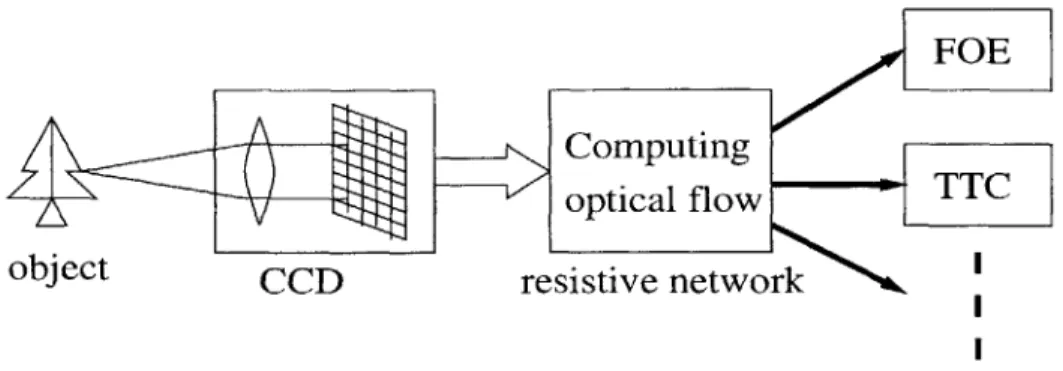
We can get much more information from an image sequence than from a single image. When a camera has motion relative to an object, a change of the brightness pattern in the image can be observed. This is called optical flow[5]. If we assign a velocity vector to each point in the image, we can get a motion field[5]. Since optical flow is a very good approximation of the motion field, optical flow extraction has been proposed as a preprocessing step for many high level vision algorithms. Knowledge of the optical flow field can provide the basis for the calculation of important parameters such as the Time-to-Collision (TTC) and the Focus-to-Expansion (FOE).

FOE Computing

optical flow TTC

object CCD resistive network

Figure 1-1: Structure of Computer System

Figure 1-1 shows the structure of a computer vision system. The Charge-Coupled Device (CCD) grabs the image of objects, converts them into voltage signals, then feeds them into a resistive network. The resistive network computes the optical flow as the intermediate result, and provides the input for other applications, such as com-puting TTC and comcom-puting FOE. Our work mainly focuses on the implementation the resistive network.

1.2

Goal

In this research, two approaches are considered. One is to implement the optical flow algorithm using an analog resistive network, which can increase speed and save power significantly. The other is to improve the algorithm, and design a new nonlinear resistive component, which can reduce the error near the spatial discontinuity, and simultaneously solve the local minima problem[1].

1.3

Thesis Organization

Algorithm improvement and hardware implementation are presented separately. Chap-ter 2 will introduce the theoretical framework, the optical flow algorithm and assump-tion that are used in this thesis. Based on this framework, Chapter 3 describes the hardware implementation, hardware architecture and the so-called TANH non-linear

resistive circuit. Results obtained using software simulation are then presented. Fi-nally, Chapter 4 closes with conclusions and future work.

Chapter 2

Theory and Algorithm

2.1

The Optical Flow Problem

"Brightness patterns in the image move as the objects that give rise to them move. Optical Flow is the apparent motion of the brightness pattern. Ideally the optical flow will correspond to the motion field."

[5].

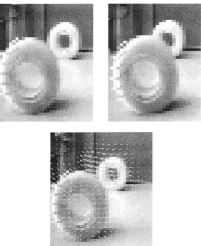
In Figure 2-1, the top two images are taken at the beginning of the end of a short time interval. We can tell that the two donuts are moving toward each other, because the area of overlap is greater in the second image. In the bottom image, the arrows show the optical flow field, with the velocity at each point being proportional to the length of the arrow. We need to pay attention to two things here. The first is that the optical flow field gives useful information about how those objects are moving. The second is that some non-zero velocity vectors appear in the static background. This is happened because in computing optical flow we assume that the velocity varies smoothly, which is not true at spatial discontinuities. The result is that the velocity vector dies slowly, which causes in significant error. In this thesis, we are going to focus on this problem, and look for an effective solution.

There are several methods to compute the optical flow field from given images, one of which is a gradient-based method. We can assume the lighting condition does not

slope:Ex

At

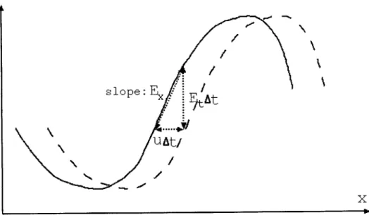
Figure 2-2: 1-D BCCE Equation

change. If the time interval between two frames of image is very small. Under these conditions, we can derive the Brightness Constant Constraint Equation (BCCE)[5]. Figure 2-2 shows the 1-D case.

In figure 2-2, u is the velocity along the x direction, Ex is the derivative of bright-ness in the x direction, Et is the derivative of brightbright-ness with respect to time.

After time At, the brightness curve changes from the solid curve to the dashed curve. There are two ways to calculate the brightness change of a particular point.

(u - At) -(Ex) and -At - Et. Equating these, we obtain

(u -At) - (Ex) = -At -Et (2.1)

or

Similarly, we can obtain the equation for the 2-D case[5l,

u.Ex+v.E~y+Et = 0 (2.3)

where u is the velocity in the x direction, v is the velocity in the y direction. This equation holds for each pixel.

We get one equation with two unknown variables. We need another constraint, which is a regularization term, to solve it. We can add a rigid body assumption, because most objects we deal with are rigid body. When objects are rigid bodies, the motion field varies smoothly across the image. We therefore seek to minimize a measure of departure from smoothness.

es = ((u2+u ) + (v2+ v2)) dx dy

The integral of square of the magnitude of the gradient of the optical flow. The error in the brightness constraint equation,

Cc =

J J

should also be small.

Overall, the optical flow problem is to minimize the total error of these two terms.

E ef +A- e, (2.4)

J

(u. - E+ v- Ey + E) 2 _{dx dy + A}

J

dy

((u

-Ex

E = ef ij + A - es ij

Ex i + v,, -Ey i + Et ij)2 + A(U2

ij + U2 ij + V2 ij + V2 j

Differentiating the error with respect to uij and vij yields

OE

= 2A(ij - Uig) + 2(uigE ij OFi

= 2A(v2i, - UTj) + 2(uigEx ij,

vi1

+ Vij Ey ij + Et i,)Ex i = 0

+ viEy ij + Et ₂,)E is = 0

From its Euler-Langrange Equations, we get,

(A + Ex ij)uij + Ex E ,j vij = A-iU, - Ex _{2 3}Et

E 2,3Ey ijui, + (A + E2 4,)vij = A7jj - Ey 2 3Et jj

Where Uj, and Uj are local average of u and v. These equations can be solved with an iterative scheme[5] as t'U.l =tt;an 2,3 2,3 n+1 _-n 2,3 2, E 213. + liEy ij + Et _{ij F} U,3 ijExj + 7jEY 4,j + Et jj A+ E2 i,+ E2 EY i'j -n_Mi'j _Fn +- + Y j +₁ 4 S, + + vj j-1 + ~±1 4

From the recursive formula, we can see that when it converges, E EE Zig+ Ej+

(2.6) where (2.7) (2.5)

=EE ((Uig

Et i,y = 0, which is exactly the brightness change constraint equation. Then uij = Uij and vij = vij.

2.2

Previous Work

Solution of optical flow problem has two intrinsic difficulties. Firstly, it is computa-tionally expensive, because the algorithm involves iterative pixel-wise computation. Secondly, it introduces the smoothness term, which assumes the motion field varies smoothly. In Figure 2-1, the error that can result from this assumption is visible in the spurious background motion vectors.

There are several hardware implementations of optical flow algorithm, such as Tanner and Mead's Optical Motion Sensor[7], and Alan Stocker's optical computation circuit [14].

Strictly speaking, Tanner and Mead's chip is not a implementation of the optical flow algorithm, because they only produce a single unified global velocity instead of a pixel-wise velocity field. Alan Stocker improved Tanner and Mead's work, but his approach still suffers from the local minima problem, which we will discuss in Chapter 3.

There is also related research done on the image smooth and segmentation problem [4][8][10][11][13], such as Professor John Wyatt[1][2][9], Dr. Pietro Perona and Dr. J. Malik's resistive fuse[12], Dr. John Harris' tiny-tanh resistive element[3].

2.3

Our Work

Our goal was to design an algorithm that reduces error at spatial discontinuities, and allows large velocity gradients in those areas.

Another important problem in computer vision is the image smoothing and seg-mentation problem, which mathematically is to minimize the object function,

E = (u - e)2 _{dxdy+ A - (u2+ u ) dx dy}

= F(ule) + S(u)

where u is the smoothed output, e is image input. The object function of optical flow problem is

E =

ff

= F(u, vlEx, Ey, Et) + S(u, v)

We can see some similarities between these two functions. They both consist of two terms, a fidelity term F and a smoothness term S. F is trying to get the best estimation of some parameter from input, and at the same time, S is smoothing the estimate[15].

In the recursive algorithm for the optical flow problem, the effect of the regular-ization term is to smooth the motion field. However in our approach, we want to preserve the edge features while smoothing out the noise. So I apply the network we designed to both the image smoothing and segmentation problem, and the optical flow problem.

A great deal of work has been done to improve the performance of image smooth-ing algorithms. One approach is to use a different smoothsmooth-ing term. The most common smoothing term is a quadratic smoothing function, such as f f (z!

+

)

(Iu

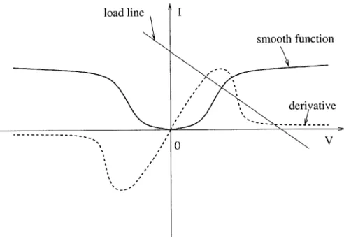
In Figure 2-3, the solid line represents the smoothing function, and the dashed line is its first order derivative. Wyatt, Perona and Malik also implemented the smoothing function using a resistive-fuse circuit, which produces very good result in

load line

smooth function

derivative

Figure 2-3: Concave Smooth Function

some images.

However, their circuit has local minima problem[1]. The derivative of the concave smoothing function is the V-I characteristics function of the resistive-fuse element. The straight line in figure 2-3 is the load line in the physical circuit. It intersects with the V-I curve more than once. Thus, there are multiple solutions to the object equation. The circuit may just converge to a local minimum.

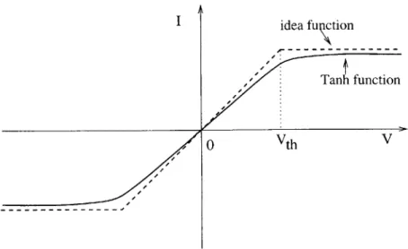
What do we expect the behavior of a nonlinear resistor to be? When the input voltage difference across its two nodes is small, we assume that they are from pixels corresponding to the same object. In this case, the resistor should act like a normal resistor, so that it can conduct the filtering work. When the voltage difference is large, we may conjecture that they are from different objects. The resistor should cut off communication between these two neighboring nodes. There are at least two methods to implement this. We can cut off the current completely, as in John Wyatt

and Malik's work, which is known to suffer from local minima[1]. We can also instead limit their relationship by limiting the current flow.

I idea fu tion

Tanh function

S0 Vth V

Figure 2-4: Ideal Transfer Function of Interconnection

connection component. When the voltage is smaller than Vth, the current increases

linearly, just as in a normal resistor; when the voltage exceeds Vth, the current stops

increasing. The ideal transfer function is not physical implementable, because its first

order derivation at Vth is not continuous. We can use the hyperbolic tangent function

(tanh) to approximate it. It is shown as the solid line in figure 2-4. The Tanh function is even better, because its first order derivative is always continuous.

Figure 2-5 shows the basic structure of a resistive network in our approach. And

Figure 2-6 shows detail at a node in the grid.

Each node is connected to its four neighbors by four resistive elements. At each node, a voltage-controlled current source injects current, which is zero when the circuit settles to its final state.

We now prove that the TANH circuit network will reach the optimal solution for

the optical flow problem when the circuit settles. Similarly, we also prove that it solves the image smoothing and segmentation problem.

One concept is very important in nonlinear network analysis. That is the Co-Content of a resistive element[15]. For a resistor with a voltage-controlled constitutive relation

Figure 2-5: Resistive Grid

I _i~j Si.j+1

0i y\ -AAA9--- V

V i,j-1

Sg (v),

the co-content is defined as

J(v) = fo g(v')dv'.

In particular, for a linear resistor, the co-content is simply half of the dissipat-ed power. Although power and co-content have the same units, they are distinct in non-linear circuits. According to the Minimum Co-Content Principle[15], while the minimum power dissipation property fails for circuits with nonlinear resistive components, the total co-content is minimized instead[15].

If we use the integral of the TANH function as the smoothing term, then the error function of the optical flow problem becomes

E J J (u.E +v . E + Et)2 ddy

+Af ( tanh(v)dv+ tanh(v)dv

+ tanh(v)dv + tanh(v)dv)dxdy

Its discrete case is

E = EE[(ui,j - Exij + i -Ejj + Eti )2 (2.8)

+ A( tanh(v)dv + tanh( )dv

/

fo+ -vi,j

+ tanh(v)dv +

j

Et+lJ)

₊

_tanh(

7 j+1) (2.9)

i 0A(tanh( 6 6

+ tanh( Ui Ui1)) + 2(uij Ex ij + v, Ey ij + Et i,3)Ex ij

OE V-j --vi+1~ v -17 V- Vi -v j+1

= 0 = A(tanh( 6 + )+tanh(vij - v' ) tanh( ' i'+)

ovg6 6

+ tanh( Vij - vij _)) + 2(u, Ex ij + v,, Ey ij + Et i,) E,5

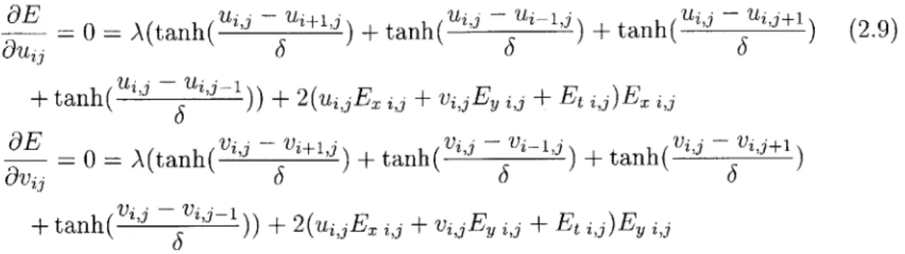
These are transcendental equations, so that we can not get analytical solutions. But we can design a physical circuit, which will satisfy these equations when they are in stable state. Let's use the u component as the example.

We can build a resistive grid with TANH components. One node from that grid is shown in the figure 2-6, the voltage of the central node is uiJ, and its neighbors' voltage are ui_,j, ui+,,, ui,j-i, ui,j+1. They are all connected by the TANH components, which satisfy I =A tanh(!). A voltage-controlled current source Iij is connected to this node. The current it injects is 2(u,jE, ij + vi, Ey i, + Et i,)Ey i,. Each node satisfies the Euler-Langrange equation, and the co-content of this nonlinear resistive network is the same as the error function for the optical flow problem. According to the Minimum Co-content Property, the voltage distribution ui,, and vij at the stable state minimize the error function. Because the tanh( function is a strictly increasing convex function, the circuit always settles at the unique optimal point in the stable state.

2.4

Comparison of Smoothing Terms

Figure 2-7 compares four known smoothing functions. What characteristics should a good smoothing term have?

(a) When AV is small, it acts similar to a linear resistor, and far from the line I=kV (in this case, the current will saturate immediately at 0+ and no smoothing

0 smooth ... Linear Resistive Network Resistive Fuse Network ...-- _Tiny-Tanh Circuit Network Tanh Circuit Network - . - ---.- ... --.. ...

Figure 2-7: Comparison of Four Smoothing Terms

(b) When AV is large, it should be small, in order to preserve the edge features. Observing Figure 2-7, we can see that the Tanh function is nearly linear for small Av, so that it has more smoothing effect when Av is small, which we suppose to correspond to noise, and has less smoothing effect when Av is large, which occurs at velocity discontinuities. In this sense, integral - tanh function beats both quadratic

function and absolute-value function as the regularization term. V

Chapter 3

Hardware Design and Simulation

3.1

Hardware Design

3.1.1

Goal

In our design, the resistive network is actually a grid of resistive components. Resistive grids are well known as an efficient method of providing local interaction between cells with minimum requirement in terms of space and interconnection. In this paper, we

will investigate the application of nonlinear resistive networks to vision problems. Ideally, we would like the resistive components to act like linear resistors for small potential differences, and cut off when voltage is large. We also desire the circuit to be compact, since we are going to duplicate it for each pixel, and integrate them into one single chip. It should also work robustly in case of transistor mismatching. One of the easiest function of this kind is TANH function. So that we choose TANH as our solution for this problem.

3.1.2

Previous work

The next step is to implement the nonlinear resistive component. Dr. Carver Mead designed a saturating resistor[7]. It can be simplified to two transistors and two

vi

V2

in1

M1

M2

in2

Figure 3-1: Simplified Mead's Saturating Resistor

V

inI

M1

M2

in2

Figure 3-2: Simplified TANH circuit

V1 and V2 provide offset voltage with value of a Vgs. When jVini - Vin2 is small, both MI and M2 are in linear region, they act like linear resistor. When jVj1 - Vin2j is large - let's assume Vini is larger than Vn2, - MI is in linear region, and M2 is in

saturated region, the current flowing through is limited by M2, and vice versa when

Vin2 is larger than Vin1[91.

3.1.3

Tanh Resistive component

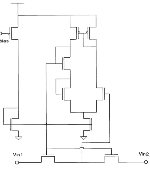
Following a suggestion by Professor Rahul Sarpeshkar, we combine the function of those two voltage sources into a single source. The voltage-current characteristics curve of the resulting circuit is a good approximation of the TANH function.

The detail of TANH component is shown in Figure 3-3. V1 bias controls the

conduc-tance of this circuit in the linear region. Higher values of Vbias lower the conducconduc-tance

YE-Vin1 -3 V2

Figure 3-3: Detail of TANH Circuit

0-=

-which will cause the Vgs of the bottom two NMOS to drop. Then the current flowing through the right part of circuit will decrease also. This causes that all the Vgs on the right part of the circuit to drop. As the voltage that the upper part of the circuit provides drops, the conductance of the bottom two horizontal NMOS decreases. We tried several other designs, but this one has an important virtue. The current flowing in from one side is always equal to the current flowing out from the other side. We will not have current leakage or transistor mismatching problem.

3.2

Simulation

We use several methods to simulate our implementation of the algorithm. We use HSPICE to simulate the TANH resistive component and grids with less than 20 TANH components. For grid including more than 20 TANH resistive components,

we simulate using C/C++ and the transfer function of TANH circuit.

3.2.1

Transfer Function of TANH Circuit

We use HSPICE to simulate the TANH circuit we described in Chapter 3. Figure 3-4 is the HSPICE simulation result of the TANHcircuit transfer function.

In this simulation, we set one side of input to 3.OV, and change the voltage on the other side from 1.2V ~ 5.OV. We can see that when AV is lower than 0.3V, current I changes linearly, which is like a normal resistor. When AV is higher than

0.3V, current I starts to increase more slowly with the increase of AV. Furthermore,

after a narrow transient region, the rate of increase drops significantly. The transfer function looks like a Tanh() function.

Because HSPICE is very slow when simulating a complicated circuit, we use the transfer function instead of the real circuit in simulations of larger networks. We sample 50 points from the HSPICE simulation result, and use MATLAB to do second order interpolation, producing an array of 1000 samples of TANH transfer function. We use this transfer function in all the simulations later on. We can use the formula

I - - - -- - - - -- -- -- - - - -- - - --- - - - --- - - - --- - - --- - - - -- - - -- - - -- - - -- - - - - -- -- - - - -- - - - ---- --- ---I - -T -- 11 --11 - I -- -- -- -- -- -- -- -- -- -- -- -- -- -- -- -- -- -- -7 -- 7 -- i t - - - -- -- --- -- ---- -- -- -- ---- -- -- -F 7 T r 7 7 7 - - -- - - - - - - - -- -- --- - - -- - - - -T - -- - - - -- - - - -- - - - - - - --- -- -- ---- -- --- ---- -- - - - -- -7 T -7 7 7 7 - - -- -- -- -- -- --- - -- - -T -T T 7 -- -- ---- - -- -- ---- - - -- - - - -7 7 - - - --- - - - - - - - -1.2 1.4 1.6 1.8 2 2.2 2.4 2.6 2.8 3 3.2 3.4 3.6 38 4 4.2 4.4 4.6 4.8 5 x (11.) (VOLTS) ... ... ... ... . . . ... W.- SKMb.1 DDAOI( i.-) X-800. -55OU -501D. -450. -400u -350u -300u -250u -200u -150u -I u -sou -0 -50u -100U -150. -200u -250u -300U -350u -400u -450u -500U -550u -500U -850u ,r2LrqH Nr-x

1(a) = V[n] * (n + I - a) + V[n + 1] * (a - n) (3.1)

n E N, n <a < n + 1

to calculate the current I when the input voltage a is not one of the given samples. When simulating a nonlinear resistive network, we are faced with two problems, solving nonlinear circuit, since the TANH circuit has nonlinear transfer function, and solving sparse matrix, because each component only has connections to a few neighboring nodes.

3.2.2

Solving Nonlinear Circuit

In order to solve nonlinear equations using a matrix, we need to first linearize those equations. To linearize, we use the Newton-Raphson algorithm. For a nonlinear

resistor, its current I and voltage V satisfy I = f(V). The Taylor Series Expansion

of this equation about the operating point vo is

i = f(v) =f(vo)+ f '(vo)(v vo)+o(v -vo)2

We can derive the recursive scheme based on its Taylor Series Expansion,

i + f (v(+ 1)) f (v(')) + f ' (V(')) (V(+ 1) - v() (3.2)

= f '(v('))v(+ 1) + (f ((') - f '(V(/ ))

= f'(v('))v(') + I(v(1))

where I(v(M) = f(v(M) -f '(V(1)V(1.

Then we can replace a nonlinear resistor with a normal resistor and a voltage-controlled current source in parallel (see Figure 3-5).

+ O i=f(v) - 0 V + 1+1 .1+1

it

Figure 3-5: Transform a Nonlinear Resistor into Linear Components

The value of resistor is the first order derivative of transfer function

f

f

3.2.3 Solving Sparse Matrix

Node A in the resistive grid is connected to four neighbors B, C, D, E with four nonlinear resistive components. The conductance between node A and its neighbors are gAB, 9AC, 9AD, 9AE. It is also linked to load or ground with a normal resistor R.

Following Kirchoff's Voltage Law, we get equation:

VA - (YAB + 9AC + 9AD + 9AE +1/R)

-B 9AB - VC 9AC - VD 9AD - E 9AE A (3.3)

We can gather all the equations and write the result in the form

Element gij in G, shows the conductance between node i and node

j,

voltage at the nodes, and nxl represents the current source associated with each node.

If we have a resistor grid, with N x N nodes, we label each node with integers 1, 2, 3, 4, ... , N x N. Each node in the grid has connection to at most 4 of its neighbors. So G is a highly sparse matrix, with dimension (N2 x N2), it has at most five lines

of non-zero elements diagonal. A recursive methods yields an efficient solution to the sparse matrix, provided we can guarantee convergence. The positive conductance of those resistive components ensures that the recursive algorithm converges.

We are going to use Gauss-Siedel Recursive methods to solve these equations. If we divide matrix G into three matrixes, G = D - L - U, the recurrence is

(3.4) where U = -911 922 9nn 0 912 0 91n 92n 913 923 0 --- gn-In 0 0 921 931 9n1 0 932 gn2 0 0

Below is the proof of the convergence. Lemma A: If matrix Gnxn satisfies Igiij > Proof:

E jgij, then det(G) > 0.

1<j<n,ioj

Let's assume det(G) = 0, then there is nonzero solution for equation Gx = 0. We denote the solution as

x = (x1, x 2, X3, ... , n)T and IxkI = max Ixil # 0

1<i<n From Gx = 0, we get n SgkjXi = 0, then, j=1 n |gkkxkl = gk3jX j=1,j4k | gkJ|x j xi| j=1,j~k n IgkklI < E IgkjI j~1 ,jAk

the assumption: Igi > E Igij i/jn Theorem: If matrix G1x, satisfies Igiij > E

I<j<n,i#j

its recursive matrix R = (D - L)-U satisfies JAI < 1.

Proof:

, so we know that det(G) 7 0.

Jgjj, all the eigenvalues, A, of

In the equation Gnxn-Vx 1 = Inx1, we know that I gi 0(i = 1,2, ..., n) and IgiiI >

E Igij 1. The recursive matrix for Gauss-Siedel method is R = (D - L)-'U. Its

e<j<niaj

eigenvalues should satisfy

det(AI - R) = det(AI - (D - L)--U) = det(D - L) -(3.5) det(A(D - L) - U) = 0 that equals to =,J9kj jr~1,jAk

Let's denote C = A(D - L) - U = )gi 912 913 A9_{2 1} A9_{2 2} 92 3 Ag31 Ag32 A933 'Mini Agn₂ i-1 n E JAgijl + E

j=1 j=i+1

Igii

Z

from Lemma A, we know det(C) = det(A(D - L) - U) -L 0, Therefore, all A must

satisfy JAI < 1. In our problem, the conductance matrix has the form

[

Only five lines of non-zero elements appear in the diagonal direction. Each row of the conductance matrix corresponds to an equation in the form of equation 3.3. Because

-.-- ₉ 1n -..- 9 2n if JA > 11 Agnn-1 Agnn where 1/r 0 0 1/r nxn 0 0 0 0 93n

all the elements have positive conductance, for matrix G, those elements along the diagonal are larger than the sum of all other elements in the same row. That is to say,

IgiiI > E lgikl

1<k<NxN

iAk

Then it fits Theorem B, so that the absolute values of all the eigenvalues of its recursive matrix (D - L)-'U are less than 1. We know that the recursive method converges if and only if the absolute value of all the eigenvalues of the matrix are less than 1. Therefore the Gauss-Siedel method converges for this problem.

For the image segmentation problem, the conductance should satisfy the equation,

G - R Vout Inode(37

g2[0] g3 gl[1] g2 ... g1 gO[2] 0 1/r 0 0 1/r 0 0 0 0 Vot(o) Vo0t(n-1) Vin(O) Vin(n1) [01 [1] [2] g3[1]

gO[n

1

Ix

G - VoCt - R -Vin = Inode,

G - VoCt = R -Vn + Inode

Solving this equation, we get the Vout for each iteration. We also need to update the conductance matrix,

where

-Tanh Component

e e 2 e 3 e 14 e 15 e 16

R

Vi V2 V3 V14 V15 V16

Figure 3-6: Resistor Chain

gl[i] = g3[i - 1] = -f (V0 ut(i) - Vout(i-1) i > 1 (3.8)

gO[i] g4[i - N] -f (IVot(i) - VUt(-1)1);i ;> N

g2[fi] gO[i] + gl[i] + g3[i] + g4[i];

where i f(v) is the transfer function of TANH component, and V0ut is from last

iteration. When the iteration converges, we will have found the solution for this problem.

3.2.4 Image Segmentation Simulation

1-D Simulation

We start with a 1-D simulation. With 15 TANH components, we build up a chain

with 16 nodes. Figure 3-6 shows the structure of the resistor chain. e is output, and

V is input.

In Figure 3-7, we see how we generate an input signal. We have a step signal,

which is in the range 2.OV 3.OV. It is corrupted by noise r, which satisfies the

Noise N(0,0.05) 5 10 15 Input (signal+noise) 10 15 0.1 0.05 0 -0.05 -0.1

Figure 3-7: 1-D Voltage Input

3 2.8 2.6 2.4 2.2 2 3 2.8 2.6 2.4 2.2 5 10 15 5 Original Signal C

Comparison of Smoothing Effect (1-D) 3.2 3-2.8 2.6 Input - TANH --- Resistor 2.4 -- 2-1.8 II 2 4 6 8 10 12 14 16

TANH Resistor error 0.0173 0.2077

Table 3.1: 1-D Image Segmentation Error Comparison between Tanh Network and Resistor Network

input signal into three parts, two relatively flat regions, and one transition region. We can see that, while smoothing the flat regions, the TANH chain also keeps the edge feature. A normal resistor chain tends to smooth all the humps, including the edge.

We use E(Vout - Voriginai)2 as an error criterion, to get the data shown in the Table 3.1, from which we can see that TANH function reduces error significantly.

2-D Simulation

In 2-D simulation, we use a 64 x 64 input image. Due to the huge computation load for HSPICE, we use C/C++ language to implement the simplified model for simulation.

Figure 3-9 is the surface plot of 64 x 64 input image. Input image voltage range is 1.2V - 4.OV.

Figure 3-10 shows the simulation results of image segmentation. When we feed the same image to one network consisting of Tanh components, and one resistor network, we get two different results. The top two graphs are the output images, and the bottom two are graphs a single row of data selected from each image. By comparing them side by side in Figure 3-11, we can see the different smoothing effects of TANH component grid and normal resistor grid.

From Figure 3-11, we can see that in the flat region the output signal from the

TANH network is similar to the output signal from the normal resistor network, that

is to say that the TANH network has the same effect as normal resistor in smoothing. The output signal from the TANH network is similar to the input signal in the edge region which shows that it keeps the edge feature from the input, as desired.

Input Image

Figure 3-9: Image Input (64x64)

3, 2.5, 2, 1.5, 860 70 4040 50 20 20 3 10 0 0

Image Processed with Resistor Network 3.51 31 2.51 2 1 . 5 4

The 30th row of Image (Resistor)

10 20 30 40 50 60 3.5-. 3 2.5 2 1.54 3.5 3 2.5 2 1.5 40 20 20 (N

The 30th row of Image (TANH)

--0

10

3.5

2.5

2

1.5

Image Processed with TANH Network

A 60

Comparison of Smooth Effect - - input 3.5 _{-.. -}TANH _resistor _ 3- 2.5-2 -/ 1.5-10 20 30 40 50 60

3.2.5 Optical Flow Simulation

Preprocess Image

Input images are discrete in time and space. Gradients of the image brightness are needed for the optical flow algorithm, which requires that the image brightness be differentiable. Therefore, a smoothing process was applied to the input images to improve the subsequence derivative estimates. Because there is effectively a built-in low pass filter built-in time - the video camera smears the input image sequence and decreases aliasing, - we are more interested in spatially smoothing the image. The input image can be pre-smoothed with a Gaussian filter,

S exp[-( + 2c ) (3.9)

f()-v'2r a 2a2 2a2)

where the mean of x and y are both zero, and the standard deviation is a. We can choose proper o according to our need for the smoothness of the input images. When using a Gaussian filter to smooth images, the larger the value o is, the larger the smoothing window will be. The shape of Gaussian filter is shown in the figure 3-12.

Another need for smoothing image is when the displacement between two frame of images is large. We know that the optical flow algorithm assumes small change of brightness, so that it more accurate for a smaller displacement. But we can also apply it to large displacement with the hierarchical scheme. We can first smooth the input images with a Gaussian filter, then downsample images and get a lower-resolution image with less motion. After we get the estimation of motion variables, we can apply them to higher level of estimations, then we can reach the optimal estimation of large displacement.

Gradient Derivation

The optical flow algorithm involves the computation of spatial and temporal partial derivatives (Ex, Ey, Et) of the brightness at each pixel in the image. To get the

sigma=0.5 A 0.4 0.2, 10 10 0 -10 -10 sigma=2.5 -10 -10 sigma=5 0.1 0.05, 0 u 10 10 -10 -10 -10 -10

Figure 3-12: 2-D Gaussian Filters

1 0.5, 0.4 10 0.2, 0.1 0.4 10 0 0 10 10 sigma=1

E ij+1,t+1 E i+1,j+1,t+1 E i+1,j,t+1 Et Ey Ex ' Eij+,t _{E i+1,j+1,t} E i'j't _{E i+1,j,t}

Figure 3-13: Pixel Cube Used to Estimate the Three Partial Derivatives

derivative Et, we also need an image pair taken sequentially in time. The partial derivatives of image brightness are computed with a first order derivative. The first order difference approximations are

E(i + 1) - E(i)

Ex li,j,k = (3.10)

EyIijk E(j+1) -E(j) A y

E(k + 1) - E(k)

At

E(t+1), (dx=1,dy=0,dz=0) 10 20 30 40 50 60

Figure 3-14: Input Images of Optical Flow Simulation

1

Ex(tj,k) = 4- [(E(i+1,j,k) + E(i+1,j+1,k) + E(i+,j,k+1) + E(i+1,j+1,k+1)) - (E ,j,k) + E(i,j+1,k) + E(i,j,k+1) + E(i,j+,k+1))1

1

E (ij k) = 4 [(E(i,j+1,k) + E(i+1,j+1,k) + E(i,j+,k+l) + E(i+1,+1,k+l))

- (E ,j,k) + E(i+1,j,k) + E(i,j,k+1) + E(i+,j,k+l))1

1

Ettik) = 4 [(E(i,j,k+l) + E(i+1,j,k+1) + E(i,j+1,k+1) + E(i+1,j+1,k+1))

- (Eij,k) + E(i+1,j,k) + E(i,j+1,k) + E(i+1,j+1,k))]

(3.11)

where E(i,

j,

direction,

j

Simulation

Figure 3-14 is a pair of synthesized 64 x 64 input images. The square in the middle

10 20 30 40 50 60 E(t) lU 4u -5u +U ou K)U

60 50 40 30 20 10 60 50 40 30 20 10

Optical Flow (Resistor)

... -- ---... ---_... - --- ---... ... 10 20 30 40 50 60

Optical Flow (TANH)

... _{W I :} ... .... ......_{... ..} ... ... ... ... ... ... 10 20 30 40 50 60

Figure 3-15: Simulation Result of Optical Resistor Network

The 30th row of nodes at u-plane (Resistor)

0.8-0.6 0.4 0.2 0 1 0.8 0.6 0.4 0.2 0 20 40 60

The 30th row of nodes at u-plane (TANH)

20 40 60

0

Flow Algorithm with Tanh Network and

the images, it moves exactly one pixel to the right, which is the positive x direction. Figure 3-15 is the result of simulating optical flow, using both a Tanh network and a resistor network. The top two figures are from the resistor network, while the bottom two from the Tanh network. The right two figures illustrate a single row from the optical flow fields on the left hand side. We can see that the optical flow field obtained using a resistor network has a blurred boundary, while Tanh network yields a relatively clear-cut boundary in optical flow field, which is more consistent with the real motion field. Also in those static background area where we expect the velocity to be zero, the resistor network shows much larger velocity distribution.

Comparing the results of the two simulations, we can see that the TANH network out-performs the resistor network. It yields a clear-cut velocity field boundary and its velocity distribution drops rapidly at the edge, while the velocity distribution from

Comparison of Optical Flow Result 0.9-0.8 - 0.7-0.6 0.5 - 0.4-0.3 -0.2 -0.1 -0 0 10 20 30 40 50 60

Figure 3-16: Comparison of Simulation Results from the Tanh Network and the Resistor Network

.Resistor

Resistor TANH error 2.7473 1.8121

Table 3.2: Optical Flow Error Comparison between Tanh Network and Resistor Net-work

resistor network decreases at a much slower rate.

We use the constant brightness constraint, which is ef =

Z(u

As the error shown in the Table 3.2, TANH network can reduce the error by around 30%.

Chapter 4

Conclusion

4.1

Summary

In this thesis, we investigated the application of non-linear resistive networks to a computer vision problem. Our research suggested that a TANH component is useful in the solution of this problem. We completed a schematic design and simulation of a circuit composed of TANH elements. It is known that analog circuits have ad-vantage in both speed, and power consumption, comparing with digital circuit. This technology makes it possible to realize real-time optical flow computation, which is a computationally intensive algorithm. After reviewing some of the work of pioneers in this field, we proposed a TANH component as the basic element for a resistive net-work, which can both conduct communication between neighbors when their voltage difference is small, and cut off communication when voltage difference is large. Thus, it can preserve edge features, while smoothing out noise in non-edge regions.

4.2

Recommendation

From our simulation, we can see that we have obtained a performance improvement in optical flow computation, however there is still lots of work to do in the future. For example, looking at the v direction of optical flow simulation result, it does not

area varies more slowly than that in spatially discontinuous area, it is harder to gain a large voltage difference to cut off the connection along the edge. In my design of the TANH circuit, the linear region is fixed, which means that the threshold value of cut off is fixed. If we have a adjustable threshold value, it can be more flexible. Furthermore, we can combine it with edge detection. We can set the threshold value at those edges smaller, and larger in interior area. So that we can smooth out interior noise feature, while keeping edge feature.

Bibliography

[1] I. Elfadel A. Lumsdaine, J. Wyatt. Nonlinear analog networks for image smooth-ing and segmentation. Journal of VLSI Signal Processsmooth-ing, pages 53-68, 1991.

[2] John Wyatt Hae-Seung Lee, Charles F. Sodini. CMOS resistive fuses for image smoothing and segmentation. IEEE Journal of Solid-State Circuits, 27, 1992.

[3]

Journal of Computer Vision 10:1, pages 43-51, 1993.

[4] John G. Harris. Discarding outliners using a nonlinear resistive network. IEEE

International Sumposium on Circuits and Systems, pages 501-506, 1991.

[5] Berthold P.K. Horn. Robot Vision. The MIT Press, McGraw-Hill Book Company, 1986.

[6] B.G.Schunck Horn, B.K.P. Determining optical flow. Artificial Intelligence, Vol 17:185-203, 1981.

[7] Carver A. Mead J. Tanner. An integrated analog optical motion sensor. VLSI

Signal Processing, 2, page 59, 1986.

[8] Christof Koch John G. Harris. Analog hardware for detecting discountinuityies in early vision. International Journal of Computer Vision, 4:211-223, 1990.

[9] John Wyatt John Harris, Christof Koch. Resistive fuses: Analog hardware for detecting discontinuities in early vision. Analog VLSI Implementation of Neural

[10] John D. Harris Matthew D. Rowley. An edge enhancement technique for analog VLSI early vision application. IEEE international Symposium on circuits and

Systems, pages 874-879, 1996.

[11] John G. Harris Matthew D. Rowley. A comparison of three one-dimensional edge detection architectures for analog VLSI vision systems. IEEE International

Symposium on Circuits and Systems, pages 1840-1843, 1997.

[12] J. Malik Pietro Perona. Scale-space and edge detection using aniotropic diffusion.

IEEE Transactions on Patter Analysis and Machine Intelligence, pages 629-639,

Vol. 12, 1990.

[13] John G. Harris Shih-Chii Liu. Generalized smoothing networks in early vision.

Proceedings CVPR '89 IEEE Computer Society Conference on Computer Vision and Pattern Recognition, pages 184-191, 1989.

[14] Alan Stocker. Smooth optical flow computation by a constraint solving circuit.

INNS Newsletter, 11, 1998.

[15] John L. Wyatt. Little-known properties of resistive grids that are useful in analog vision chip designs. Vision Chips: Implementing Vision Algorithms with Analog