All-optical three-dimensional electron pulse compression
The MIT Faculty has made this article openly available.
Please share
how this access benefits you. Your story matters.
Citation
Wong, Liang Jie, Byron Freelon, Timm Rohwer, Nuh Gedik, and
Steven G Johnson. “All-Optical Three-Dimensional Electron Pulse
Compression.” New Journal of Physics 17, no. 1 (January 1, 2015):
013051.
As Published
http://dx.doi.org/10.1088/1367-2630/17/1/013051
Publisher
Institute of Physics
Version
Final published version
Citable link
http://hdl.handle.net/1721.1/96789
Terms of Use
Creative Commons Attribution
This content has been downloaded from IOPscience. Please scroll down to see the full text.
Download details:
IP Address: 18.51.1.3
This content was downloaded on 26/03/2015 at 18:39
Please note that terms and conditions apply.
All-optical three-dimensional electron pulse compression
View the table of contents for this issue, or go to the journal homepage for more 2015 New J. Phys. 17 013051
New J. Phys. 17 (2015) 013051 doi:10.1088/1367-2630/17/1/013051
PAPER
All-optical three-dimensional electron pulse compression
Liang Jie Wong1,3, Byron Freelon2, Timm Rohwer2, Nuh Gedik2and Steven G Johnson1
1 Department of Mathematics, Massachusetts Institute of Technology, 77 Massachusetts Avenue, Cambridge, MA 02139, USA 2 Department of Physics, Massachusetts Institute of Technology, 77 Massachusetts Avenue, Cambridge, MA 02139, USA 3 Current address: Singapore Institute of Manufacturing Technology, 71 Nanyang Drive, 638075, Singapore
E-mail:[email protected]
Keywords: attosecond imaging, ultrafast techniques, ultrashort electron pulses, bunch compression, beam focusing, optical traps, ponderomotive force
Abstract
We propose an all-optical, three-dimensional electron pulse compression scheme in which Hermite–
Gaussian optical modes are used to fashion a three-dimensional optical trap in the electron pulse’s rest
frame. We show that the correct choices of optical incidence angles are necessary for optimal
com-pression. We obtain analytical expressions for the net impulse imparted by Hermite–Gaussian
free-space modes of arbitrary order. Although we focus on electrons, our theory applies to any charged
particle and any particle with non-zero polarizability in the Rayleigh regime. We verify our theory
numerically using exact solutions to Maxwell’s equations for first-order Hermite–Gaussian beams,
demonstrating single-electron pulse compression factors of >10
2in both longitudinal and transverse
dimensions with experimentally realizable optical pulses. The proposed scheme is useful in ultrafast
electron imaging for both single- and multi-electron pulse compression, and as a means of
cir-cumventing temporal distortions in magnetic lenses when focusing ultrashort electron pulses. Other
applications include the creation of
flat electron beams and ultrashort electron bunches for coherent
terahertz emission.
1. Introduction
The ability of ultrafast x-ray and electron pulses to probe structural dynamics with atomic spatiotemporal resolution has fueled a wealth of exciting research on the frontiers of physics, chemistry, biology and materials science [1–4]. Although electrons lack the penetration depth of x-rays, the large scattering cross section of electrons (105–106times that of x-rays of the same energy [5,6]) and relative availability of high intensity table-top electron sources favor the use of electrons especially in the study of surfaces, gas phase systems and
nanostructures.
An electron pulse tends to expand and acquire a velocity chirp as it travels,firstly due to space–charge (i.e. inter-electron repulsion), and secondly due to dispersion resulting from an initial velocity spread. The propagation of electron pulses has been the subject of extensive study [7–9]. To ensure that the electron pulse arrives at the sample or detector with the desired properties (e.g., spot size, coherence length, pulse duration), many ultrafast electron imaging setups adopt means to compress the electron pulse transversely and
longitudinally. Longitudinal compression methods include the use of electrostatic elements [10], microwave cavities [11–15], and optical transients [16,17]. These techniques can potentially compress single-electron pulses [18,19] to attosecond-scale durations [16,20]. Tranverse compression, or focusing, of an electron pulse is typically achieved with standard charged particle optics like magnetic solenoid lenses. Femtosecond electron pulses, however, suffer significantly from temporal distortions in magnetic lenses and require more complicated combinations of charged particle optics for isochronic imaging [21].
In this paper, we propose a scheme for the three-dimensional compression of electron pulses using only optical transients, with no staticfields involved. The scheme comprises a succession of Hermite–Gaussian optical modes that effectively fashions a three-dimensional optical trap in the electron pulse’s rest frame. Such a scheme is useful in ultrafast electron imaging for both single- and multi-electron pulse compression, and as a OPEN ACCESS
RECEIVED 27 August 2014 ACCEPTED FOR PUBLICATION 3 December 2014 PUBLISHED 27 January 2015
Content from this work may be used under the terms of theCreative Commons Attribution 3.0 licence.
Any further distribution of this work must maintain attribution to the author (s) and the title of the work, journal citation and DOI.
means of circumventing temporal distortions in magnetic lenses [21] when focusing ultrashort electron pulses. Methods of generating Hermite–Gaussian modes include the use of waveplates [22] and excitation in diode lasers [23].
In section2, we present an overview of the three-dimensional electron pulse compression scheme, and describe how a succession of compression stages may be implemented with a single optical pulse. In section3, we show mathematically that the right choice of optical incidence angle is necessary for optimal longitudinal compression, and obtain analytical expressions for the net velocity change induced in a charged particle by the passage of an optical pulse. In section4, we illustrate the conclusions of section3with exact numerical simulations of the laser–electron interaction. We demonstrate single-electron pulse compression factors of >102in both longitudinal and transverse dimensions using experimentally-realizable optical pulses, and study the energy scaling laws of the compression scheme.
2. Overview
A charged particle in an electromagnetic wave experiences a time-averaged force called the ponderomotive force [24,25] that pushes the particle towards regions of lower optical intensity in the particle’s rest frame. Dielectric particles are also subject to this phenomenon, and applications of electromagnetic ponderomotive forces have included atomic cooling, optical manipulation of living organisms, plasma confinement, and electron acceleration [26–28]. The optical ponderomotive force has also been used in the characterization of ultrashort electron pulses [29–32].
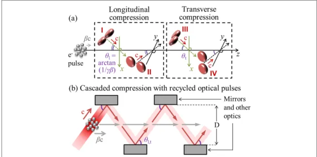
Here, we use the ponderomotive force to compress an electron pulse by subjecting the electron pulse to the intensity minimums of appropriately-oriented Hermite–Gaussian modes, as illustrated in figure1(a). Compression in each Cartesian dimension can be controlled without affecting electron pulse properties in orthogonal dimensions, at the lowest order. Although either pulse I or II suffices for longitudinal compression, using two identical pulses in the configuration shown ensures that any higher-order modulations affecting transverse electron pulse properties do so equally in x and y. Infigure1(a), pulses I and II control compression in z, whereas pulses III and IV control compression in y and x respectively. The stages (and optical pulses) may be arbitrarily ordered and cascaded, as long as inter-particle interactions and dispersion affect the electron pulse negligibly between interactions. Since the ponderomotive force is a nonlinear effect (i.e. not directly
proportional to electricfield), the optical pulses should be sufficiently far apart so that interference between the fields of different pulses does not occur.
The use of an optical pulse’s transverse intensity profile for electron pulse compression has been proposed in [17]. However, the scheme in [17] uses an optical incidence angle normal to the electron path in the lab frame, a sub-optimal configuration for electrons of non-zero speed. In addition, the scheme in [17] uses a Laguerre–
Figure 1. (a) Schematic diagram of three-dimensional electron pulse compression technique using pulsedfirst-order Hermite– Gaussian optical modes, which are portrayed as pairs of shiny red lozenges. Green lines lie in the x–z plane, black lines in the y–z plane. Dotted lines are the beam axes down which the optical pulses propagate. The electron pulse travels at speedv≡βc in the +z-direction,
c being the speed of light in vacuum. γ≡
(
1−β2)
−1 2is the Lorentz factor. (b) Schematic diagram illustrating how a single opticalpulse may be used to implement a succession of compression stages. Lines ending infilled arrowheads sketch the trajectories of optical (red) and electron (gray) pulses, with the arrowheads terminating at the interaction points.
Gaussian‘donut’ mode, which—even for a stationary electron pulse—couples compression in the longitudinal dimension to that in exactly one transverse dimension.
Intuitively, the oblique optical incidence angle of the longitudinal compression stage is motivated by the desire for normal optical incidence in the electron pulse’s rest frame. This implies a lab frame incidence angle of
θ θ γ θ γβ = ″ ″ + =
(
)
c c v arctan sin cos arctan 1 , (1) l l l ⎡ ⎣ ⎢ ⎢ ⎤ ⎦ ⎥ ⎥ ⎛ ⎝ ⎜ ⎞ ⎠ ⎟where the electron pulse propagates in the +z-direction with speedv≡βc(c the speed of light in vacuum), corresponding to Lorentz factor γ≡
(
1−β2)
−1 2. Thefirst equality in (1) expresses the relation between therest frame incidence angleθ ″l andθl. The second equality was made by setting θ ″ =l 90°. We have taken the
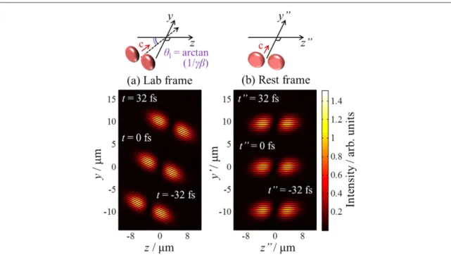
optical group velocity as c, a valid assumption [33] for the paraxial, many-cycle optical pulses we are interested in. The physics behind (1) is illustrated infigure2, which shows how oblique optical incidence in the lab frame corresponds to normal optical incidence in the electron pulse’s rest frame. In the next section, we show mathematically that (1) is optimal in the sense that when it is satisfied, the induced velocity change in the longitudinal direction is not a function of transverse coordinates and not accompanied by transverse phase plane modulations, at the lowest order. Figure3(a) illustrates the physical mechanism of the longitudinal compression scheme: the laser–electron interaction induces a velocity modulation in the electron pulse, which then
compresses as it continues to propagate. The transverse compression scheme works according to the same principles, except that the desired velocity modulation is now along a transverse dimension.
Since the electron pulse is stationary along its transverse dimensions, normal incidence in the rest frame is achieved with any value of θtfor transverse compression. Indeed, we see in section4that the transverse
compression of 30 keV electrons is a relatively weak function of θt. However, the choice of θtcan significantly
affect the longitudinal compression ratio in a three-dimensional compression scheme via higher-order terms of the transverse compression stage, with the best results achieved when θ = °t 0 .
Equation (1) is also the condition for group velocity matching between electron and optical pulses along the axis of electron pulse propagation (i.e.c cosθl=cβ≡v). This observation motivates the cascaded compression
scheme offigure1(b), in which an optical pulse (either pulse I, II, III or IV) is reflected and re-focused by a succession of optical stages, so as to be repeatedly incident upon the electron pulse, allowing the optical pulse to be utilized to its maximum capacity. If (1) is satisfied, the interval between laser–electron coincidences is
γ
=
T D
c , (2)
coin
Figure 2. Intensity profile of pulse II (see figure1(a)) at three instances in time in the (a) lab frame and (b) rest frame of a 30 keV electron pulse. In the lab frame, the temporal pulse and carrier wavefront are obliquely incident at θ =l 70.9°, in accordance with (1), giving rise to normal incidence in the rest frame. Double-primes denote rest frame variables.
3
assuming that the electron pulse is injected along the axis of symmetry of the setup, and that the optical components introduce no delays. To avoid optical interference between successive interactions, D should generally be chosen so thatTcoin≫τis satisfied, τ being the optical pulse duration. With suitable combinations
of optics, one can also implement the design infigure1(b) for any optical incidence angle, or such that a single optical pulse is used to realize several or all of pulses I, II, III and IV, since the four types of pulses essentially differ only in orientation.
3. Theory
In this section, we obtain analytical expressions approximating the ponderomotive potential and net impulse transfer associated with transverse and longitudinal compression by pulsed Hermite–GaussianTEMmnmodes
of arbitrary order. We show mathematically that when (1) is satisfied, the induced velocity change for
longitudinal compression is not a function of transverse coordinates and not accompanied by transverse phase plane modulations, at the lowest order. Although we focus on charged particles, our treatment may be extended to any particle with non-zero polarizability in the Rayleigh regime (particle size much smaller than
electromagnetic wavelength) by the simple replacement of a constant factor. A charged particle in an electromagnetic wave experiences a force [24,25]
⃗ =− + …
F Up , (3)
where the ponderomotive potentialUpis
ω ≡ ⃗ U q m E 4 a , (4) p 2 0 2 2
and q and m0are respectively the particle’s charge and rest mass. The particle sees the electric field
⃗ =
(
⃗ ω +)
E E ea i t c.c. 2, where ⃗Eavaries slowly in time compared to the carrier factor and ≡i −1 . The ellipsis
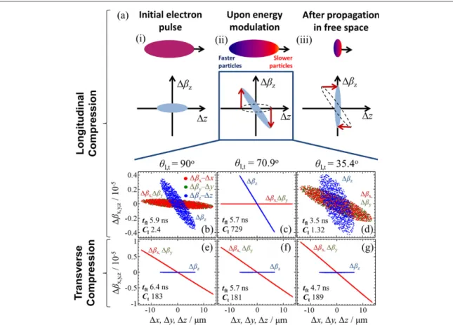
Figure 3. (a) Physical mechanism of the longitudinal compression scheme: (i) the initial electron pulse has afinite spread in momentum and position; (ii) the laser–electron interaction accelerates the back electrons and decelerates the front electrons; (iii) as the pulse propagates, the back electrons catch up with the front electrons, leading to electron pulse compression. Δ ≡z z− z
denotes the particles’ displacement from the bunch centroid along the z-dimension (and so on for the other variables). Phase plane distributions of the 30 keV electron pulse immediately after the longitudinal compression stage are shown for optical incidence angles (b)θ =l 90°, (c) θl=arctan(1γβ)=70.9°, and (d) θ =l 35.4°. Phase plane distributions of the electron pulse immediately after the
transverse compression stage are shown for optical incidence angles (e)θ =t 90°, (f)θ =t 70.9°and (g)θ =t 35.4°. Focal timestfl,ft
in (3) hides terms proportional toe±iωtore±i2ωt. Equation (3) was derived from the Newton–Lorentz equation
in the rest frame of the initial particle. As such, the notion that a particle experiences a force proportional to the gradient of electromagnetic intensity is valid in the rest frame of the particle, and not necessarily in a frame where the particle moves with any substantial velocity. The net momentum imparted to a particle by the passage of a many-cycle pulse is then
∫
∫
△ ⃗ =p F t⃗d = − U tpd . (5)
Physically, the electricfield causes the charged particle to oscillate about its initial position, generating an effective dipole that is subject to the same radiation pressure forces [34] experienced by dielectric particles in optical tweezers [26]. In fact, replacingq m0ω2by α 2 turns (4) into the ponderomotive potential of a particle in
the Rayleigh regime, where the particle’s polarizationP⃗ =αE . The results in this paper thus also apply to⃗
polarizable particles.
A paraxial, many-cycle electromagnetic pulse can be modeled using the vector potential ansatz
ξ ξ ⃗ = ⃗ ψ A Re A˜ ei g , (6) 0 ⎧ ⎨ ⎩ ⎛ ⎝ ⎜ ⎞ ⎠ ⎟⎫⎬ ⎭
where each component ofA˜⃗is a solution of the paraxial wave equation [35], g ( · ) a real even function describing the pulse shape such thatlimξ →∞g( )ξ →0, ξ0a constant associated with pulse duration, ξ≡ωt −k z( −zi)
and ψ≡ξ+ψ0, with zithe pulse’s initial position (at t = 0) and ψ0a phase constant. x, y and z are Cartesian
coordinates.A˜⃗is a slowly-varying function of only spatial coordinates such that∂xA˜ ,⃗ ∂ ⃗ =yA˜ O(ϵd)and
ϵ
∂zA˜⃗ =O
( )
d2 , where the beam divergence angle ϵ ≪ 1d . To ensure that the particle bunch interacts with theelectromagnetic pulse only when the bunch is close to the electromagnetic beam axis (and hence the center of the ponderomotive potential well), we use pulses such that ϵd≪ξ0−1≪1. The electromagneticfields are obtained via the identities [36]
∫
⃗ = × ⃗ ⃗ = ⃗ − ∂ ⃗ ∂ B A E c A t A t · d , (7) 2in which we have applied the Lorenz gauge.
Consider a non-zeroθ (θ= θtorθl) and a particle propagating in the +z direction with speed∣ ⃗ ∣ ≡v βc. We
henceforth denote all variables in the native frame of the electromagnetic pulse with prime superscripts, so the pulse propagates in the + ′z direction, and all variables in the particle’s rest frame with double-prime
superscripts. Non-primed variables x y z t, , , are lab frame variables, defined in accordance with figure1(a). Note that in the rest frame,ω in (4) should be replaced by the Doppler-shifted frequency ω″ ≡ωγ(1−βcos ).θ
Applying the appropriate rotation and Lorentz transformation operators to (6) and (7), we obtain the ponderomotive potential in the rest frame as
ϵ ξ β ″ =
(
′ + ′)
+ +( )
− + U q m A A g 4 ˜ ˜ 1 O( ) O O( ) , (8) x y p 2 0 2 2 2 d 01 ⎡ ⎣ ⎤⎦a result that applies for generalA˜⃗satisfying the paraxial wave equation, assuming thatA˜z′is on the order of the transverse components or less.
For the linearly-polarized Hermite–GaussianTEMmnmode,
ρ ⃗′ ≡ ′ ′ − ′ ′ ′ ′ ′ ′ ′ ′ +
(
) (
)
(
)
A A f f H f x H f y f f ˜ xˆ exp ˜ ˜ * , (9) m n 0 2 m n 2 ⎛ ⎝ ⎜⎜ ⎞⎠⎟⎟where A0is a normalization constant, ′ ≡f i
(
i+ ′z z0)
, ′ ≡x˜ 2x w′ 0, ′ ≡y˜ 2y w′ 0,z0≡ πw02λis theRayleigh range, w0is the beam waist radius, ρ′ ≡ x′ + ′2 y2 w0, and H ( · )m is the Hermite polynomial of
order m (H ( )0 x = 1,H x1( )=2xetc), withm n, ∈ 0(the set of natural numbers including 0). The beam
divergence angle is ϵ ≡d 2 (kw0). From (6) and (7), the peak power P transported in the propagation direction is
∬
ω ϵ π≡ ′ ′ ′ ≈ + −
P S d dx y A c w 2n m n m! !, (10)
z0 2 02 0 02 1
where ′Sz0denotes the z-directed Poynting vector ′ ≡Sz E⃗′ × ⃗′H · ˆz′evaluated at the pulse peak, focal plane and carrier amplitude. ϵ0is the permittivity of free space. The energy U of a single pulse is related to its peak power as
5
∭
∫
ξξ ξω ≡ ′ ′= ′ ′ ′ ≈ ′ ′ U S d d dx y t P g 2 d . (11) z z 0 2 0 ⎛ ⎝ ⎜ ⎞ ⎠ ⎟ ⎛⎝⎜ ⎞⎠⎟Longitudinal compression is achieved with the TEMmnmode when m is odd and n is even. In that case
∫
ξξ ξω ξξ ξ ϵ β ″ = ′ ′ ′ ′ × + + + + + − −( )
(
)
U m K g x g n m 2 d 1 O O ( 1) O( ) , (12) pl 0 l 2 0 1 2 2 0 01 d2 ⎡ ⎣ ⎢ ⎛ ⎝ ⎜ ⎞ ⎠ ⎟ ⎛⎝⎜ ⎞⎠⎟⎤ ⎦ ⎥ ⎛ ⎝ ⎜ ⎞ ⎠ ⎟ ⎡ ⎣ ⎤⎦ where λ π ϵ ≡ − + − K q m c U w m n m n ! ! 2m n [( 1) 2] ! ( 2)! , (13) l 2 2 3 02 0 3 04 2 2 2and we have applied Taylor expansions about the origin in (8) to obtain (12). The net impulse in the rest frame is then
∫
γ β θ Δ θΔ γ β θ θ β θ γ ξ ϵ β △ ⃗ ″ = − ″ ″ ″ = − ″ + ″ − − − × +( )
− +(
+ +)
+ p U t m K x z x z n m d ( cos ) sin (1 cos ) ˆ (cos ) ˆ sin 1 O O ( 1) O( ) , (14) l p 0 l 2 3 01 d2 ⎡⎣ ⎤⎦ ⎡ ⎣ ⎢ ⎤⎦⎥ ⎡ ⎣ ⎤⎦where the particle’s rest frame displacement from the bunch centroid is Δ
(
x″,Δy″,Δz″)
, which we assume does not change significantly during the interaction. To eliminate the x-directed modulation and the Δ ″x -dependenceof the z-directed modulation in the lowest-order term, we must chooseθ such thatcosθ=β, a condition equivalent to (1). The lab-frame velocity change is then
Δ ξ ϵ β
△ ⃗ = −vl zK zˆ l ⎣⎡1+O
( )
0−1 +O ((
n+m+1) d2)
+O( ) ,⎦⎤ (15) where the particle’s lab frame displacement from the bunch centroid is Δ Δ Δ( x, y, z). The longitudinal impulse in the lab frame follows from the relation△ ⃗ =pl m0γ3△ ⃗ +vl O(
△vl2)
. The linear dependence in thelowest-order term of (15) corresponds to a parabolic potential profile. In the absence of space–charge and momentum
spread, a particle pulse would be compressed by a perfectly parabolic potential to a zero extent.
Transverse compression is achieved with the TEMmnmode when m is even and n is odd. In this case,
∫
ξξ ξξ ξ ϵ β ″ = ′ ′ ′ ′ × + + + + + − −( )
(
)
U m K g t y g n m 2 d 1 O O ( 1) O( ) , (16) pt 0 t 2 0 1 2 2 0 01 d2 ⎡ ⎣ ⎢ ⎛ ⎝ ⎜ ⎞ ⎠ ⎟ ⎤ ⎦ ⎥ ⎛ ⎝ ⎜ ⎞ ⎠ ⎟ ⎡ ⎣ ⎤⎦ where λ π ϵ ≡ − + − K q m c U w m n n m ! ! 2m n [( 1) 2] ! ( 2)! . (17) t 2 2 3 02 0 3 04 2 2 2The net transverse impulse imparted by the passage of a single pulse in the rest frame is
γ β θ Δ ξ ϵ β △ ⃗ ″ = − − ″ × +
( )
− +(
+ +)
+ p m K y y n m 1 (1 cos ) ˆ 1 O O ( 1) O( ) , (18) t 0 t 01 d2 ⎡ ⎣ ⎤⎦corresponding to a net lab-frame velocity change of
γ β θ Δ ξ ϵ β △ ⃗ = − − × +
( )
− +(
+ +)
+ v yK y n m ˆ 1 (1 cos ) 1 O O ( 1) O( ) . (19) t t 2 01 d2 ⎡ ⎣ ⎤⎦Asθ approaches0°, the velocity change becomes larger, a result of improved group velocity matching along the optical beam axis. The transverse impulse in the lab frame follows from the relation
γ
△ ⃗ =pt m0 △ ⃗ +vt O
(
△vt2)
. Several noteworthy features of the pulse compression scheme are evident from(13), (15), (17) and (19):
1. At the lowest order, net velocity change is independent of pulse duration parameter ξ0and pulse shape g.
2. A trade-off between the size of the parabolic potential region and the strength of the compression exists in two ways: through the laser waist radius w0, and through the choice of m and n. One solution to achieving a
large parabolic potential region and a large △v for a given total optical energy may lie in the superposition of higher-order Hermite–Gaussian modes, as proposed in [37] in the context of atomic beam imaging.
3. That△ ∝v λ2(as expected of a ponderomotive force scheme [25]) suggests that greater net impulse may be
achieved via longer-wavelength sources. Note, however, that increasing the wavelength increases the pulse duration for the same number of temporal cycles, which may weaken the assumption that the particle’s position relative to the intensity well does not change significantly during the interaction.
The focal time (the time of maximal compression) of a particle pulse with a velocity chirp can be estimated with the formula
= △ t r v , (20) f 0 T
wherevT≡ △ +v v0.△r0and v0refer respectively to the half-width of the particle pulse and the velocity of a
particle at the pulse’s edge, along the dimension of compression and immediately before the interaction. △v is the velocity change induced in the particle at the pulse’s edge as a result of the interaction.
4. Numerical simulations
To numerically model the laser–electron interaction, we solve the exact Newton–Lorentz equation using an adaptive-stepfifth-order Runge–Kutta algorithm [38]. The coordinates of each particle are assigned in a quasi-random fashion using Halton sequences [38]. For the laser pulses, we employfirst-order Hermite–Gaussian modes that are exact (i.e. non-paraxial) solutions of Maxwell’s equations in free space. We readily obtain the fields of a TEM10mode with a Poisson spectrum by using the Hertz vector potential
Π⃗ = ∂ Π ∂ ⃗ x (21) 10 00 in the relations [39] Π ⃗ = ∂ ∂ × ⃗
{
}
B c t Re 1 , 2 10 Π ⃗ ={
× × ⃗}
E Re 10 . (22)The vector potential corresponding to a fundamental Gaussian mode is [40,41]
Π⃗ = Π ′ + − − − − − −
(
)
R f f xˆ 1 s s , (23) 00 0 1 1 wheref± =1− (i )s(
ωt ±kR′ +ika)
, ′ =R ⎡⎣x2+y2+(z+ i )a2⎤⎦ ,andΠ1 20is a complex constant. The
degree of focusing and the pulse duration are controlled through parameters a and s via relations for which good analytical approximations have been derived [40,41]. The non-paraxial Gaussian beam reduces to the phasor of the paraxial Gaussian beam in the paraxial limit [42], so the description (21)–(23) is consistent with (6)–(9).
Unless otherwise specified, all numerical simulations use optical pulses of wavelength λ=0.8 m, waistμ
radiusw0= 180 mμ , and (intensity) full-width-half-maximum (FWHM) pulse duration τ = 50 fs. Each optical
pulse in the longitudinal compression stage has an energy of 17.5 mJ, whereas each pulse in the transverse compression stage has an energy of about 26 mJ. Such specifications fall well within the realm of what is experimentally achievable today. The initial 30 keV electron pulse is a zero-emittance, uniformly-filled ellipsoid of diameter 28μm and length 14 μm, corresponding to a FWHM electron pulse duration of 100 fs. The particles are non-interacting and our simulation results are thus applicable to single-electron pulses. Although actual electron pulses have non-zero emittances that vary depending on factors like the the type of emission
mechanism used [6,43], we use electron pulses with zero initial emittance to perform numerical evaluations of our scheme that are independent of non-idealities in the initial electron pulse.
7
Figures3(b)–(d) depict the numerically computed phase space distributions of electron pulses immediately after the longitudinal compression stage, for various optical incidence anglesθl. The longitudinal magnification Mlis defined asMl≡σz
( )
tfl σz(0), where σz= σz( )t is the standard deviation in z at time t. Here, t = 0 isdefined as the instant captured in figure3(a) (ii) andt =tflthe instant when the longitudinal focus is achieved
(i.e. whenMlis minimized, captured infigure3(a) (iii)). The transverse magnification at the longitudinal focus
isMtl≡ σx
( )
tfl σx(0),where σx=σx( )t is the standard deviation in x at time t. Infigure3(b), we see twoundesirable effects of normal optical incidence in the lab frame, both as analytically predicted in (14): the significant modulation in the transverse phase planes, and the substantial smear in the β△ z− △zphase plane, resulting in a large longitudinal emittance and consequently a weak longitudinal compression factorCl≡Ml−1.
The smeared particle distributions are largely due to walk-off between the center of the ponderomotive potential well and the center of the electron pulse, whereas the presence of transverse modulation is largely due to the oblique optical incidence angle in the rest frame of the electron pulse.
Note that the smearing and transverse modulation exist in spite of the fact that the optical pulse duration
τ = 50 fs is several tens of times smaller than w v0 (w v0( )τ−1≈36≫1), and so nominally satisfies the thin lens
approximation condition prescribed in [17] for normal incidence. This suggests that the thin lens
approximation condition alone is not sufficient for effective longitudinal compression when the kinetic energy is on the order of 30 keV or greater.
As (14) predicts, injecting the optical pulse at an oblique angle according to (1) decouples the longitudinal modulation from the transverse modulation at the lowest order and significantly improves the compression factor from the normal incidence case infigure3(b). This is shown infigure3(c), where we achieve a compression factor ofCl=729, taking the 100 fs electron pulse well into the attosecond regime. Further decreasing the incidence angle, as we do infigure3(d), gives rise again to the substantial smearing of particle distributions in the△βz − △zphase plane, as well as modulations in the transverse phase planes. The sensitivity of the longitudinal compression to the optical incidence angle in the lab frame is further illustrated in figure4(a).
Note that the area occupied in a two-dimensional phase plane is not conserved in the interaction due to inter-dimensional coupling caused by a non-zero magneticfield. This does not violate Liouville’s theorem, which states that the six-dimensional phase space volume is conserved in a Hamiltonian system. Note also that the electron pulse is affected equally in the△βx− △xand△βy − △yphase planes due to our use of both pulses I and II infigure1(a), instead of attempting the longitudinal compression with only one of them.
Figures3(e)–(g) depict the numerically computed phase space distributions of electron pulses immediately
after the transverse compression stage, for various optical incidence angles θt. The transverse magnification is
defined asMt≡σx
( )
tft σx(0),where tftis the time at whichMtis minimal. The longitudinal magnification atthe transverse focus isMlt≡ σz
( )
tft σz(0). Note that because the configuration in figure1(a) subjects the electron pulse to similar treatments in x and y at the lowest order, σybehaves essentially in the same way asσx.The increase in△βx y, (and subsequent decrease in tft) as θtdecreases is as analytically predicted in (19).
Although the transverse compression ratio is a relatively weak function of θt, we see infigure4(b) that the choice
of θtcan significantly affect the longitudinal compression ratio in a three-dimensional compression scheme via
higher-order terms of the transverse compression stage, with maximum longitudinal compression achieved when θ = °t 0 .
Figures4(c) and (d) show the sensitivity of the compression to the displacement of the bunch centroid from the intensity minimum during the interaction. For the cases considered, one should aim to keepθlwithin0.1°of
its optimal value, and the electron bunch centroid within0.01w0of the intensity minimum (values
approximated by considering the half-width-half-maximum of the compression).
Using the simulation parameters offigure3(c) in (15), we obtain △ ≈vl 3.925×10⁻⁶cat △ = −z 6.627
μm (actual value β△ =3.894 ×10−
z 6, relative error 0.80%). For the transverse compression cases, (19) yields
△v ≈3.671×10−c
t 6 at △ = −x 6.945μm in figure3(e) (actual value△βx= 3.644×10⁻⁶, relative error
0.74%) ; △ ≈v 4.113×10−c
t 6 at △ = −x 6.944μm in figure3(f) (actual value△βx =4.081×10⁻⁶, relative
error 0.78 %); and △ ≈v 5.010×10−c
t 6 at △ = −x 6.943μm in figure3(g) (actual value△βx=4.974×10⁻⁶,
relative error 0.72%). These examples demonstrate the accuracy of (15) and (19) in estimating the velocity chirp induced by the interaction.
While the momentum modulations in these examples are small, they are still more than two orders of magnitude greater than the minimum momentum spread required by the Heisenberg uncertainty principle for the electron pulse dimensions considered (Δ Δx px ⩾ 2gives Δγβ ⩾ 1.4×10−
x 8for Δx=14 m).μ
Nevertheless, actually producing an electron bunch with an emittance small enough for the bunch to be affected by such small modulations is currently very challenging (required emittance ϵx∼ Δ Δγβx x< 0.1 nm). In actual
implementations, larger momentum modulations— and hence more realistic emittance requirements—are readily achievable by, for instance, increasing the laser intensity (e.g., by tighter focusing) or introducing more stages in the cascade offigure1(b). For single-electron sources in the tens-of-keV range, emittances as low as 3 nm have been demonstrated [43].
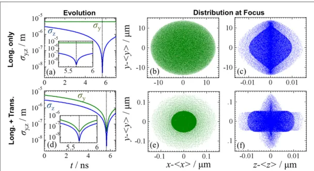
The negative velocity chirp infigure3(c) causes the 30 keV electron pulse to compress longitudinally as it continues propagating after the interaction. Figure5(a) shows the evolution of the electron pulse’s transverse
Figure 4. Sensitivity of compression ratios to (a)θlin a longitudinal compression scheme, (b)θtin a three-dimensional compression
scheme, (c) longitudinal displacement Δzcof the bunch centroid from the intensity minimum in a longitudinal compression scheme,
and (d) transverse displacementΔycof the bunch centroid from the intensity minimum in a transverse compression scheme (along y).
Figure 5. Longitudinal compression of a 30 keV electron pulse from 100 fs to 137 as (longitudinal compression factorCl=729): (a) evolution of standard deviations in y and z, and corresponding spatial distributions at the longitudinal focus (vertical dotted line in (a)) in the (b) y–x and (c) y–z planes. Three-dimensional compression of a 30 keV electron pulse from a duration of 100 fs and a diameter of 28μm to a duration of 137 as and an effective diameter of 0.153 μm ( =Cl 729,Ct=183): (d) evolution of standard
deviations in y and z, and corresponding spatial distributions at the focus (vertical dotted line in (d)) in the (e) y–x and (f) y–z planes.
105particles were used in each simulation. In (a) and (d), the standard deviation in x was omitted as it practically lies over that in y.
9
and longitudinal standard deviations with time. Note that the transverse spread remains practically unchanged from its initial value, even as the electron pulse is compressed from a pulse duration of 100 fs to one of 137 as (Cl=729). The electron pulse distribution at the longitudinal focus, marked by a vertical dotted line in figure5(a), is shown infigures5(b) and (c). The higher-order nonlinear components of the induced velocity chirp prevents the ellipsoid from collapsing into a perfectlyflat pancake.
Figures5(d)–(f) depict the three-dimensional compression of a 30 keV electron pulse from a duration of 100
fs and a diameter of 28μm to a duration of 137 as and a diameter of 0.153 μm ( =Cl 729,Ct=183).θlsatisfies
(1) and θ = °t 0 . Note that simultaneous transverse and longitudinal compression is achieved without affecting the longitudinal compression ratio of the purely-longitudinal-compression scheme infigure5(a).
Figure6depicts the transverse compression of a 30 keV, 1 fs electron pulse from a diameter of 28μm to one of 0.156μm ( =Ct 179). θ = °t 0 here. Infigure6(a), we see that the longitudinal spread remains practically
unchanged from its initial value even as the electron pulse is focused transversely to a very small spot. This demonstrates the ability of the proposed scheme to focus ultrashort electron pulses without inducing temporal resolution-limiting distortions in them.
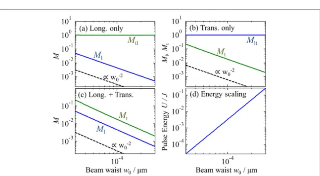
TheUw0−4dependence in (13) and (17) implies that significant energy savings are possible with tighter
focusing. Decreasing the beam waist radius, however, enhances higher-order distortions that limit the maximum achievable compression. Figure7illustrates the tradeoff between compression factor and pulse energy for the value of −
Uw04and the electron pulse used infigures3and5. That the magnification scales asw0−2is
consistent with the fact that the dominant higher-order distortions scale asO
( )
ϵd2 in (15) and (19). Infigure7, UFigure 6. Transverse compression of a 30 keV, 1 fs long electron pulse from a diameter of 28μm to an effective diameter of 0.156 μm (transverse compression factorCt=179): (a) evolution of standard deviations in y and z, and corresponding spatial distributions at the transverse focus (vertical dotted line in (a)) in the (b) y–x and (c) y–z planes.
Figure 7. Scaling of magnification with optical beam waist for the optical and electron pulses of figures3and5: (a) longitudinal compression only, (b) transverse compression only, and (c) three-dimensional compression. (d) plots the scaling of energy U with beam waistw0whenUw0−4is kept constant, from U = 27μJ atw0=30μm to U = 270 mJ atw0=300μm.θlsatisfies (1) andθ = °t 0.
refers to the total energy used in the longitudinal compression stage. Since θ = °t 0 , one may infer from (19) that the energy used for compression in each transverse dimension is typically smaller by a factor of about(1+ β)so that the longitudinal and transverse foci coincide in the three-dimensional compression scheme. Figure7shows that decent compression factors are already attainable with relatively low-energy optical pulses. Infigure7(a), for instance, a longitudinal compression factor of 20 is already achievable with optical pulses of waist radius 30μm and total energy 27 μJ.
Although we have focused on single-electron pulses in this work, the proposed scheme can also be used for multi-electron pulse compression. This is especially (but not only) true when the electron pulse approximates a uniformly-filled ellipsoid or contains a linear velocity chirp. It should be noted, however, that typical multi-electron pulses have much larger diameters—which are on the order of a few hundreds of μm—than the electron pulses considered here, necessitating more energetic optical pulses to achieve the same compression qualities and focal times.
5. Conclusion
We have proposed an all-optical three-dimensional electron pulse compression scheme. The scheme comprises a succession of Hermite–Gaussian optical modes that effectively fashions a three-dimensional optical trap in the electron pulse’s rest frame. Compression in each Cartesian dimension can be controlled without affecting electron pulse properties in orthogonal dimensions, at the lowest order. We showed mathematically that the right choice of optical incidence angle is necessary in longitudinal compression so that the induced velocity change is not a function of transverse coordinates and not accompanied by transverse phase plane modulations, at the lowest order. Although the transverse compression ratio is a relatively weak function of θtfor 30 keV
electrons, the choice of θtcan significantly affect the longitudinal compression ratio in a three-dimensional
compression scheme, with maximum longitudinal compression achieved when θ = °t 0 . We also derived analytical expressions approximating the net velocity change induced in a charged particle by a Hermite– Gaussian optical pulse of arbitrary order and incidence angle. These analytical expressions can be used to estimate the velocity chirp aquired by an electron pulse as a result of the laser–electron interaction.
Finally, using optical pulses that are realizable experimentally, we numerically demonstrated the
longitudinal compression of a 30 keV electron pulse from 100 fs to 137 as (729 times compression), the three-dimensional compression of a 30 keV electron pulse from a duration of 100 fs and a diameter of 28μm to a duration of 137 as (729 times compression) and a diameter of 0.153μm (183 times compression), and the transverse compression of a 1 fs long, 30 keV electron pulse from a diameter of 28μm to one of 0.156 μm (179 times compression). Even larger compression factors are potentially possible with larger beam waists, at the cost of focal time for a given optical pulse energy. Our energy scaling studies show that a compression factor of 20 is already achievable with a 27μJ optical pulse of waist radius 30 μm. The required pulse energies may be lowered further still with the cascade scheme offigure1(b).
The proposed scheme is useful in ultrafast electron imaging for both single- and multi-electron pulse compression, and as a means of focusing ultrashort electron pulses without inducing temporal resolution-limiting distortions in them. Broader applications of the mechanism studied here potentially include
compressing or focusing accelerated protons [44] and neutral atoms [45], enhancing the quantum degeneracy of electron packets [46], creatingflat electron beams [47], and creating ultrashort electron bunches for coherent terahertz emission [48].
Acknowledgments
This work was partially supported by the US Army Research Office Contract No. W911NF-13-D-0001, and the DARPA Young Faculty Award Grant No. D13AP00050. LJW acknowledges support from the Agency for Science, Technology and Research, Singapore. TR acknowledges support from the Alexander von Humboldt Foundation, Germany.
References
[1] Emma P et al 2010 First lasing and operation of an angstrom-wavelength free-electron laser Nat. Photonics4 641–7
[2] Mancuso A P et al 2010 Coherent imaging of biological samples with femtosecond pulses at the free-electron laserflash New J. Phys.12 035003
[3] Sciaini G and Miller R J D 2011 Femtosecond electron diffraction: heralding the era of atomically resolved dynamics Rep. Prog. Phys.74 096101
[4] Zewail A H 2006 4d ultrafast electron diffraction, crystallography, and microscopy Annu. Rev. Phys. Chem.57 65–103
11
[5] Dwyer J R, Hebeisen C T, Ernstorfer R, Harb M, Deyirmenjian V B, Jordan R E and Miller R J D 2006 Femtosecond electron diffraction: making the molecular movie Phil. Trans. R. Soc. A364 741–78
[6] Carbone F, Musumeci P, Luiten O J and Hebert C 2012 A perspective on novel sources of ultrashort electron and x-ray pulses Chem. Phys.392 1–9
[7] Siwick B J, Dwyer J R, Jordan R E and Miller R J D 2002 Ultrafast electron optics: propagation dynamics of femtosecond electron packets J. Appl. Phys.92 1643–8
[8] Michalik A M and Sipe J E 2006 Analytic model of electron pulse propagation in ultrafast electron diffraction experiments J. Appl. Phys. 99 054908
[9] Reed B W 2006 Femtosecond electron pulse propagation for ultrafast electron diffraction J. Appl. Phys.100 034916
[10] Wang Y and Gedik N 2012 Electron pulse compression with a practical reflectron design for ultrafast electron diffraction IEEE J. Sel. Top. Quantum18 140–7
[11] Gao M, Jean-Ruel H, Cooney R R, Stampe J, de Jong M, Harb M, Sciani G, Moriena G and Miller R J D 2012 Full characterization of rf compressed femtosecond electron pulses using ponderomotive scattering Opt. Express20 12048–58
[12] van Oudheusden T, Pasmans P L E M, van der Geer S B, de Loos M J, van der Wiel M J and Luiten O J 2010 Compression of
subrelativistic space–charge-dominated electron bunches for single-shot femtosecond electron diffraction Phys. Rev. Lett.105 264801 [13] Kassier G H, Erasmus N, Haupt K, Boshoff I, Siegmund R, Coelho S M M and Schwoerer H 2012 Photo-triggered pulsed cavity
compressor for bright electron bunches in ultrafast electron diffraction Appl. Phys. B109 249–57
[14] Chatelain R P, Morrison V R, Godbout C and Siwick B J 2012 Ultrafast electron diffraction with radio-frequency compressed electron pulses Appl. Phys. Lett.101 081901
[15] Gliserin A, Apolonski A, Krausz F and Baum P 2012 Compression of single-electron pulses with a microwave cavity New J. Phys.14 073055
[16] Baum P and Zewail A H 2007 Attosecond electron pulses for 4d diffraction and microscopy Proc. Natl Acad. Sci. USA104 18409–14 [17] Hilbert S A, Uiterwaal C, Barwick B, Batelaan H and Zewail A H 2009 Temporal lenses for attosecond and femtosecond electron pulses
Proc. Natl Acad. Sci. USA106 10558–63
[18] Aidelsburger M, Kirchner F O, Krausz F and Baum P 2010 Single-electron pulses for ultrafast diffraction Proc. Natl Acad. Sci. USA107 19714–9
[19] Zewail A H 2010 Four-dimensional electron microscopy Science328 187–93
[20] Veisz L, Kurkin G, Chernov K, Tarnetsky V, Apolonski A, Krausz F and Fill E 2007 Hybrid dc–ac electron gun for fs-electron pulse generation New J. Phys.9 56694
[21] Weninger C and Baum P 2012 Temporal distortions in magnetic lenses Ultramicroscopy113 145–51
[22] Novotny L, Sánchez E J and Xie X S 1998 Near-field optical imaging using metal tips illuminated by higher-order Hermite–Gaussian beams Ultramicroscopy71 21–29
[23] Chu S-C, Chen Y-T, Tsai K-F and Otsuka K 2012 Generation of high-order Hermite–Gaussian modes in end-pumped solid-state lasers for square vortex array laser beam generation Opt. Express20 7128–41
[24] Eberly J H, Javanainen J and Rza̧żewsk K 1991 Above-threshold ionization Phys. Rep.204 331–83
[25] Boot H A H and Harvie R B R-S 1957 Charged particles in a non-uniform radio-frequencyfield Nature180 1187 [26] Ashkin A 1997 Optical trapping and manipulation of neutral particles using lasers Proc. Natl Acad. Sci. USA94 4853–60 [27] Dodin I Y and Fisch N J 2007 Particle manipulation with nonadiabatic ponderomotive forces Phys. Plasmas14 055901
[28] Stupakov G V and Zolotorev M S 2001 Ponderomotive laser acceleration and focusing in vacuum for generation of attosecond electron bunches Phys. Rev. Lett.86 5274–7
[29] Siwick B J, Green A A, Hebeisen C T and Miller R J D 2005 Characterization of ultrashort electron pulses by electron–laser pulse cross correlation Opt. Lett.30 1057–9
[30] Hebeisen C T, Ernstorfer R, Harb M, Dartigalongue T, Jordan R E and Miller R J D 2006 Femtosecond electron pulse characterization using laser ponderomotive scattering Opt. Lett.31 3517–9
[31] Morrison V, Chatelain R P, Godbout C and Siwick B J 2013 Direct optical measurements of the evolving spatio-temporal charge density in ultrashort electron pulses Opt. Express21 29–37
[32] Harb M, Ernstorfer R, Dartigalongue T, Kruglik S G, Hebeisen C T, Sciaini G and Miller R J D 2008 Grating enhanced ponderomotive scattering for visualization and full characterization of femtosecond electron pulses Opt. Express16 3334–41
[33] Esarey E, Sprangle P, Pilloff M and Krall J 1995 Theory and group velocity of ultrashort, tightly focused laser pulses J. Opt. Soc. Am. B12 1695–703
[34] Harada Y and Asakura T 1996 Radiation forces on a dielectric sphere in the Rayleigh scattering regime Opt. Commun.124 529–41 [35] Mandel L and Wolf E 1995 Optical Coherence and Quantum Optics (Cambridge: Cambridge University Press)
[36] Jackson J D 1975 Classical Electrodynamics 2nd edn (New York: Wiley) [37] Steuernagel O 2009 Optical lenses for atomic beams Phys. Rev. A79 013421
[38] Press W H, Teukolsky S A, Vetterling W T and Flannery B P 1992 Numerical Recipes in C 2nd edn (Cambridge: Cambridge University Press)
[39] Sheppard C J R 2000 Polarization of almost-plane waves J. Opt. Soc. Am. A17 335–41
[40] April A 2010 Ultrashort, strongly focused laser pulses in free space Coherence and Ultrashort Pulse Laser Emission ed F J Duarte (Rijeka: InTech)pp 355–82
[41] Wong L J, Kärtner F X and Johnson S G 2014 Improved beam waist formula for ultrashort, tightly focused linearly, radially, and azimuthally polarized laser pulses in free space Opt. Lett.39 1258–61
[42] April A 2008 Nonparaxial elegant Laguerre–Gaussian beams Opt. Lett.33 1392–4
[43] Baum P 2013 On the physics of ultrashort single-electron pulses for time-resolved microscopy and diffraction Chem. Phys.423 55–61 [44] Robson L et al 2007 Scaling of proton acceleration driven by petawatt-laser–plasma interactions Nat. Phys.3 58–62
[45] Eichmann U, Nubbemeyer T, Rottke H and Sandner W 2009 Acceleration of neutral atoms in strong short-pulse laserfields Nature461 1261–4
[46] Spence J C H, Qian W and Silverman M P 1994 Electron source brightness and degeneracy from fresnel fringes infield emission point projection microscopy J. Vac. Sci. Technol. A12 542–7
[47] Zhu J, Piot P, Mihalcea D and Prokop C R 2014 Formation of compressedflat electron beams with high transverse-emittance ratios Phys. Rev. ST Accel. Beams17 084401
[48] Li Y and Kim K-J 2008 Nonrelativistic electron bunch train for coherently enhanced terahertz radiation sources Appl. Phys. Lett.92 014101