Analysis and implementation of the bilayer microfluidic geometry

Analysis and Implementation of the Bilayer

Microfluidic Geometry

by

Niraj K. Inamdar

B.S.E, University of Pennsylvania (2008)

Submitted to the Department of Mechanical Engineering

in partial fulfillment of the requirements for the degree of

Master of Science in Mechanical Engineering

at the

MASSACHUSETTS INSTITUTE OF TECHNOLOGY

MASSACHUSETTS INSTITUTE OF TECHNOLOGY

JUL 2 9 2011

LIBRARIES

ARCHNES

June 2011

@

Niraj K. Inamdar, 2011

Author.

Department of Mechanical Engineering

May 5, 2011

Certified by

Linda G. Griffith

Professor of Mechanical and Biological Engineering

I

.- .

Thesis Supervisor

Certified by

gi

_{Jeffrey T. Borenstein}

Director, Department of Biomedical Engineering, Charles Stark

6)

Draper Laboratory

Thwi S u.rvisor

Accepted by...

David Hardt

Chairman, Committee on Graduate Studies, Department of

2

Analysis and Implementation of the Bilayer Microfluidic

Geometry

by

Niraj K. Inamdar

Submitted to the Department of Mechanical Engineering on May 5, 2011, in partial fulfillment of the

requirements for the degree of

Master of Science in Mechanical Engineering

Abstract

Microfluidic devices form an important class of analytical platforms that have found wide use in the biomedical sciences. In particular, they have been used in cell culture systems, where they are used to monitor cell behavior in various environments. One challenge that has emerged, however, is the ability for a microfluidic device to uniformly deliver soluble factors to a given culture of cells without subjecting the cells to hydrodynamic shear stresses that could potentially alter their behavior in an unpredictable or undesirable way. This is especially true for a number of cell types, and striking a balance between solute transport and shear stress remains the subject of active research. In this thesis, we will consider a membrane bilayer device configuration in which the transport of a solute to a cell population is achieved by flowing solute through a proximate channel separated from the culture channel by a membrane and seek to characterize some of its hydrodynamic and transport characteristics. It will be shown analytically that this configuration affords greater flexibility over a more traditional single-channel setup, in terms of control over solute transport and applied shear. We will also discuss some topics related to the flow fields within such devices, as well as the fabrication and implementation of the bilayer microfluidic device in an experimental setting.

Thesis Supervisor: Linda G. Griffith

Title: Professor of Mechanical and Biological Engineering

Thesis Supervisor: Jeffrey T. Borenstein

Title: Director, Department of Biomedical Engineering, Charles Stark Draper Laboratory

Acknowledgements

I would like to thank MIT and my advisor, Professor Linda Griffith, for providing me with the opportunity and the financial support to study here. I would also like to thank Draper Laboratory, its Educational Office, and the technical staff there for providing me with many resources and a great deal of technical assis-tance during my nearly two years as a Draper Fellow. In particular, I'd like to thank my advisor at Draper, Dr. Jeff Borenstein, who became as much a friend as an advisor, and who helped make my experience here very enjoyable.

I would also like to thank my sister for her friendship, and Blythe Boyd for the

kindness, support, and love she has shown me over the last few years. Finally, I would like to thank my dad, who has encouraged me and supported all my inter-ests (both technical and non-technical) throughout my life. He is-and always will be-my best friend.

Some of the content of this thesis has appeared in references [1], [2], and [3].

The project described was supported by Award Number RO1EB010246 from the National Institute of Biomedical Imaging and Bioengineering. The content is

solely the responsibility of the author and does not necessarily represent the official views of the National Institute of Biomedical Imaging & Bioengineering

or the National Institutes of Health. The author hereby grants to MIT and Draper Laboratory permission to reproduce and to distribute publicly paper and

Contents

1 Introduction 13

1.1 Microfluidics... ... .. ... .. .. .. . .. 13

1.2 Motivation and Scope of Thesis... . . . . . . . .. 14

2 Analytical Investigation: Molecular Transport 19 2.1 Introduction . . . . 19

2.2 Single Channel Case . . . . 21

2.2.1 Equations of transport . . . . 21

2.2.2 Characteristic Time and Length Scales . . . . 21

2.2.3 Single Channel Equation of Transport: Continued. . . . . . 24

2.2.4 Solution . . . . 25

2.3 Monoculture Bilayer Case . . . . 29

2.3.1 Equations of Transport . . . . 29

2.3.2 Solution . . . . 31

2.3.3 Application of boundary conditions to the solution . . . . . 33

2.3.4 Average Outlet Concentration . . . . 35

2.4 Coculture Bilayer Case . . . . 36

2.4.1 Solution . . . . 37

2.5 Param eters . . . . 38

2.6 R esults . . . . 41

2.6.1 Single Channel and Monoculture Bilayer . . . . 41

2.6.2 Coculture Bilayer . . . . 44

2.7 D iscussion . . . . 45

3 Analytical Investigation: Hydrodynamics 59 3.1 Introduction... . . . . . .. 59

3.2 Disturbances in the y-direction Flow Field.... . . . .. 60

3.3 Two-Dimensional Channel... ... . . . . . . . . . .. 64

3.4 Perturbed flow field in the bilayer . . . . 68

4 Implementation of a Bilayer Device

81

4.1 Introduction . . . . 81

4.2 Overview: Materials, Design and Fabrication . . . . 82

4.2.1 M aterials . . . . 84

4.3 Implementation of Design . . . . 86

4.4 Some Initial Experiments to Determine Membrane Parameters . . . . 90

4.4.1 Determining Dmembrane . . . .. 90

4.4.2 On the experiment for determining o . . . .. 92

4.5 Culturing hTERT MSCs in the Device . . . . 96

5 Conclusions

101

5.1.1 Short-Term Goals . . . 102

5.1.2 Long-Term Goals . . . 103

A Some Theorems for Partial Differential Equations

107

A.2 Possible solutions to Laplace's equations with certain boundary con-d ition s . . . 110

B Fabrication Protocol for Silicon Wafer

111

C Cell Culture Protocols for hTERT MSCs

113

C.2 Protocol Used for Splitting hTERT MSCs... . . . . .. 114

C.3 Protocol Used for Feeding hTERT MSCs . . . 115

D Backflow in Y-Channel

117

E Data from measurements to determine

o-

119

List of Figures

1-1 Schematic of single channel and bilayer microfluidic device. . . . . . 16

2-1 Cross-sectional geometry and geometrical parameters of single chan-nel and bilayer constructs... . . . . . . . ... 20 2-2 Comparison of concentration at cell surface for single channel and

bilayer cases. . . . . 46

2-3 Concentration fields for single channel and bilayer geometries. . . . 47 2-4 Concentration at cell surface as a function of x for Cases 1, 2, and

3: B aseline. . . . . 48

2-5 Concentration at cell surface as a function of x for cases 1, 2, and

3: Increased flow rate in upper chamber.... . . . . . . . 49

2-6 Concentration at cell surface for varying Co. . . . . 50 2-7 Average outlet concentration for single channel case for varying flow

rates... ... ... ... 51

2-8 Average outlet concentrations for monoculture bilayer flow channel and cell compartment for varying F: Case 1. . . . . 51 2-9 Average outlet concentrations for monoculture bilayer flow channel

and cell compartment for varying F: Case 2. . . . . 52

2-10 Average outlet concentrations for monoculture bilayer flow channel and cell compartment for varying F: Case 3. . . . . 52

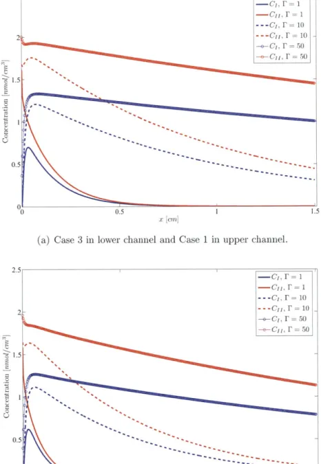
2-11 Coculture concentration at cell surface for varying F: Case 1 lower channel and Cases 1 and 3 in the upper channel. . . . . 53

2-12 Coculture concentration at cell surface for varying F: Case 2 lower channel and Cases 2 and 3 in the upper channel. . . . . 54

2-13 Coculture concentration at cell surface for varying F: Case 3 lower

channel and Cases 1 and 3 in the upper channel. . . . . 55

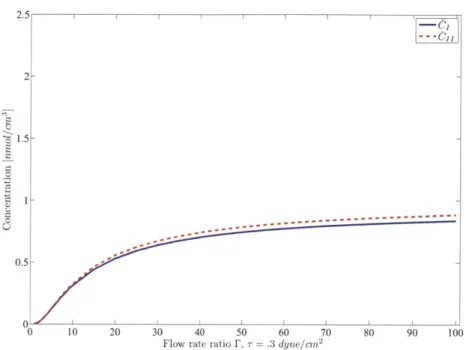
2-14 Average outlet concentration for coculture bilayer configuration with varying F: Case 1 in upper channel and Case 3 in lower channel. . . 56 2-15 Average outlet concentration for coculture bilayer configuration with

varying F: Case 2 in upper channel and Case 2 in lower channel. . . 56 2-16 Average outlet concentration for coculture bilayer configuration with

2-17 Average outlet concentration for coculture bilayer configuration with

varying F: Case 3 in upper channel and Case 3 in lower channel. . . 57

2-18 Reduction of the depletion zone in the bilayer construct. . . . . 58

3-1 Overall device configuration with tubing. . . . . 63

3-2 Characteristic disturbance length 6 as a function of tube length ltbe,2 for various diameters dtube . . . . 65

3-3 Percentage of channel width that can be approximated by two-dimensional flow field within error E for various channel aspect ratios. 68 4-3 Channel cross-section measured by profilometer.. . . . . . . . . 89

4-4 Soft lithography fabrication process for microfluidic device. . . . . . 89

4-5 Sample devices made from PDMS. . . . . 90

4-6 Outlet concentration in terms of percent saturation measured as a function of tim e . . . . 93

4-7 Experimental setup... . . . . . . . .. 93

4-8 Experimental data for hL... . . . . . .. 97

4-9 Cells in microfluidic device after one day... . . . . .. 98

4-10 Cells in microfluidic device after two days... . . . .. 98

4-11 Cells in microfluidic device after two days. . . . . 99

4-12 Cells in microfluidic device after two days... . . . .. 99

List of Tables

2.1 Parameters for channel.. . . . . 23

2.2 Characteristic times and development length for

Q

2.3 Coefficients of expansion for ai = 0. . . . . 26

2.4 Coefficients of expansion for ao = 0. . . . . 27

2.5 Baseline parameters used. . . . . 40

2.6 Combinations of parameters for various cases. . . . . 40

3.1 Parameters for membranes with pore diameters dpore = .8 pm and 8 p m . . . . . 64

4.1 Parameters for membrane experiment.. . . . . . . . . . 96

Chapter 1

Introduction

1.1

Microfluidics

Microfluidic systems have emerged as revolutionary new platform technologies for a range of applications, from consumer products such as inkjet printer cartridges to lab-on-a-chip diagnostic systems. The development of microfluidic-based tech-nologies over the past two decades has spawned advances in fields ranging from laboratory diagnostics to consumer devices, spurred by emerging requirements in molecular analysis, biodefense and microelectronics. Microfluidics have also found wide application in the field of bioengineering as platforms upon which tissue for a wide range of biological systems can be cultured and engineered for comprehensive and high-throughput analysis, and implantation and organ replacement. Microflu-idic devices have given researchers the ability to develop more physiologically rel-evant assays by allowing for the concurrent study of mechanical and biochemical effects on tissue culture. Moreover, in light of shortages of organs available for transplantation, microfluidic devices have been used to develop architectures for implantable tissue for therapeutic purposes.

flu-ids within geometries with characteristic length dimensions on the order of ten to a hundred microns [4]. Microfluidics have become indispensable tools partly due to their size, since they can be made to accommodate anywhere between millions of cells to single cells. Moreover, they have also found favor with bioengineers and clinicians due to the presence of fluid flow, an important physiological condition which is naturally not present within static culture dishes. Microfluidic devices are relatively fast and easy to design and fabricate, and the most commonly used fabrication processes exploit techniques from the microelectronics and other in-dustries and permit for the fast and easy fabrication of a large number of devices. These factors combine to make microfluidics an attractive technology upon which tissue engineering and related research can be conducted.

From an experimental point of view, a notable advantage of microfluidic cell culture is the potential to control concentrations of nutrients, growth factors, and other soluble regulatory molecules within the microfluidic environment; this stands in direct contrast to static cell culture dishes that are the norm. However, while microfluidic devices have developed into powerful, comprehensive experimental tools, there still remain several challenges if a microfluidic device is to be fully modular and capable of isolating important biochemical and mechanical factors in the in vitro environment.

1.2

Motivation and Scope of Thesis

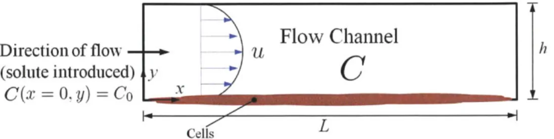
In a typical microfluidic culture device, fluid is flowed directly over cells cultured in a single channel [Figure 1-1(a)], and as a consequence, fluidic shear is imparted directly on the cells. However, it is known that for certain cell types, metabolic ac-tivity, differentiation, and proliferation are sensitive to shear stresses [5, 6, 7, 8, 9]. It is possible, then, in the course of an assay, that cellular responses that are

mea-sured are altered by the presence of shear. Moreover, delivering the same amount of solute to all the cells cultured may become a challenge, for in a typical config-uration, in which cells are cultured and medium flowed through a single channel configuration, equitable delivery may only occur by increasing the flow rate and consequently, shear. Hence, it is also preferable experimentally to deliver a con-trolled quantity of solute to the cell population while at the same time having independent control over the imparted shear. We may attempt, then, to seek an alternative device configuration. Some have already been analyzed in the litera-ture, and utilize unique biologically-inspired [8] or grooved geometries [10] to shield cells from shear. Instead, we will analyze the bilayer construct [11, 12], which af-fords itself to a much more straightforward analysis and offers greater simplicity in the way of fabrication and operation.

A bilayer device [Figure 1-1(b)] is one in which the cell culture region (the cell

compartment) is separated from a flow channel by a semipermeable membrane.

This allows for the possibility of decoupling solute transport to the cell culture and the fluidic shear imparted to the culture. In principle, the medium flow rate in the upper channel is set at a relatively high rate while modulation of the membrane transport characteristics and the flow rate in the flow channel then enables independent control of solute transport.

In this thesis, we will consider the application of the bilayer construct to a culture of mesenchymal stem cells (MSCs). A stem cell culture has been cho-sen for the model analysis for several reasons. First, stem cells have been the focus of a great deal of research in recent years due to their pluripotent nature, and their consequent potential for therapeutic uses in regenerative medicine [13]. Thus, developing an experimental platform for their study has considerable prac-tical interest. In terms of physiological variables, shear stresses have been shown to regulate activation of signaling pathways, gene expression, proliferation, and

os-Direction of flow

(solute introduced)

Cells

Direction of flow

(solute introduced)

Solute transport across membrane

Cell Compartment

Solute consumption by cells

Outlet flow

Porous

membrane

Outlet flow

Cells

Figure 1-1: Schematic of (a) single channel and (b) bilayer microfluidic device

operating in a monoculture mode. In the single channel device configuration,

medium flow is directly over culture. Solute, which is introduced at the left hand

side of the channel, is convected forward and diffuses downwards towards the

culture. In the bilayer configuration, medium flow is primarily in the upper flow

channel, while the flow in the lower cell compartment is modulated depending

on the shear requirements of the culture experiment. Solute is introduced at the

left hand side of the flow channel, wherein it is convected forward while diffusing

downwards and across the membrane; once solute enters the cell compartment, it

continues to diffuse downwards towards the cell culture, where it is consumed by

the cells.

Flow Channel

Solute consumption by cells

_{Outlet flow}

Flow Channel

teogenesis in MSCs [9, 5, 6, 14, 15]. Moreover, in response to low oxygen tensions (such as might be found during embryonic development [16], or in the bone mar-row), MSCs upregulate hypoxia-induced factors that then control cell behaviors such as proliferation and differentiation into osteoblasts or chondrocytes [17, 18]. As such, stem cells lend themselves naturally to the study and validation in a bilayer microfluidic device.

The content of this thesis will be divided into three chapters, corresponding to Chapters 2, 3, and 4. In Chapter 2, we will apply a simple mathematical model describing the transport of oxygen within a bilayer device to a culture of mesenchy-mal stem cells (MSCs). In Chapter 3, we will touch upon some aspects of fluid flow within the bilayer construct and discuss the possibility of controlling trans-membrane fluid flow that will be present should flow rates in the flow channel and cell compartment be different. We will conclude in Chapter 4 by discussing various considerations that go into the fabrication of a bilayer device and by demonstrating some preliminary experiments on a device that was actually fabricated. We note that in this thesis, due to the constraint of time, we only touch upon each of the aforementioned aspects. It is envisioned that this work will lay the foundation for

a more comprehensive study of the characteristics of the bilayer geometry under a variety of biologically relevant conditions. Finally, it is hoped that this platform can be applied towards gaining a greater understanding of the differentiation and proliferation of stem cells under a greater variety of mechanical and biochemical

Chapter 2

Analytical Investigation:

Molecular Transport

2.1

Introduction

In this chapter, we will analytically investigate the transport characteristics of oxygen in a bilayer construct cultured with mesenchymal stem cells, and analyze some aspects of the bilayer's transport properties. The investigation will proceed as follows: We will first consider the general equation of transport, then reduce it using scaling arguments to an analytically tractable form. Subsequently, we will consider the single channel case, in which cells are cultured at the bottom of the flow channel, and derive the general solution to the transport equation. We will then extend the general solution to the monoculture bilayer case (that is, the case in which cells are cultured solely in the cell compartment) by applying the appropriate boundary conditions, and finally, do the same for the coculture bilayer case, in which cells are cultured in both the flow channel and the cell compartment. The last case may be of interest in future studies in which different types of cells are cultured in one device and we are interested in (say) intercellular

communication between the populations. We will close by presenting the results of some calculations for each case and by comparing and discussing their implications.

Direction of flow

-(solute introduced)

C(x

=

0, y) =

Co

(a) Single channel cross-sectional geometry with relevant dimensions.

-,.

Flow Channel

Direction of flow

-(solute introduced) y _II

C1(x = 0, y) = CO

Membrane

Small Cell Compartment

Direction of flow

--

perfusion

C

(x = 0, y) = 0

y

x

ILt

Cells

(b) Bilayer cross-sectional geometry with relevant dimensions.

Figure 2-1: Cross-sectional geometry and geometrical parameters of (a) single channel and (b) monoculture bilayer device constructs. It is assumed that the channel width w (into the page) is much greater than the channel heights, h, hr, and h11, for both cases.

--

Flow Channel

|-

L

2.2

Single Channel Case

2.2.1

Equations of transport

Generally, in two dimensions, the concentration of a given solute is governed by the transport equation:

ac

ac

ac

a2C

8a

_C

+ U

+v-

= D

+

-

(2.1)

at

ax

ay

D

ax

(

u and v are the velocities of the fluid in the horizontal (x) direction and in the

vertical (y) direction, respectively. For a long, rectangular channel in which flow is sufficiently developed, we can take v = 0, and moreover, we may assume the configuration has reached steady state, so that

aC/at

take

a

/ax

₌

_{0. Eq. (2.1) will then reduce to}

OC(x, y) _{82C(X, y)}

U

ax

=

D

.

(2.2)

2.2.2

Characteristic Time and Length Scales

We may opt to instead to justify the reduction to Eq. (2.2) on a more quanti-tive basis, rather than on qualitaquanti-tive, dimensional arguments. In considering the dominant terms in the momentum and transport equations, we must consider the time scales characteristic to each physical process. In the momentum equations (i.e., the Navier-Stokes equations), we are interested in knowing how long and far it takes the system to reach a steady state and full development, while in the transport equations, we wish to know, in a given direction, whether transport is diffusion-dominated or convection-dominated.

Momentum Transport

For fluid flux, the characteristic development time, tdev is given by

~ h2

tdev

~"(2.3)

where h is the height of the channel and v is the kinematic viscosity of the medium. For the development length Ldev of the fluid flow (i.e. the length it takes for the boundary layers on all sides of an enclosed channel to meet), numerous correlations exist. One such expression reads

[19]

0.6

Ldev = Dh + 0.056 ReL (2.4)

11 + 0.035 ReLI

where ReL, given by pfluiduoL/p, is the Reynolds number of the flow with respect to the channel length L, uo is the mean velocity of the flow, and Dh is the hydraulic diameter of the channel, given by 2hw/(h

+

Molecular Transport

The two means of molecular transport, diffusion and convection, have characteris-tic time scales, tdff and tconv respectively, given, along the length of the channel,

by

tdiff = L2

/D

teonv

= L/uo

(2.6)

typical as reported in the literature; they are summarized in Table 2.1. Parameter Value h 50 pn [20, 21] w 200 pm [20, 21] Dh 80 pm L 1.5 cm [20, 21] D 3.55 x 10-5 cm2_{/s [22]} Pfluid 1000 kg/m 3

P

V

Table 2.1: Parameters for channel.

For a volumetric flow rate

Q

basis of the maximum allowable shear to which the cell culture may be exposed), we have uo = Q/(hw) = .25mm/s. The resulting characteristic times and lengths

for this

Q

Parameter Value ReL 4.2135 tdev 2.8 ms Ldev 60.7 pm tdif f 63, 380 s teen_ 60 s

Table 2.2: Characteristic times and development length for

Q

Clearly, ico,,

<

become comparable. By Eqs. (2.5) and (2.6), if tdif ~ icon,

hwD

(2.7)

L

For the parameter values given above,

Q

/s

2.2.3

Single Channel Equation of Transport: Continued.

Physically, the transport Eq. (2.2) and the analysis above suggest that transport in the x-direction is convection-driven, while in the y-direction, it is diffusion-driven. We have indicated explicitly the dependence on y of u. More precisely, it takes the well-known form

h2

dp

_(2.8)

(y) =1(dx

_2p

_dx

_.h

_h.

₂

In order to make the transport equation more generally applicable, we will now non-dimensionalize it. First, we let a characteristic fluid velocity O =- (-dp/dx)h2_(8p)-1

_.

Additionally, we let a characteristic concentration be Co and scale x and y against the height of the channel h. Then, Eq. (2.2) becomes, in terms of non-dimensional coordinates and a scaled C,

BC(x, y)

1 8

_{C(x, y)}

4y(1 - y)

(2.9)

By

Peh

y

where Peh is the well-known Peclet number, defined as

uoh/D.

L is the original length of the channel in the x-direction and h the height in the

y-direction, that now x E [0, L/h] and y

E

We may also note that Peh is dependent upon the volumetric flow rate

Q

w of the device, it may be found that

3Q

Peh =

2wD (2.10)

2.2.4

Solution

We will now derive the general solution to this equation before prescribing any relevant boundary conditions. First, let C(x, y) = (x)(y). Inserting this into

Eq. (2.9) and rearranging gives

1 4y(1 - y)('(x)i(y) = I (

Peh (2.11)

so that separating leaves us with

4Peh

(x)

where A2 is some constant.

The left side of Eq. (2.12) is integrated immediately:

((x) = A exp (- x),

(4 Peh

where A is some constant, while the q portion may be rearranged to give

T1 "(y) +

A

_y(1

The solution for 17(y) will be found by method of power series. Since Eq. (2.14) is non-singular over the domain [0, 1], we may assume (y) = E' ayny. Substitut-ing this into Eq. (2.14) and equatSubstitut-ing powers of y yields a recurrence relationship

for the coefficients a, of the expansion: _ 2

an = (- (an-3 - an_4)

n(n - 1)

where ao and ai are to be determined and a2 may be seen to be 0. First, we let

ai = 0; then we may find the coefficients of the expansion a") (factoring out the

common ao) satisfying Eq. (2.14); they are given in Table 2.3.

Table 2.3: Coefficients of expansion for a1 = 0.

Then, we may let ao = 0, so that after factoring out ai, the coefficients for the

expansion anP can be obtained; these are given in Table 2.4. Thus, r/(y) may be completely written as

r/(y)

00 00

= aoE a(0)y"

+

n=O n=o

If we multiply this result by Eq. (2.13), we have the solution to Eq. (2.11). If we ai = 0 (0) Coefficient, an Value a0 1 a(0) a1

0

a(O)

0

Table 2.4: Coefficients of expansion for ao = 0.

do this and divide out by ao, we have a general solution of

C(x, y) A exp -= _{A exp (} n=o 00 ai n-o

any"

where 1/ao has been subsumed into the constant A, ai/ao redefined as a1, and

T(y) redefined as indicated.

Boundary conditions

In a dimensional system, we will suppose that at the left-hand boundary (the line

x = 0), we have a given fixed concentration CO of solute; that is, C(x = 0, y) = Co.

ao = 0 Coefficient, an Value a(l) 0 a0 (1) 1 a4 12 (1) _ 522

afl

0

In our non-dimensional system,

C(x = 0,y)

=

1

At the lower boundary, we will assume Michaelis-Menten kinetics for the consump-tion of the solute by the cells [23]. Therefore, in the dimensional system

D1C

(9y YO

VmaxPcensC(X, y = 0)

Km + C(x, y = 0)

where Vmax is the maximum rate of consumption, Km is the consumption rate at which the expression evaluates to Vmax/2, and pce, is the linear density of the cells. With our assumption of a low-oxygen fluidic environment, we expand the right hand side into a Taylor series:

VmaxPceisC(X, y = 0) Km + C(x, y = 0) C(x, y

= 0)

(C(x,y = 0) )

Then the y boundary condition reads to the first order

D a

C(x y

Vmax Pcen Km

Non-dimensionalizing this gives then

aC

ay

(C(x, y = 0)

Km

where Da -- Vmawxpcsh/(DKm..) is the Damkohler number. We have at the upper boundary a no-flux condition, so that in our non-dimensional system

C

= 0

(2.19)

Oy Y=

Eq. (2.19) gives a characteristic equation in the Aj, which is to be solved. Then

the complete solution to Eq. (2.11) in non-dimensional form is given by

Cx,

y)

Ai exp

i=O (-4 Peh )

where each i' is distinguished according to Ai and Ai is given by

A =o r/(y)y(1 - y)dy

f

Ir/77(y)

y (1 - y) dy

an elementary result in accordance with Sturm-Liouville theory, which may be de-rived by demonstrating the self-adjointness of Eq. (2.11) with the given boundary conditions. In dimensional form, the solution may be writen

00

AD X

C(x, y) = Co

A

exp

- Jr(y/h)

(2.20)

4uo

2.3

Monoculture Bilayer Case

2.3.1

Equations of Transport

We now consider the solution to the transport equation in the monoculture bilayer case. The region of interest is taken as a whole to be the union of two rectangular regions, both of length L. The upper region is denoted QHr, and is characterized

of hr. In applying the non-dimensionalization scheme to Qrr and Qr, we use as the reference height hr. Denote the concentrations of interest to be C1, and C,

for the upper and lower channels, respectively. Assuming no transmembrane

fluid

flux,

4y

y

Y

B r(x, y)

0 I

x E [0 L/hr]

and

- Cr (x, y)

4y(1 - y). O (,Y

E

y

xCG [0, L/h

]

1 a

_C

,(X,y)

#]-1

C

(x,

y)

and y E [0, 1], [0, L/h]

[0, 1]

Q,

where

#3

hrr/hi,

uo,irhr/Dii,

uo,

(-dp1/d)hir(8

1)-

and uo,r equal to (-dp/d)h2(8

u)->.

Again, in terms of

flow rates

Qr

3QI

2wD

2/iwDj

2.3.2

Solution

The general methodology used in Section 2.2.4 may be used to derive the general solutions for Eqs. (2.21) and (2.22). The general solution to Eq. (2.22) is then

= A, exp( = A exp(-4 Pe,

X)

a(O

yn

+

4Per

where the coefficients a() and a l)are defined as in Tables 2.3 and 2.4.

Eq. (2.21), the presence of the factor of

#

Cr (x, y)

= A,,

exp

A,

+a,,,,

a~3

The coefficients a and aW0 are found nearly as they were in the previous section, with the difference being that the coefficients must all be divided by a factor of

#2;

In the x-direction, we will again have prescribed conditions; that is,

C1(x = 0, y)

C (x=

0,

y)

= Co

OC

I: a(O)

-In our non-dimensional system,

C1

(X = 0, y)

Ci(x = 0, y)

(2.27) (2.28)

Let us assume that the media in both channels are the same; then D, = D-r = D. In Q1, we have the following y boundary conditions:

D CI

DDCI

C1(z, y = 0)

=

k[Cj

(x,y=

0)-C1(x,y=h)];

k may be seen to be the diffusion coefficient of the membrane divided by the thickness of the membrane. Again, non-dimensionally:

= DaCi(x,y

₌

DKm

= Sh [C

r(x,

y =

0)

-

C(x,

y

1)],

Sh -

(kh

/D)

In

QHr,

y = 0 follows from the above, so that non-dimensionally,

By-ac

Oy

_,O

OCI

dy

Y_1

y

Dy

Y=

2.3.3

Application of boundary conditions to the solution

For QGj, the no-flux boundary condition on the top surface requires

Oc'

1

(9y

Cri (x,

y)

= A,

+ aa

,)

4 Pc

In Q1, Eq. (2.29) gives a,,1 = Da.

We may now apply Eqs. (2.30) and (2.32). The first condition gives

4Pex) ₍₁₎ Sh n1(1) + 77(1)

Sh

kj3J

= A

exp (

=

[A,,

exp

so that

4 Pe

, )

A,,

4

a(O)

The second gives

= A

exp

=

A

exp--A 1

4 Pe11

4 Pel

4 Pe, )

_ r (1)

A,,

/\__2__1

exp

-

A,1'

(

4 Pe11

4 Pez

is equal to constants, the additional constraint

Pc

Pei,

Pe,

must be satisfied. Solving Eq. (2.34) will give a number of possible values for A11

and subsequently A,. In dimensionless form, the linear combinations

00D 00 o I =E o" C11

A

,

C

C

, =5A

,exp

4 Pc1,

J

A2

)

r/1,j

form the general solution, where each C1

,i

,j

=o

A

A

Sh

Sh

acterized by the linked characteristic values A2 and AhJ = FA2, where we define

F - Pe_[

/

C1I

00 A 2 DI,

-

COE> A

ji x

i=1 4u,~jehxp

(2.37)

(2.38)

(A Di z

C

=

Co

Aj,j

exp

-

'

)

,i(y/hj)

4uo,r h

We have A₁,i = Ajj,i[ajr,1/

(1)]

A

,j

)3

u(y)uij,idy

2 1Y= a1j 1 l

2 _{uy d}

4=o )II'i2

[=

J

=

A

(2.39)

(2.40)

Eqs. (2.39) and (2.40) allow us to complete our description of the solution to Eqs. (2.21) and (2.22).

2.3.4

Average Outlet Concentration

The parameter that is most amenable to direct measurement is the average outlet concentration for each of the top and bottom channels,

C

C

01

c

AII,i

eXp

-

c

cJ

Cr = Co

4uo,j h

A

r,i exp

-2.4

Coculture Bilayer Case

A bilayer device may also have cells cultured on the membrane in the upper

chan-nel. These cells may in general be of a different type than those cultured on the bottom of the lower channel, and hence such a device is termed a "coculture device". The extension for this case from that presented in the last chapter is straightforward. The inclusion of a layer of cells on the membrane will be ne-gotiated as follows: First, assume that all the equations of interest have been non-dimenionalized as in the previous section. Then, in QH1, along the line y = 0, consider a particular interval

[x,

(7 : 0 < 7 < 1) of this interval is occupied by cells consuming at a first-order

Michaelis-Menten rate of Da1 1. The rest of the interval (a part 1 - -y) will be open to the membrane below, which still has a transport coefficient k. The consumption rate for the cells in the lower channel, previously called Da, will now be called Da1. The new set of boundary conditions will be as follows:

C1 1(x = 0, y) =

CI(x = 0, y) =

Dy

y=o

DCI

Dy

DCII

Dy Y=,

C

Dy

=

DaiC1(x, y

0)

BC

-

Dal, Ci1(y = 0) + Dy,

2.4.1

Solution

The method of solving this system will be very similar to that presented in the previous section. We will have the following solutions to Eqs.

for regions Q1 1 and QG, respectively:

(2.21) and (2.22)

CII

C

A1

(- 4Px)

where q for each domain is defined as in Eq. (2.14). In light of Eqs. (2.46) and (2.48), the characteristic values A are found by solving the following equation:

(1 - Sh (()-) _{1 1}

7Dail +(1 - 7 )X - a1,1,,

_]'(1)

+

(1

-

U(1)

-

0

(1 - y) Sh (2.49)

where a,,,1 is given as in Eq. (2.33). We have, as before, the relation

Pei Pe11

(2.50)

holding, while the coefficients A, and A,, are related by

A,

Alla

Y

Da

AqA

(2.51)

Note that both Theorems 1 and 2 still hold. Hence, we may develop a solution as in Eqs. (2.35) and (2.36), again each case C,i = A1,i exp (- I"x)rI,i(y) and

Cj1,i = A11,i exp Px) Tl,i (y/#) differentiated by the characteristic values A1,j

and Ar,i(= A1,j Perr / Per) obtained by solving Eq. (2.49).

= A1exp

l

(-4

Pe11

Using Theorems 1 and 2 and Eq. (2.51), we have

J- u(y)n11,idy

A11,j === I .i,1-yD 2 1( 2.52)

Y

|II,i

u(y)dy +

F

""

f_O

|r1,il

2

_u(y)dy

A1,j

A11,j a,,1 -y1 Dal,

( 2.53)

The final expressions for the concentration profiles remain the same as in Eqs.

(2.37) and (2.38), as do the expressions for the average outlet concentrations [Eqs.

(2.41) and (2.42)].

2.5

Parameters

The parameters that we will use as input in the model are summarized in Ta-bles 2.5 and 2.6. The geometrical parameters and physical constants are, in this chapter, chosen based on previously reported values. Table 2.6 summarizes three combinations of parameter values of interest, ranging from low (Case 1) to high (Case 3) uptake rates, given by the ratio VmaX/KM, as well as varying cell seeding densities, ranging from sparse (Case 1) to confluent (Case 3). The range of suitable flow rates in the cell compartment can be determined by considering the threshold values that have been reported to affect MSC cell phenotypes. Proliferation and osteogenic differentiation, for instance, are affected by shear in the range between

0.3 and 2.7 dyne/cm2 [14, 24]. We therefore take as an upper threshold value for

the shear in the lower compartment of r = 0.3 dyne/cm2_{. This constraint sets the} maximum allowable volumetric flow rate in the lower channel to Q, = 2.5 nL/s.

Flow rates of this order have been used to culture stem cells in work that has suc-cessfully sustained cells and removed metabolic waste over a period of time on the order of days. There are no limits in the monoculture bilayer case to the flow rate

in the flow channel, since, due to the shielding effect of the membrane, it can be modulated without imparting any shear stresses on the culture. A channel height of 50 pm and length of 1.5 cm. for both the upper and lower channels have been selected based on experimental values for devices used in comparable cell culture studies [20, 21].

Parameter

Value

j

Notes

DIDrr 3 x 10-5 cm/s Molecular diffusion coefficient of oxygen in water

Dmembrane 3.55 x 10- 5cm/s Diffusion coefficient of oxygen in polymeric membrane [22]

t 10pm Thickness of membrane

P 1 x 10-2 dyne .cm2_{/s Viscosity of water}

hhi, 50pim Height of channel [20, 21]

w 200tm _{Width of channel [20, 21]}

L 1.5cm Length of channel [20, 21]

Km 1 x 10-7 mol/cm3

Michaelis- Menten parameter for oxygen uptake

[7]

CSat 2.15 x 10-1 mol/cm3 Oxygen concentration at saturation

[5]

Co

[5]

r .3 dyne/cm2

Shear, determined by initiation of osteogenic differentiation in MSCs [14, 24]

Table 2.5: Baseline parameters used.

Table 2.6: Combinations of parameters for various cases.

Case 1

Case 2

Case 3

Vmax/ KM 5 x 10- 4cm3/10 6 cells/s [7] 1 x 10-cm3

/10

/10

Pceuxs 1 x 103 cells/cm2 _{[7, 25, 26, 27]}

2.6

Results

2.6.1

Single Channel and Monoculture Bilayer

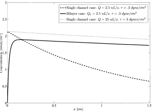
In Figure 2-2, model results for oxygen concentration at the cell surface for the bilayer and single channel case are shown. Using parameters for Case 2 and for flow rates

Q,

layer) with Qii = 25 nL/s in the upper channel, the oxygen concentration profile is nearly invariant along the length of the cell compartment except for a small zone of depletion in the initial region, due to the assumption of zero concentration in the inlet. If, instead of using a bilayer membrane device, cells were cultured in a single channel configuration with the maximum allowable flow rate, given

by

Q

of the channel. If we were to increase the flow rate in the single channel to a rate equal to that in the flow chamber of the bilayer (Q = 25 nL/s), we see a comparable concentration profile, though at the cost of greater shear (an increase from T = .3 dyne/cm2 to T= 3 dynes/cm2).

The concentration profiles in the channels themselves can be visualized using colormaps over the domain of interest. We see in Figure 2-3 that, with

Qj

2.5 nL/s and

Qjr

2, the concentration field in the cell compartment for the bilayer case is nearly uniform. For the single channel configuration operating again at a flow rate of

Q

along the length of the channel.

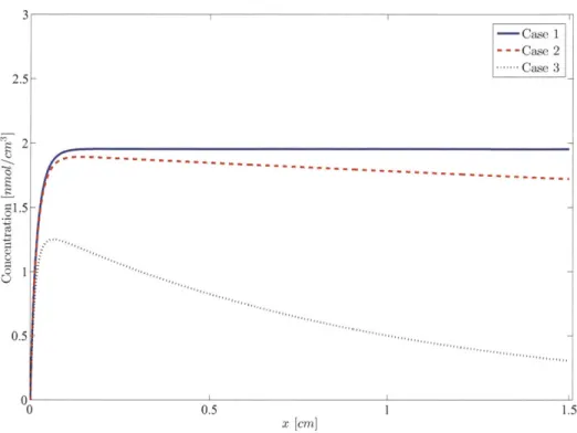
In Figures 2-4 and 2-5, we see the effect of changing the flow chamber flow rate

Qr

along the length of the channel. This is especially clear for Case 3, in which cells are both confluent and uptaking oxygen at a high rate: by increasing the flow rate in the upper chamber, the end-channel concentration for Case 3 is increased by a factor of about 3, so that, instead of a nearly 75% decrease in concentration along the 1.5 cm device length, we have only about a 29% decrease.

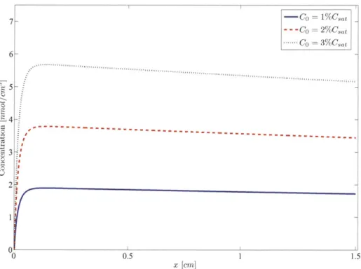
In Figure 2-6, we consider the effect of increasing the inlet concentration. As expected, as the inlet concentration is increased, the overall concentration profile increases.

Average Outlet Concentrations

In Figures 2-7, 2-8, 2-9, and 2-10, we show the effect of increasing the flow rate in the upper chamber (equivalent to modulating F) on the average outlet concen-trations for the single channel case and monoculture bilayer Cases 1, 2, and 3, respectively. For the single channel case, we see again the necessity of increasing shear in order to increase the outlet concentration. The same is not true for the single culture bilayer, in which the outlet concentrations are independent of the shear imparted on the cell layer.

2.6.2

Coculture Bilayer

We now consider the concentration profiles for the coculture bilayer configuration. In Figures 2-11, 2-12, and 2-13, we show the results of the model for cases in which the lower channel is cultured as in Cases 1, 2, and 3, respectively, with varying culture parameters in the upper channel. We see the considerable dependence of the lower channel's concentration profile on that of the upper channel.

Average Outlet Concentrations in the Coculture Bilayer Case

Finally, we present some of the results of the average outlet concentrations for the coculture bilayer case (Figures 2-14 and 2-15).

2.7

Discussion

The results presented in the previous section describe the range of operating pa-rameters that enable a bilayer microfluidic device to provide uniform, tailored levels of oxygen to various densities of cultured MSCs, while shielding cells from shear stresses induced by the flow rates that are necessary to transport solute along the device length. We have shown that, in the bilayer case, it is possible to achieve nearly uniform solute delivery without an increase in the shear stress to which the cells are exposed. Significantly, we have shown that the concentrations and hence, delivery profiles, are, except for a small entry zone, nearly uniform.

Of course, the extent of this entry zone can, in practice, be modified, too, by

varying the flow characteristics in both the cell compartment and the flow chan-nel. For example, we may consider a baseline case in which Q, = 10.0 nL/s and

Qr

Q[

Q",

a factor of about 4. Nevertheless, the above analysis, derived from simple first principles considerations, demonstrates the potential for the bilayer construct to deliver uniform profiles of solute to a culture of cells independently of the shear stresses that are exerted on the culture.

--- Single channel case: Q = 2.5 nL/s T = .3 dyne/cm2 -Bilayer case: Qj = 2.5 nL/s. r = .3 dyne/cm2

2.5- - Single channel case: Q = 25 nL/s r = 3 dynes/cm2

51.5

0.5

0

0 0.5 1 1.5

x [cm]

Figure 2-2: Concentration at the cell surface as a function of x, in units of nanomole per cm3_{: single channel (dotted and dashed lines) versus bilayer (solid black line). For the}

bilayer, the cell compartment flow rate is given by

Qj

while the flow channel flow rate is Qii = 25 nL/s. For the single channel, we have flow rates given by

Q

Q

profile, while the bilayer consumption profile is, except for a small depletion zone at the beginning of the channel, nearly uniform. Other parameters are those for Case 2.

C [nmol/cm:3 1 12 0 :0 0 0.5 1 1.5 x [cm]

(a) Single channel concentration field.

C1 [nnol/cm3]

,5x 103

0 0.5 1 1.5

x [cm]

(b) Bilayer concentration field.

Figure 2-3: Concentration fields for (a) single channel and (b) bilayer, in units of nanomole per cm3. In (a), we have the concentration field for the single channel

construct with

Q

compartment of the bilayer construct with

Q,

Q"1

The bilayer case demonstrates a far more uniform profile for a given flow rate and shear, while for the single channel configuration, the concentration of solute is depleted for much of the length of the channel. Other parameters are those for Case 2.

3 -- Case 1 - -- Case 2 Case 3 2.5-x [cm]

Figure 2-4: Concentration at cell surface as a function of x for cases 1, 2, and 3, in units of nanomole per cm 3 with

Qr

X [CM]

Figure 2-5: Concentration at cell surface as a function of x for Cases 1, 2, and

3, in units of nanomole per cm3 with

Q,

increasing the flow rate in the upper chamber by a factor of 5, the consumption profile becomes more uniform. In particular, for the high uptake rate and confluent seeding case (Case 3), increasing the flow rate in the upper chamber prevents depletion along the length of channel caused by high uptake of oxygen. The shear imparted on the cell culture is T = .3

dyne/cm

.

U0 0.5 1 1.5

x [cm]

Figure 2-6: Concentration at cell surface as a function of x in units of nanomole per cm3: Co varied as 1%Csat (solid blue line), 2%Cat (dashed red line), and 3%Cat (dotted black line).

Q,

Q"