HAL Id: hal-01298326
https://hal.archives-ouvertes.fr/hal-01298326
Submitted on 7 Apr 2016
HAL is a multi-disciplinary open access archive for the deposit and dissemination of sci-entific research documents, whether they are pub-lished or not. The documents may come from teaching and research institutions in France or abroad, or from public or private research centers.
L’archive ouverte pluridisciplinaire HAL, est destinée au dépôt et à la diffusion de documents scientifiques de niveau recherche, publiés ou non, émanant des établissements d’enseignement et de recherche français ou étrangers, des laboratoires publics ou privés.
stratified homogeneous turbulence
Alan Burlot, Benoît-Joseph Gréa, Fabien S. Godeferd, Claude Cambon,
Olivier Soulard
To cite this version:
Alan Burlot, Benoît-Joseph Gréa, Fabien S. Godeferd, Claude Cambon, Olivier Soulard. Large Reynolds number self-similar states of unstably stratified homogeneous turbulence. Physics of Fluids, American Institute of Physics, 2015, 27, pp.065114. �10.1063/1.4922817�. �hal-01298326�
Large Reynolds number self-similar states of unstably
stratified homogeneous turbulence
A. Burlot,1,2,a)B.-J. Gréa,1,b)F. S. Godeferd,2C. Cambon,2and O. Soulard1
1CEA, DAM, DIF, F-91297 Arpajon, France
2LMFA, Université de Lyon, École centrale de Lyon, CNRS, INSA, UCBL,
F-69134 Écully, France
(Received 23 April 2015; accepted 11 June 2015; published online 24 June 2015)
We study the influence of the large scale energy distribution on the long term dynamics of unstably stratified homogeneous turbulence at high Reynolds number Re = 106, using a statistical two-point spectral model based on the eddy-damped
quasi-normal closure. We consider several initial spectral scalings ksin the infrared
range with s ∈ [1; 5] and we establish that the resulting kinetic energy growth rates are controlled by s, with the appearance of backscatter effects for s ! 3.5. We then assess that only for s ≤ 4 do we observe self-similarity in the infrared and in the inertial ranges, but not in the dissipative range. Compensated energy and buoyancy spectra exhibit the expected Kolmogorov-Obukhov k−5/3scaling at long
time, and a trend to the theoretically predicted k−7/3scaling for velocity-buoyancy
cross-correlation spectrum thanks to the very large Reynolds number. We also show a direct link between the late-time anisotropy of the flows and the infrared spectrum, thus demonstrating long-lasting effect of initial conditions on unstably stratified turbulence. We show that, in addition to the Kolmogorov k−5/3scaling, the kinetic
energy spectrum inertial range includes a k−3 zone due to polarization anisotropy,
and we confirm the clear sin2θdependence of the velocity-buoyancy spectrum in the
inertial range, where θ is the orientation of the wave vector to the axis of gravity. However, an unexpected quick return to isotropy of the scalar spectra has been iden-tified, which cannot be explained by a standard dimensional analysis. C 2015 AIP Publishing LLC. [http://dx.doi.org/10.1063/1.4922817]
I. INTRODUCTION
In variable-density flows submitted to gravity, configurations in which an unstable density stratification induces turbulent mixing are encountered in several occurrences of industrial, geophys-ical, or astrophysical flows. Energy production by inertial confinement fusion also enters this flow category.1 Modelling the complete evolution of the time-dependent inhomogeneous buoyancy-induced mixing from the onset of the relevant instabilities (e.g., the Rayleigh-Taylor (RT) insta-bility) is rather complex as expressed by the variability of the mixing zone growth rates.2In order to shed light on the different mechanisms at work in the flow, one may simplify the problem by consid-ering unstably stratified homogeneous turbulence (USHT), wherein a continuous uniform density gradient feeds the flow dynamics.3–6This idealized framework was previously studied experimen-tally by Thoroddsen et al.7by means of a heated grid. The inquiry of mixing by buoyancy-driven turbulence was first introduced by Batchelor (1992)8and, since then, several models where estab-lished.9,10Considering the time evolution of flows from given initial conditions, the specific dy-namics of USHT, with respect to other distorted turbulence dydy-namics—e.g., homogeneous isotropic turbulence (HIT), stably stratified turbulence (SST), and rotating turbulence (ΩT)—resides in the
a)Electronic mail:alan.burlot@cea.fr b)Electronic mail:benoit-joseph.grea@cea.fr
growth of turbulent quantities due to the forcing of the mean density stratification. In the absence of additional sources terms, HIT, SST, or ΩT dynamics implies only a decay of energy, due to the nonlinear turbulent cascade and the dissipation.
The long time evolution of turbulent quantities in unstably stratified homogeneous turbulence leads to a self-similar regime.3As in RT instability11,12and homogeneous isotropic turbulence,13this terminal regime allows to express the energy spectrum as E(k,t) = u2(t)ℓ(t)G(kℓ(t)) with u(t) a
char-acteristic velocity, ℓ(t) a charchar-acteristic length scale, and G a dimensionless function. Multiple analyses were performed especially on HIT in self- or non-self-similar regimes (see, e.g., Meldi and Sagaut14 for an exhaustive review). A major result in both HIT and USHT is the role of large scale structures on the decay or growth of energy, and more specifically of large-scale dependence of two-point statistics, be it the velocity-correlation function f (r → ∞) or the low-wavenumber scaling of energy spectrum E(k → 0). For instance, one can assume the power law dependence lim
k→0E(k) → k
sto leading order;
in that case, the energy decay rate in HIT or growth rate in USHT can be estimated depending on s, which is commonly taken between 1 and 4. Classical cases investigated are Batchelor turbulence with s = 415and Saffman turbulence with s = 2.16,17Both cases were also studied in turbulence submitted to rotation,18stable stratification, or an externally applied magnetic field.19
In their recent analysis of freely decaying HIT experiments and modelling, Meldi and Sagaut14,20 discussed the availability of a long-time universal self-similar decay of energy with different scal-ings of the infrared (IR) spectral range—the energy spectrum range for wavenumbers k from 0 up to the spectral peak (which is located approximately at the inverse of the integral length scale). Only the value s = 1 seems to permit self-similar decay within all spectral ranges, and a second pivotal value s = 3.45 appears, as in the work by Lesieur and Ossia,13above which backscatter effects—a partial transfer of energy from inertial to large scales—do not allow the permanence of big eddies distribution.
In USHT, of course, no such decay is observed, and it is rather the growth rate which has to be investigated. From previous studies, it seems that it may depend on the initial distribution of large scales, but this was mainly assessed through the prism of amplified perturbations in a Rayleigh-Taylor mixing layer. As regards USHT with forced gravity and density gradient, recent studies4–6conclude to an exponential self-similar growth of turbulent kinetic energy as ∼ eβ N t; with
t the time, N the buoyancy frequency characterizing the constant acceleration and mean stratifica-tion, and β corresponding to the energy growth rate. Based on the arguments of Ref.3, an explicit relation between β and the IR power law s was also proposed in Ref.6when s ≤ 4 (or after a short transient when s > 4, since then the infrared spectral range adjusts rapidly to s = 4),
β = 4
s + 3. (1)
This permits to link the essential role of large scales with the dynamics of USHT. However, in addition to the IR scaling, it appears that large-scale anisotropy is also very important, in that it accumulates energy at wavenumbers orthogonal to the axis of gravity, a spectral domain where buoyancy forcing acts linearly on the initial large eddies when s < 4, but nonlinear interactions prevail when s = 4.3
Accordingly, high Reynolds number unstably stratified turbulence evolving self-similarly is required to study the influence of big eddies distribution on the statistics of the flow. Simulations for USHT have been recently proposed,5but there are limitations to the regimes direct numerical simulation (DNS) can reach. In USH or RT turbulence, not only the range of Reynolds numbers accessible with DNS is limited as in HIT, but also two other strong constraints apply: energy continuously grows due to the non zero vertical buoyancy flux, and a significant margin in the box size has to be preserved to accommodate the growth of the large scales, or, in other words, the infrared spectral range has to be wide enough. Altogether, the largest DNS realized to date (as, for instance, for RT21) reached a turbulent Reynolds number Re ≃ 5000, and were limited in time so that only a short similarity state period could eventually be accessed, and were obtained at a hefty computational price.
In HIT, significant computational power is required to reach turbulent regimes at relatively high Reynolds numbers. Statistical closures were successfully introduced in order to overcome this
limitation.22,23We, therefore, choose here also to tackle the problem at the level of the two-point statistics of turbulence, and hence use the eddy-damped quasi-normal Markovian (EDQNM) model for USH which has been developed and validated against DNS by Burlot et al.6Two-point statis-tical EDQNM modelling was already successfully used to represent homogeneous isotropic24and anisotropic turbulence in different contexts,25–27and was recently introduced for USH turbulence.6 It demonstrated its ability to reproduce properly DNS results in a range of parameters (Reynolds number, time span) accessible to the latter, and to provide adequate results at very large Reynolds number and asymptotically long times. The model permits to consider various parameters: initial spectral distributions, kinetic energy to buoyancy variance ratios, and Froude numbers. It gives ac-cess to the full scale-dependent anisotropic two-point statistics in the axisymmetric representation.
Our goal in the present study is to provide further insight about the influence of the initial large scale structures that force the evolution of USHT. In the EDQNM model, this consists in varying the power law ksof the infrared scale in the initial energy spectra. We propose to use our spectral
closure for USHT in order to explore large Reynolds number self-similar states and to explicitly investigate the link between the growth rate β and the slope s of the infrared spectra, extending3,5 to new parametric ranges. We pursue the analysis of self-similarity properties not only in the large scales but also in the inertial and the dissipative ranges to seek the existence of universal scaling laws. Therefore, the question raised is which scales of USH turbulence keep a memory of its gener-ating initial conditions. In parallel, the anisotropy of the turbulent structures will be scrutinized in order to measure the influence of the buoyancy force.
The paper is organized as follows. First, we present the unstably stratified homogeneous turbu-lence configuration in Sec. II along with its governing equations, the EDQNM closure, and the initial conditions and parameters. Then, numerical results are discussed in Sec.III: non-dimensional numbers in Sec.III A, one-point statistics in Sec.III B, the time evolution of spectra in Sec.III C, and finally anisotropic characterization of velocity and buoyancy distributions in Sec.III D. Final comments and conclusions are provided in Sec.IV.
II. UNSTABLY STRATIFIED HOMOGENEOUS TURBULENCE
We first present in this section the dynamical equations for USHT written in terms of buoyancy, then we provide a quick description of the spectral closure model which is used to compute the long time statistics of the flow in a high Reynolds number self-similar regime. The reader can refer to Burlot et al.6for a complete description.
A. Dynamical equations for unstably stratified homogeneous turbulence
We consider an incompressible flow in which turbulent quantities are assumed statistically homogeneous and axisymmetric about the vertical axis which bears gravity. The mean flow ⟨u⟩ is assumed to be zero, whereas the fluid density has a uniform linear mean gradient in the vertical direction, which is assumed to be unchanged by density fluctuations. In addition, the contrast of density is supposed small allowing the Boussinesq approximation. The resulting buoyancy force is destabilizing when gravity and density gradients are of opposite sign, producing the unstably strati-fied situation. The following Navier-Stokes-Boussinesq equations are written for the divergenceless fluctuating velocity fieldu and for ϑ, the fluctuating buoyancy rescaled as a velocity:
∂ui ∂xi =0, (2a) ∂ui ∂t +uj ∂ui ∂xj =−∂p ∂xi + ν ∂ 2u i ∂xj∂xj +Nϑδi3, (2b) ∂ϑ ∂t +uj ∂ϑ ∂xj =D ∂ 2ϑ ∂xj∂xj +Nu3, (2c)
where p is the pressure divided by a reference density, ν the kinematic viscosity, and D the molec-ular diffusivity. The intensity of stratification is set by the buoyancy frequency N by analogy with
the Brunt-Väisälä frequency in the stably stratified case. The stratification time scale associated with the linear buoyancy term in Eq. (2b) is therefore TN =1/N.
For a flow periodic in all three directions, Eqs. (2a)–(2c) can be solved using classical pseudo-spectral discretization techniques,28 but such direct numerical simulations are computationally demanding. Moreover, in DNSs of stratified homogeneous turbulence, the velocity and buoyancy fields are post-processed to provide, e.g., two-point statistics such as energy spectra. We propose to use instead a model that solves equations for the two-point statistics. The outline of the correspond-ing spectral closure is described hereafter.
B. Spectral closure
An overview of the closure is given in this section. For a complete description, the reader may refer to the lecture given by Orszag24for the isotropic case, to Cambon et al.,26Sagaut and Cambon29for the anisotropic axisymmetric configuration, and to Ref.6for the specific adaptation to unstably stratified homogeneous turbulence.
Instead of considering the velocity and buoyancy fields whose dynamics is ruled by Eqs. (2a)–(2c), one considers their two-point correlation functions, ⟨u(x)u(x + r)⟩ for velocity, ⟨ϑ(x)ϑ(x + r)⟩ for buoyancy, and ⟨u(x)ϑ(x + r)⟩ for their cross-correlation. They do not depend on the loca-tionx in homogeneous turbulence, but indeed depend on the orientation of the separation vector r in anisotropic flows. Dynamical equations for these two-point statistics can be obtained from Eqs. (2a)–(2c), but are unclosed since they involve two-point triple correlations, as widely known. This issue related to the hierarchy of statistical moments is solved in the present work by using the eddy-damped quasi-normal Markovian closure which permits to express triple correlations in terms of second-order ones. The model provides closed equations for spectra of the above-mentioned correlation functions, transforming the dependence on the separation vectorr in physical space into a dependence on the wave vectork in the Fourier representation. We shall use the following spectra arising from the two-point correlations statistics.
• The Reynolds stress tensor spectrum Ri j(k) such that Ri j(k)δ(k + k′) = ⟨ ˆui(k) ˆuj(k′)⟩ where ˆui
denotes the Fourier coefficient of velocity component uiand δ being the 3D Dirac function.
• From that the kinetic energy spectrum can be defined as E(k) = Rii(k)/2 assuming summation
over the repeated index i.
• The buoyancy spectrum B(k) with B(k)δ(k + k′) = ⟨ ˆϑ(k) ˆϑ(k′)⟩ with similarly ˆϑ the Fourier
coefficient of ϑ.
• The co-spectrum of vertical velocity-buoyancy two-point correlation, F (k), which is defined from F (k)δ(k + k′) = ⟨ ˆu3(k) ˆϑ(k′)⟩.
In order to obtain the EDQNM closed equations for Ri j, E, F , B, Eqs. (2a)–(2c) are Fourier
transformed. This helps to eliminate pressure by using incompressibility stated in Fourier space: k · ˆu = 0. The dynamical equations for the two-point spectra are obtained by multiplication by ˆu(k) and ˆϑ(k) and taking the ensemble average ⟨ ⟩. The classical turbulence problem of the hierarchy of dynamical equations occurs then, with second-order moments involving third-order moments. The core idea of the EDQNM closure is to assume that third-order moments are linearly relaxed by fourth-order cumulants, which are the departure of the fourth-order statistics from that of a Gaussian distribution. Formally, this provides an expression of the third-order moment involv-ing only products of second-order moments, and hence a set of closed dynamical equations for second-order statistics, namely, the desired spectra.
In USH turbulence, in addition to the quasi-normal assumption, one introduces a second hypothesis on the third-order moments whose dynamics is enriched by explicit buoyancy and stratification terms in the dynamical equations. These terms, which are ignored in Ref. 30, are explicitly accounted in Ref.31for the stable stratification case. Here, we use the simple assumption that nonlinear contributions of stratification-related terms in the dynamics of third-order moments can be replaced by an additional damping to nonlinear terms following the successful procedure described in Ref.6and supported by DNS results.
In the end, one obtains a set of coupled integro-differential equations whose discretization yields the evolution in time of the spectra for Nk discretized wavenumbers k in the range [km,kM],
and for Nθ polar orientations θ of the corresponding wave vector k about the axis of gravity.
For instance, θ = 0 corresponds to motion perpendicular to the axis of gravity (k being aligned with gravity, and from incompressibilityk · ˆu = 0). Axisymmetry permits to analytically integrate the spectra over the azimuthal angle. The output of EDQNM computations is therefore a set of Nk× Nθ discrete values of velocity, buoyancy, and flux spectra distributed in Fourier space with a
polar-spherical mesh.
All the following computations were done using Nk=128 discretized wavenumbers k between
km=10−2 and kM=104 and Nθ =21 polar angles. The logarithmic distribution of ks therefore
allows for ∼20 wavenumbers per decade, which is well above the already comfortable value of 10 wavenumbers per decade recommended for isotropic EDQNM resolution. We checked wavenumber convergence using 512 and 1024 points in order to evaluate if long range interactions could modify the solution, without observing any noticeable change. No further dependence is observed when varying the angular discretization.
It is convenient to work with spherically integrated spectra obtained by integration of k-or (k,θ)-dependent spectra Ri j(k, θ), E(k, θ), B(k, θ), and F (k, θ) over all orientations of k. In
doing so, one only retains a global effect of anisotropy at each scale corresponding to a given wavenumber k (again, the model is capable of full axisymmetric description). We shall denote Ri j(k), E(k), B(k), and F(k) the corresponding spherically integrated spectra (for instance E(k) =
2πk2!π
0 E(k,θ) sin θ dθ).
C. Varying the initial distribution of big eddies
As previously done in isotropic turbulence using the EDQNM closure,13 we investigate the evolution of USHT starting with different distributions of the big eddies, that is, we study the influence of the large scales spectral distribution on energy growth rate and flow anisotropy. With respect to isotropic turbulence, two additional parameters need to be introduced: the initial ratio of buoyancy variance to kinetic energy, as a trace of the way stratification is introduced in the flow (for instance, in heated grid turbulence the corresponding initial buoyancy variance is very small7); and the Froude number that quantifies the intensity of stratification with respect to inertial effects.
We tune these parameters using the analytical spectral distribution for kinetic energy32 E(k,t = 0) = As ! k kpeak "s exp ! "− s 2 ! k kpeak "2 # $, (3)
where k is the wavenumber, kpeakis the most energetic wavenumber, s is the slope of the infrared
spectra, and Assets the total initial kinetic energy K (t) =
!+∞
0 E(k,t) dk. Along with a choice of
kinematic viscosity ν = 5 × 10⁻⁴, the kinetic energy is used to compute the initial Reynolds number
as Re = K2/(εν), where kinetic energy dissipation is ε(t) = 2ν!+∞
0 k2E(k,t) dk. Spectra as in Eq. (3)
are used to initialize the buoyancy spectrum B(k,t = 0), and the initial flux is F(k,t = 0) = 0. The Froude number is then obtained as Fr = ε/(K N) where N is the buoyancy frequency. The larger Fr, the more important the intensity of stratification, and thus the buoyancy force. The third non-dimensional parameter is Λ = ⟨ϑϑ⟩ /K which we choose to be Λ = 1 at the beginning of all the simulations. Here, the buoyancy variance is related to its spectrum as ⟨ϑϑ⟩ (t) =!+∞
0 B(k,t) dk.
We have checked that the precise value of Λ has no influence on the asymptotic similarity state, only on the transient short-time growth. The initial parameters for the computations are as follows: the Reynolds number is Re = 833 and the Froude number is Fr = 1.2. The corresponding spectral peaks for each value of the infrared power law kswith s from 1 to 5 are detailed in Table I. The
corresponding initial spectra are shown as a subset of curves in Figs. 3(a)and 3(b). From these initial narrow-band spectra, turbulence develops an inertial range and a dissipative one, with or without adjustment of the infrared range energy distribution. As observed in Figure3, the infrared range spans almost four decades, so that the large scale cutoff has negligible effect, unlike what may be observed in DNS at long time, even at high resolution.
TABLE I. Peak wavenumbers for each power law s chosen in our nine simulations, and non dimensional final time N t, at which Re = 106.
s 1 1.5 2 2.5 3 3.5 4 4.5 5 kpeak 34.64 37.95 40 41.4 42.43 43.2 43.82 44.32 44.72
N t 9.4 10.4 11.9 13.1 14.5 16.2 16.9 17.4 17.6
Finally, the computations are carried out until Re = 106 for each case, corresponding to a
different final time Nt as shown in TableI.
III. NUMERICAL RESULTS
We analyse here the parametric influence of the IR power law s on the dynamics of USH turbu-lence, in particular on one-point statistics which are obtained by integrating the spectra over the complete spectral space. In Sec.III A, we first discuss the flow regime characterized by Reynolds and Froude numbers, and by the mixing parameter Λ, then the evolution of kinetic energy, buoy-ancy and vertical flux variances in Sec.III B. Second, we shall discuss in Sec.III Cthe observed similarity in the time-dependent spectra, and the evolution of inertial and infrared ranges.
A. Flow regime characterized by Re, Fr, and Λ
The time evolution of the three non-dimensional parameters characterizing the flow is shown in Figure1in terms of non-dimensional time t∗=Nt.
First, the transient phase is similar to the one described in Ref.6: at short time, the flow adjusts in the small scales and the Reynolds and Froude numbers decrease, as a result of the transfer of kinetic energy from large to small dissipative scales. The transient decrease stops after about 2 stratification periods, and a monotonic asymptotic behaviour is observed, starting at t∗≃ 5.
The Reynolds number (Figure1(a)) reaches a long-time exponential behaviour, evolving more rapidly for low values of s than for larger ones. All runs start from Re = 833 to finally reach Re ≃ 106. (Note that due to the exponential growth, computational time becomes long due to the
extremely low time step δt∗∼ 10−7.) The Reynolds number growth depends on the initial
condi-tions: the shallower the spectrum, the sooner the self-similar state is reached. Self-similarity starts uniformly around Re = 2 × 10³but occurs from t∗≃ 3 for s = 1 to t∗≃ 6 for s = 5. We notice the
same exponential growth for s ≥ 4. This is correlated to the evolution of kinetic energy whose growth rate is bounded by the infrared slope s = 4 due to backscatter effects (see below).
In all cases, the Froude number (Figure1(b)) which starts above unity (Fr = 1.2 for all runs), corresponding to weakly stratified flow, eventually reaches an asymptotic value lower than unity, showing that the flow dynamics is therefore significantly altered by stratification. This attests of the equilibrium between buoyant and inertial forces. Final values are spread between Fr = 0.3 for s = 1 and Fr = 0.48 for s ≥ 4. This asymptote of Froude number indicates the grip of stratification effects
FIG. 1. Non-dimensional parameters evolution: (a) Reynolds number Re = K2/(νε); (b) Froude number Fr = ε/(N K );
on the flow which is stronger when the infrared slope is lower. It is explained by the energy of large scales structures which is more important for s = 1 than s = 4, is less submitted to non-linear transfer than linear buoyancy force. Furthermore, we observe that the maximum asymptotic Froude number is reached for s = 4 where Fr = 0.48. Increasing s further does not seem to produce a decrease of the asymptotic Froude number.
Finally, the time evolution of the mixing parameter Λ is presented in Figure1(c). All runs start with Λ = 1, meaning there is exact equipartition between buoyancy variance and kinetic energy. The short-time depletion of Λ is expected as in stably stratified turbulence, because the cascade of scalar is more efficient than the turbulent energy cascade. Later, one expects a self-similar mixing regime characterized by a plateau of Λ. However, Figure1(c)shows that after reaching a peak value, at long time Λ evolves slowly, but nonetheless decays. The asymptotic value is rather concentrated, between Λ = 1.6 for s = 1 and Λ = 1.3 for s = 5. This means that the flow contains 30%–60% more buoyancy variance than kinetic energy in its asymptotic regime. Here again, the large-scale distribution with a slope s = 4 seems to mark a limit of mixing efficiency in USH turbulence.
B. Energy and flux self-similar growth
Figure2shows the time evolution of kinetic energy K , buoyancy variance, and vertical buoy-ancy flux ⟨u3ϑ⟩ =!0+∞F(k)dk. The exponential growth eβ N t, with β defined by Eq. (1), expected
in the self-similar regime, is plotted for each case with dashed lines. Clearly, all our simulations exhibit the self-similar regime for kinetic energy and buoyancy variance evolution, and for the flux. For these three quantities, the asymptotic growth is fastest for the lowest infrared slope s = 1, and decreases with increasing s. A saturation of this increase is observed at large s above s ≃ 4, say, which is explained by backscatter effects observed in the energy and transfer spectra in Figures3(a)
and4, discussed in Sec.III C.
We compare in TableIIthe theoretically predicted asymptotic growth with the measured one from the time evolution of kinetic energy K (t), buoyancy variance ⟨ϑϑ⟩(t), and vertical buoyancy flux ⟨u3ϑ⟩(t). For all three quantities, the growth rate is in very good agreement with the theoretical
value for all cases of s ∈ [1; 4]. This also demonstrates that sufficiently long computations are needed to recover the right exponent, which should not be measured earlier than Nt ≃ 6.
C. Detailed spectral adjustments
Our aim in this section is to discuss the turbulent dynamics from the point of view of the large scales—the infrared range—on the one hand, and of the inertial range, on the other. These are discussed in the respective Secs.III C 1andIII C 2, where similarity formulas are applied to expose each range.
The spherically integrated spectra E(k), B(k), and F(k) are plotted in Figures3(a),3(b), and
3(c), respectively. It shows the initial time distribution of kinetic energy and buoyancy (initial flux is zero), as well as their state when the flow reaches a very high Reynolds number Re = 106. It can be
seen at first sight that the energy and the buoyancy spectra evolve to a similar Kolmogorov-Obukhov
FIG. 2. (a) Kinetic energy, (b) buoyancy variance, and (c) vertical buoyancy flux evolution with slope of self-similar regime. Dashed lines represent the theoretical self-similar dynamics based on the formula K (t) ∼ exp(βN t) with β given by Eq. (1).
TABLE II. Values of β at the end of each computation for the kinetic energy, the buoyancy variance, and the scalar flux compared to the theoretically predicted one from Eq. (1), βt h, which is identical for the three quantities. The different
instantaneous growth rates are obtained in the simulations from βX= 1 X
dX dN t.
s βth βsimK βKsim/βth(%) βsim⟨ϑϑ⟩ β⟨ϑϑ⟩sim /βth(%) β⟨usim3ϑ⟩ β⟨usim3ϑ⟩/βth(%)
1 4/(1+3) 0.993 99.3 0.989 98.9 0.994 99.4 1.5 4/(1.5+3) 0.885 99.5 0.881 99.2 0.886 99.7 2 4/(2+3) 0.797 99.6 0.794 99.3 0.798 99.7 2.5 4/(2.5+3) 0.724 99.6 0.722 99.3 0.725 99.7 3 4/(3+3) 0.663 99.5 0.661 99.2 0.664 99.6 3.5 4/(3.5+3) 0.610 99.1 0.609 98.9 0.610 99.2 4 4/(4+3) 0.572 100.2 0.571 99.9 0.572 100.1 4.5 4/(4+3) 0.570 99.7 0.568 99.4 0.570 99.7 5 4/(4+3) 0.573 100.3 0.571 100.0 0.573 100.2
k−5/3 scaling, while the buoyancy flux follows roughly a k−7/3 scaling law in the inertial range.
The dissipative ranges are also very similar, but by contrast the infrared range that feeds the energy cascade is much different. Indeed, among the initial 9 different values chosen for s, the infrared distributions of spectra at s = 4, 4.5, and 5 rejoin to a single k4 distribution in the large scales.
The infrared zones of the spectra at s = 4.5 and 5 have therefore evolved to Batchelor-type infrared spectra with s = 4. The well-known backscatter effects rearrange in a few eddy turnover times the energy distribution at large scale.33 This effect can be more visible on large-scale compensated spectra in Sec. III C 1, but can also be demonstrated by examining the kinetic energy transfer spectra of Figure4, that is, the transfer spectra T(k) for the spherically integrated spectrum E(k) (whose dynamics would follow a Lin type equation).34The figure shows that, even in this highly anisotropic flow, energy transfer in USH turbulence consists of a strong downscale transfer with negative transfer in the large scales and positive transfer in the small ones. Both regions are sepa-rated by a well-defined inertial range in which the energy flux is constant, due to the very high Reynolds number regime. However, when closing up on the very large scale region, at smaller wavenumbers, the inset in Figure4shows the existence of backscatter of energy in the large scales for s > 2, although of small amplitude compared with the forward cascade. The observed threshold s = 2 corresponding to the dominance of backscatter term in the transfer is coherent with distant interaction expansion of the EDQNM closure shown by Ref.33. The backscatter is largest for s ≥ 4 and explains the rapid recovery of Batchelor scaling k4if the turbulent infrared range initially scales
as ks with s > 4. In addition, the importance of distant interaction between modes for backscatter
dominated transfers can be verified by T(k) ∼ k4 for k → 0 in Figure4as already mentioned in
Lesieur33and Soulard et al.3
FIG. 3. Initial spectra (bottom set of curves in each panel, divided by 10) and spectra (top set) at Re = 106of: (a) kinetic
energy E(k); (b) buoyancy variance B(k); and (c) buoyancy–velocity cross-correlation F(k). Each set of curves represents simulations with s from 1 to 5. The straight lines indicate the inertial range scaling k−5/3for E(k) and B(k) and k−7/3for
FIG. 4. Left: k-weighted kinetic energy transfer spectrum normalized by its maximum value kT (k)/max(|kT (k)|) for the different cases at s = 1 to 5 and Re = 106. (The area beneath the curves is proportional to the transfer in this lin-log
representation.) Right : A close-up of the rectangle shown with dashed lines in the small k region. Inset: Log-Log representation of renormalized transfers T (k)/T (km) showing typical k4scaling for s > 2 due to backscatter effects.
1. Large scale adjustment in the infrared spectral range
Figures5and6, respectively, show the large-scale compensated spectra for the kinetic energy E(k) on the one hand, and for the buoyancy variance B(k) and the vertical buoyancy flux F(k) on the other. The rescaling formula is
X∗ infrared(k,t) = X(kX(k,t) m,t) × ! k km "−s , (4)
where X is replaced by E, B, and F successively, and km is the smallest wavenumber of the
simulation. Equation (4) is an adaptation of the classical formula used in isotropic turbulence.13,35 By applying rescaling (4), one compensates the growth of energy or flux (the division by X(km,t))
and transforms to a plateau the infrared range assumed to scale as ksat each time. Departure from
horizontal means a departure of the infrared spectral range from its initial distribution.
For ease of presentation, kinetic energy spectra in Figure5are plotted only for runs using s = 1, 2, 3, 3.5, 4, and 5, in semi-log scale.
FIG. 5. Large-scale spectrum of kinetic energy E(k) compensated using Eq. (4) at integer intermediate times from t∗=0 to
the last time given in TableI. Increasing times as indicated by the arrows. The last computed spectrum is indicated by symbols (red color online) and corresponds to different times given hereafter for the different cases: (a) s = 1 (last time t∗=9.4); (b)
s =2 (t∗=11.9); (c) s = 3 (t∗=14.5); (d) s = 3.5 (t∗=16.2); (e) s = 4 (t∗=16.9); and (f) s = 5 (t∗=17.6). (Note that in panel (f), the initial spectrum at t∗=0 is initially k5and compensated by ∼ k−4, so that it gets out of the figure, but quickly
FIG. 6. Large-scale spectrum of buoyancy variance B(k) compensated using Eq. (4) at the same times t∗as in Figure5,
for: (a) s = 1; (b) s = 3; (c) s = 5. And the compensated spectrum F(k) of velocity-buoyancy correlation for: (d) s = 1; (e) s =3; (f) s = 5. (Note that, as in Figure5(f), for panel (c) the initial curve for B(k) gets out of the plot for the same reason; moreover, the initial fluxes at t∗=0 in panels (d)–(f) are initially zero.)
In Figures5(a)and5(b), for s = 1 and 2, the compensated kinetic energy spectrum exhibits a plateau in the first two decades of k at all times, so that the infrared energy scaling does not change at all. For s = 3 in Figure5(c), one observes that the infrared slope begins to depart slightly from the initial k3dependence, and for s = 3.5 in Figure5(d), it is clear that the similarity of large scales
is not valid anymore since s increases towards 4, unlike cases s = 4 (Batchelor turbulence) and 5 in Figures5(e)and5(f), where the infrared slope decreases slightly. Finally, for s = 5, we observe a quick reshape of the spectra in the region connecting infrared and inertial ranges—the observed bump near k ∼ 50 in the early times in Figure5(f)—such that the spectrum eventually recovers an almost identical evolution as for the case s = 4 due to backscatter. In a study of isotropic turbulence using the EDQNM model, Lesieur and Ossia find a limit s = 3.45 above which backscatter appears and the infrared scaling evolves in time.13This is consistent with what we observe here in USH turbulence.
The same comments apply for the evolution of the buoyancy variance spectrum B(k) and the vertical buoyancy flux F(k), plotted, respectively, in Figures6(a)-6(c) and 6(d)-6(f) only for cases s = 1, 3, and 5 for the sake of brevity. This denotes that the dynamics of kinetic energy and buoyancy variance are closely intertwined.
To summarize, the EDQNM simulations allow to assess the importance of backscatter in the growth of turbulent quantities of USHT. The predictions established by Eq. (1) assume negligible backscatter effects and accordingly are valid for s ≤ 4. However, backscatter still has an influence around s = 3.5 by slowly modifying the similar distribution of energy at large scales although dominated by buoyancy production. Observe that the predictions given by Eq. (1) in Table II
slightly overestimate the growth rates particularly around s = 3.5. This tendency can be interpreted as evidence of backscatter influence.
2. Inertial range scaling
We focus here on the inertial range in the spectra, by renormalizing them as for classical Kolmogorov–Obukhov turbulence, using the kinetic energy dissipation ε(t) and buoyancy dissipa-tion εB(t),
E∗
inertial(k,t) = E(k,t) × ε(t)−2/3k5/3, (5a)
B∗ inertial(k,t) = B(k,t) × εB(t)−1ε(t)1/3k5/3, (5b) F∗ inertial(k,t) = F(k,t)N−1 % CKε(t)1/3+COεB(t)ε(t)−2/3 &−1k7/3, (5c)
FIG. 7. Inertial range compensated spectra from Eq. (5a) for kinetic energy E(k): (a) s = 1; (b) s = 2; (c) s = 3; (d) s = 3.5; (e) s = 4; and (f) s = 5. Times are as in Figure5, and the latest spectrum is denoted with symbols (red color online). (Note that the initial narrow-banded spectra get out of the plots but are indicated for better appreciation of the time evolution.) Vertical lines locate the wavenumbers kℓ, kO, and kηcorresponding, respectively, to the integral length scale, to the Ozmidov scale
and to the Kolmogorov scale for this last spectrum.
with the classical inertial power law −5/3 for the kinetic energy spectrum E(k) and for the buoyancy spectrum B(k) as suggested by dimensional analysis.36,37We also choose −7/3 for the buoyancy-velocity co-spectrum F(k), following experimental measurements in grid turbulence38and theoretical predictions of Ref.39. The dependence on dissipation in Eq. (5c) is obtained by assuming equilibrium between non linear terms and production in the equation for the vertical buoyancy flux spectrum as in Ref.40. Here, CK and COcorrespond, respectively, to the Kolmogorov and Obukhov constants.
Figure7shows these compensated spectra for E(k), and Figure8for B(k) and F(k). Figures 7(a)-7(f)show that the rescaled kinetic energy spectrum E∗
inertial(k) evolves similarly
for all infrared power laws s. On these plots, the rescaled initial spectra (curves that do not fit
FIG. 8. Inertial range compensated spectra from Eqs. (5b) and (5c) for the buoyancy variance spectrum B(k): (a) s = 1; (b) s = 3; (c) s = 5. Same for the co-spectrum of buoyancy-velocity F(k): (d) s = 1; (e) s = 3; (f) s = 5. Times as in Figure5, and the latest spectra are denoted with a heavy line and symbols. As in Figure7, integral-, Ozmidov-, and Kolmogorov-length-scale-related wavenumbers kℓ, kO, and kηare indicated for the last spectra.
within the chosen vertical range) are largely above the later time spectra, since dissipation is not fully built at the earliest times of computation. After a short transient during which the similarity shape evolves, the rescaled spectra develop three characteristic features. First, the inertial range zone corresponds to a plateau at intermediate wavenumbers, at a value slightly above the commonly admitted value CK ≃ 1.4 for the Kolmogorov constant. This is consistent with isotropic EDQNM
choosing a0=0.36 in the eddy damping term.41Second, the spectral region close to the integral
scale wavenumber (kℓ∼ 1) exhibits a rather narrow peak different from the classical compensated
spectrum in HIT. Indeed, as predicted for RT turbulence by Soulard,42a modification of the spectra near the integral scale at k ∼ 1 is expected to scale as k−3in the inertial range zone delimited by
the integral scale and the Ozmidov scale (with the corresponding Ozmidov wavenumber classically defined as kO=N3/2/ε1/2). Note that strong differences between RT and USH turbulence prevail
at large scales due to inhomogeneous specificities of RT. However, for smaller scales of the inertial range, it seems reasonable to seek same scaling laws between RT and USHT. Third, the observed bump at the upper end of the inertial region is the classically observed bottleneck in turbulence, from the depletion of non-linearity when reaching the dissipative range.
Rescaled buoyancy spectra, shown in Figures8(a)-8(c) only for s = 1, 3, 5, evolve towards a self-similar shape, as for the rescaled kinetic energy spectra: the inertial k−5/3 scaling appears
through a plateau at the Obukhov constant CO≃ 0.7.43This value is consistent with the analysis of
isotropic EDQNM for passive scalar with a single eddy damping term proposed by Ref.44. The plateau lies between the peak observed at the wavenumber kℓ∼ 1 defined by the integral length
scale, and the accumulation bottleneck between the end of the inertial subrange and the dissipative one. In B∗
inertial(k), the latter bump is much more pronounced than in Einertial∗ (k) in Figures7(a)–7(f).
This is also observed in passive scalar spectra in grid turbulence experiments.45 Finally, Figures8(d)-8(f)show the velocity-buoyancy co-spectrum F∗
inertialfor the same s = 1, 3,
5. We observe a rapid drop in time of this rescaled flux from the initial conditions, before it settles to its self-similar shape. As for kinetic energy and buoyancy spectra, the inertial range is flanked by the peak at integral scale and the bottleneck. The inertial range seems to follow more loosely the k−7/3
anticipated scaling, since, unlike E∗
inertialand Binertial∗ , the convergence towards k−7/3is much slower,
in terms of Reynolds number. (Lower Reynolds number runs, not presented here, also present this feature.) This may explain as well the difference of plateau level compared to Ref.40which is based on low Reynolds number Rayleigh-Taylor simulations. Moreover, the velocity-buoyancy flux is a cross-correlation statistics whose convergence is indeed expected to be slower than that of autocor-relation spectra. Finally, buoyancy acts at all ranges, and may disrupt the expected flux equilibrium in the inertial range. We recall that the energy cascade in this range is submitted to both the linear buoyancy force, and to the nonlinear triadic transfer.
D. Anisotropy variation with s
As mentioned, the dynamics of USH turbulence is strongly linked to the flow anisotropy which is produced by plumes from the effect of the buoyancy force. Hence, vertical kinetic energy is larger along the direction of gravity, along which the flow structures are elongated. Not only is the velocity field anisotropic, but also the density field, so that the description of their anisotropic structure requires specific quantities. We start in Sec.III D 1by characterizing the anisotropy of the Reynolds stress tensor ⟨uiuj⟩ by computing its deviatoric part bi j=⟨uiuj⟩/⟨uiui⟩ − δi j/3, δi j being the
Kro-necker tensor components. This provides a simple global view of the flow anisotropy at large scales. Then, we propose in Sec. III D 2 a refined description that permits a scale-by-scale evaluation of anisotropy, both for velocity and density fields, especially in the infrared subrange of interest.
1. Anisotropy in the self-similar regime
The first characterization of kinematic anisotropy is done with the anisotropy in the Reynolds stress components through its deviatoric tensorb. From axisymmetry (b11=b22) and
incompress-ibility (bii=0), only one component ofb is required; we choose to compute b33=⟨u3u3⟩ / ⟨uiui⟩−
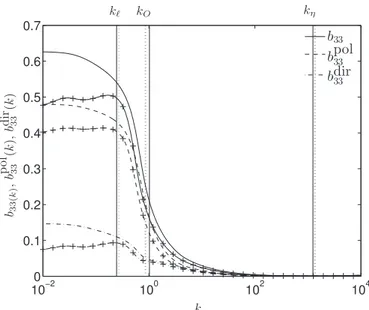
FIG. 9. One-point statistics of anisotropy: (a) vertical component of the Reynolds stress tensor anisotropy b33for the different
infrared range power laws ks, with s from 1 to 5; (b) comparison for cases at s = 2 and 4 (indicated by +) between b 33and
its polarization and directivity components bpol33 and bdir 33.
developing in the flow. Its evolution in time is shown in Figure9(a)for the different s cases. The figure shows that, starting from b33=0 for isotropic turbulence, b33grows rapidly and settles at an
asymptotic value that depends on the infrared power law s: between 0.42 for s = 1 and 0.32 for s = 5. The different levels of anisotropy in the self-similar regimes at different s clearly show the dependence of the late-time structure of USH dynamics on initial conditions in the large scales. In mixing zones generated by the Rayleigh-Taylor instability, different levels of anisotropy as a func-tion of the growth rate in the self-similar regime have been observed, see Gréa.46This is consistent with what we show here, that it is possible to reach a range of final regimes by modifying the initial energy distribution at large scale.
As recalled in Sagaut and Cambon,29the Reynolds stress tensor can be decomposed as ⟨u
iuj⟩ =
⟨uiuj⟩iso+⟨uiuj⟩pol+⟨uiuj⟩dir with ⟨uiuj⟩iso the isotropic contribution over which the two
aniso-tropic contributions are superimposed: ⟨uiuj⟩polthe polarization part and ⟨uiuj⟩dirthe directionality
part. Accordingly, b33can be split in two components as well: b33=bpol33 +bdir33 (logically biso33 =0
from the definition of ⟨uiuj⟩iso). This decomposition permits to identify two sources of anisotropy
coming from the structuring of the flow. First, the directionality contents testify of the accumulation of kinetic energy for wave vectors in the axial (i.e., along the axis of gravity) or the perpen-dicular direction. Second, the polarization part assesses the kind of structures that are produced once directional anisotropy has set in. For instance, an axisymmetric flow may contain mostly sheet-like (as in stably stratified turbulence31), jet-like structures (as in conducting fluid turbulence in a permanent background magnetic field27), or vortex-like ones (as in rotating turbulence26). In the USH case, the large directional anisotropy observed in Figure9(b) attests a two-dimensional tendency. It can be shown that a purely two-dimensional flow settles an upper limit to the directional anisotropy at bdir
33=1/6. Furthermore, one also needs to examine the polarization in order to fully
qualify the flow structure: it contains three components when bpol33 =0, but corresponds to an exactly two-dimensional two-component flow (vortex like) if bpol33 =−1/3. Values in between attest of pref-erential trends. On the contrary for RT or USH flows, the strong polarization anisotropy (bpol33 =1/3) (see Figure9) points out more precisely the dominance of vertical jet-like structures.
One expects that the polarization part represents 80% of the total velocity anisotropy in USH turbulence as from RT47 or previous USHT5 simulations. We confirm this with the plot of b
33
compared to bpol33 and bdir
33 in Figure9(b)for the cases s = 2 (Saffman turbulence) and 4 (Batchelor
turbulence). The asymptotic ratio bpol33/b33indeed reaches 80% in both, even though b33does not
asymptote exactly to the same value. This is observed in all the cases we computed independent of the large scales distribution. Figure9(b)therefore shows that directional anisotropy is moderate compared to polarization anisotropy, but the value ∼0.3–0.4 reached by their sum indicates an overall strongly anisotropic flow with preferential motion along the axis of gravity. We characterize further this anisotropy by examining its scale distribution in Sec.III D 2.
FIG. 10. Scale-by-scale deviatoric part b33(k) of the Reynolds stress tensor component R33=⟨ ˆu3ˆu3⟩ and its polarization and
directional contents bpol33(k) and bdir33(k) as a function of wavenumber k, for USH turbulence at s = 2 and 4 (indicated by +)
for the same value of the Reynolds number Re = 106. The vertical lines indicate wavenumbers corresponding to the integral,
Ozmidov, and Kolmogorov length scales kℓ, kO, kη, respectively (dashes for the case at s = 4).
2. Scale-by-scale anisotropy characterization
We first investigate the anisotropy of b33 scale-by-scale, by computing its value at each
wavenumber k, and its polarization and directional contents. These are shown in Figure10for s = 2 and 4. The figure first shows that maximal anisotropy b33(k) ≃ 0.5–0.6 is reached in the large scales.
It starts decreasing abruptly for wavenumbers larger than that corresponding to the integral length scale k < kℓ—i.e., for structures smaller than the large energy-containing eddies—down to zero at
the end of the inertial range, where isotropy is recovered.
From the polarization/directionality decomposition, one immediately observes that the large-scale anisotropy is contributed by both large positive bdir
33 and bpol33, as a trace of vertically
elon-gated structures with a dominance of the vertical component of velocity as already mentioned in Sec. III D 1. The sharp drop of anisotropy, mostly due to a decrease of polarization anisotropy, attests of a structural change of turbulent eddies smaller than ℓ with a loss of the dominance of the vertical motions. Upon close observation of the similar, although slower, decrease of bdir
33, one also
notes a change of the decay pace above the Ozmidov wavenumber kO. This decrease of directional
anisotropy corresponds to a recovery of three dimensional dependence of turbulent structures which can be seen as a second stage of the isotropization process down the turbulent scales.
The above analysis of anisotropy applies to a vector field such as velocity, but cannot be used for the density field which is scalar. In that case, one can introduce another measure of anisotropy, which consists in evaluating an angle γ of “accumulation” of the given field about the axis of gravity, from the following weighted integral as proposed in Refs.46and48:
sin2γ(k) = !π 0 B(k,θ)sin3θdθ !π 0 B(k,θ) sin θ dθ , sin2γ = !+∞ 0 k2 !π 0 B(k,θ)sin3θdθ dk !+∞ 0 k2 !π 0 B(k,θ) sin θ dθ dk . (6)
This quantity gives the partition of anisotropy per wavenumber, but can also be integrated over k to provide an average anisotropy for all scales. Values of sin2γclose to 2/3 correspond to isotropic
spectral distribution, whereas 1 indicates a complete concentration of B towards θ = π/2.
The distribution of the scale-integrated sin2γplotted in Figure11(a)shows a clear dependence
of the scalar anisotropy with the flow initial conditions at large scale, or with s. It is larger for s = 1 and decreases monotonously with s, down to about 0.75 in the similarity regime for s ≥ 4. This seems to be an asymptote for this last case, and one expects also the same limitation of anisotropy in
FIG. 11. (a) Evolution in time of the scale integrated sin2γfor cases s = 1 to 5. (b) Distribution of sin2γ(k) (evaluated from
Eq. (6)) as a function of wavenumber for the same cases, at Re = 106. Vertical lines indicate the Ozmidov wavenumber for
each case. Horizontal dashed line for the isotropic value. (c) Same as (a) for the scale integrated anisotropy of the kinetic energy spectrum sin2γ
E. (d) Same as (b) for sin2γE(k).
the other cases, although the computations are not long enough to observe it (due to computational cost limitations).
The distribution of sin2γ(k) is shown on Figure11(b)at the same Reynolds number Re = 106
reached by all the s runs at different times. The decomposition of anisotropy per wavenumber in Figure 11(b) shows different tendencies for different spectral subranges. First, at large scale from k ∼ 10−2to k ∼ 1, we can distinguish two trends, for cases s ∈ [1,3], on the one hand, and
cases s ≥ 4 on the other. The first set of flows contains larger anisotropy in the energy-containing subrange, since sin2γ is close to unity. Their lowest wavenumbers have maximal anisotropy. The
second group shows a completely different behavior: at lowest wavenumber, sin2γ≃ 0.7,
mean-ing lower anisotropy. Moreover, sin2γ(k) increases from k = 10−2 to k ∼ 1. These two different
large-scale dynamics are linked to the infrared slope. While the s ≥ 4 runs are characterized by a steeper infrared range implying the presence of backscatter that damps anisotropy, the lack of back-scatter in the energy cascade when s ∈ [1,3] allows the full development of anisotropy in the large scales under the effect of the buoyancy force. Also, nonlinear terms are acting on the largest scales and tend to scramble them. It leads to a decorrelation at low wavenumbers which limits the amount of large scale anisotropy. A value of s between 3 and 4 that appeared in the dynamics of isotropic turbulence (s = 3.45)13therefore also seems to be pivotal for the development of anisotropy in the infrared subrange of USHT.
Figure11(b)also shows that differences in the level of anisotropy between different s cases are completely removed in scales smaller than the integral length scales, or, in the plots, for wavenum-bers k larger than about 1. From this wavenumber, the anisotropy of B quickly drops to 0.66 in all runs, indicative of isotropy of the buoyancy field at these scales, and plateaus at this value throughout the inertial subrange and down to the dissipative scales.
Finally, we also evaluate the integrated anisotropy sin2γ
E and its scale-by-scale distribution
sin2γ
by the kinetic energy spectrum E(k,θ) in the integral. Their evolutions and distributions are plotted in Figures11(c)and11(d)for the different values of s. Figure11(c)shows that the time evolution of sin2γ
E is similar to that of sin2γ, but reaches a plateau faster and at a slightly higher level
of anisotropy. The overall distribution of velocity anisotropy sin2γ
E(k) in Figure11(d)is similar
to that of buoyancy anisotropy of Figure11(b): the large-scale anisotropy is either increasing or decreasing with k in the infrared subrange for s smaller or larger than 4; isotropy is recovered in the dissipative subrange; the plateau in the inertial subrange is not as large as for buoyancy anisot-ropy, since the transition from strongly anisotropic infrared subrange to mostly isotropic inertial dynamics is not as sharp. The separation wavenumber between two such ranges can be estimated by the Ozmidov wavenumber kO=N3/2ε−1/2, where ε is the kinetic energy dissipation.49kOis shown
on both Figures11(b)and 11(d). It appears to mark clearly the beginning of the isotropic range in buoyancy, or the limit of the trend towards isotropy recovery in velocity. One should, however, beware of the fact that in our computations dissipation varies weakly from one case to another and that stratification intensity N is the same for all runs, so that the Ozmidov wavenumber does not vary much. Additional parametric studies would be required to confirm its universal role in separating anisotropic from isotropic scales.
3. Detailed anisotropic spectra
We further analyse here the detailed spectral distribution first of the vertical velocity auto-correlation spectrum R33(k), and the angular velocity-buoyancy flux distribution F (k, θ). For both
these quantities, scaling laws have been proposed.
Soulard and Griffond40propose a supplemented anisotropic correction due to buoyancy to the isotropic contribution in R33(k) which scales as k−3from linear response theory (see the Appendix).
This scaling should apply for wavenumbers smaller than kO and approaching the integral length
scale. Moreover, one expects that, in the inertial range at larger wavenumbers, Kolmogorov scaling k−5/3 should be recovered (see also Burlot et al.6). This last scaling is clearly recovered in the R33(k) spectrum of Figure12. When applying the isotropic-directional-polarization decomposition
mentioned in Sec.III D 1, we observe that the −5/3 power law in the inertial range of R33(k) is
entirely contributed by its isotropic component Riso
33(k) in the decomposition. The two other
aniso-tropic parts Rdir
33(k) and Rpol33(k) are negligible in this range. They, however, are observed to scale as
k−3(at least not too far from it) from the peak wavenumber down to the small scales, so that they
both are at the origin of the k−3narrow subrange, with a preferential contribution of the polarization
part which is significantly larger than the directional part throughout the large scale range.
FIG. 12. Spectrum R33(k) of the two-point correlation function of vertical velocity with vertical separation ⟨u3(x)u3(x+
FIG. 13. Distribution of buoyancy flux F (k,θ) for the s = 2 case: (a) k-dependence at different given angles θ; (b) dependence with sin2θat the given wavenumbers k = 0.02, 0.1, 0.6, 3, 10, 30, 70, 100, and 1000 shown in panel (a).
Regarding the explicit angular dependence of the spectra, a functional law in θ is hard to come by for anisotropic spectra in general. Kaneda and Yoshida50developed the deviation spectra of sta-bly stratified turbulence in powers of the stratification parameter, and thus proposed that the vertical velocity-buoyancy correlation spectrum depends angularly on θ as F (k,θ) ≃ sin2θin the inertial
range. These authors used DNS data to check the validity of this dependence, but DNS statistics are very noisy, even at high resolution. The EDQNM approach is well suited for this since the computed spectra are explicit functions of k and θ. We therefore plot in Figure13(a)the k-dependent F (k,θ) for a series of orientations θ, and in Figure13(b)its dependence on sin2θfor different wavenumbers
k. Figure13(a)shows that the flux is larger at θ ≃ π/2 whatever the wavenumber, so that the effect of the buoyancy force is felt at all scales. Of course, it is more intense in the energy containing range, at very small wavenumbers, that is, at the largest scales in the flow. Figure13(b)is a partial check of the θ-dependence proposed by Kaneda and Yoshida. At wavenumbers k in the inertial range, F (k,θ) is clearly linear in sin2θ, thus confirming the validity of the proposed scaling. Note
that we have also verified the different angular dependences for R33following the law proposed in
the Appendix in the inertial range. For larger or smaller wavenumbers, the scaling does not apply at all.
However, our results show some noticeable differences with the theory proposed by Kaneda and Yoshida50and Soulard and Griffond.40The return to isotropy at wavenumbers larger than k
O
is much sharper on the scalar spectra B(k,θ) compared to the velocity spectra E(k,θ) as shown in Figure11(b). This has been also observed in RT DNS.40As a consequence, no perceptible direc-tional anisotropy can be detected in the inertial range of B while a sin2θ dependence is expected
from the theory. The fact that EDQNM is able to reproduce this feature suggests the importance of non-local effects in the transfer which are not taken into account in theories such as Ref.50or models such as Ref.30. This aspect is also confirmed when comparing the different constants for the expected scaling law from Ref.40 and extracted from our EDQNM simulations as detailed in the Appendix.
IV. CONCLUSION
In this work, a numerical study of unstably stratified homogeneous turbulence was performed using an eddy-damped quasi-normal Markovian model. This model was developed and its predic-tion compared to results from direct numerical simulapredic-tions by Burlot et al.,6showing very good agreement. The model gives access to unprecedented parametric studies at high Reynolds number, and is free from box-size confinement as in quickly time-evolving turbulence, either decaying, or with increasing energy as in USH turbulence. Of course, at very large Reynolds number, the time step reduction still limits somehow the duration of the computations, but this concerns huge values of Re ∼ O(106).
We use here the EDQNM model to explore the influence of energy distribution of the initial spectral densities of velocity auto-correlation and buoyancy auto-correlation on the late-time dy-namics. The slope s of the infrared spectrum, defined as lim
k→0E(k,t) → k
s, was the parameter used
to change this energy distribution. Its value varies from s = 1 to s = 5 with a step of 0.5 (not all the intermediate values were presented here). The simulations were pursued in time to sufficiently high Reynolds numbers so that a self-similar regime is reached. The characteristics of the various self-similar final regimes thus reached were analysed in detail.
We found that the infrared slope has a clear and non-negligible impact on the late-time dy-namics as suggested by Ref. 3. First, it influences the ratio between stratification effects and nonlinear effects (Figure 1(b)) as well as the partition between kinetic and buoyancy variance (Figure1(c)). Also the anisotropy of the flow is impacted by the initial condition. Both polarization and directionality show variations of late time dynamics with the modification of initial s (Figs.9(a)
and 9(b)). This indicates that turbulent structures developing in buoyancy driven flows can be dependent on the initial condition even after a long time of the flow evolution.
Energy spectra also show a change of distribution of large scale energy due to backscatter effects. This was already known in homogeneous isotropic turbulence,13but we clearly identified it here for different values of s for USH turbulence. We observe a transition range for s ∈ [3,4] in our strongly anisotropic case, consistent with the value s = 3.45 found in isotropic turbulence. Large-scale compensated spectra (Figures 5 and 6) indicate a non-permanent evolution of large scale for s ≥ 3.5. Furthermore, inertial range compensated spectra indicate also a modification of the self-similar spectral shape for kinetic energy by the emergence of a peak on the lower bound of the inertial range, near the integral scale. This was first identified by Soulard using DNS and modelling.40
We also characterize finely the scalings of the spectra in k and θ, predicted by theory based on strong assumptions: the k−3inertial subrange is observed in our results thanks to the very high
Reynolds number, and we further find that it is essentially due to polarization anisotropy; the sin2θ
dependence of the velocity-buoyancy correlation spectrum in the inertial range appears also very clearly in our results, thanks to the EDQNM model, with respect to more noisy DNS data. We also obtain close to k−7/3scaling in compensated spectra, but we show that the convergence to this power
law in terms of Reynolds number is very slow: Re ≃ 106is required to observe a tendency. However,
the angular dependence on the buoyancy spectrum is not recovered suggesting limitation of the local theory proposed by Ref.40. A possible explanation can be the importance of non-local effects in the transfer.
Overall, our results bring new information on the permanence of the big eddies that initially drive the flow dynamics in USH turbulence, and thus on the essential role played by initial condi-tions. In this work, our model assumes that the stratification profile does not vary in time, or very slowly with respect to turbulence time scales. This may not be exact in turbulent mixing or convec-tive zones, in which turbulence interacts with the background density fields and modifies its mean variation, so that an extension of our analysis to time-varying stratification intensity N is called for as in Refs.3and5.
APPENDIX: COMPARISONS WITH EXPECTED SCALING IN THE INERTIAL RANGE FROM LOCAL THEORY30,40
The scaling laws for the RT inertial range have been investigated by Soulard and Griffond40 using the spectral model of Canuto et al.30and applying the spectral equilibrium method (or linear response theory) introduced by Kaneda and Yoshida.50The basic idea consists in assuming at lead-ing order a Kolmogorov-Obukhov k−5/3isotropic spectrum and then in adding a small correction in
order to take into account stratification effects. While the inertial forces are assumed dominant at those scales, the corrective terms in the spectra are used to keep balance with the presence of the buoyancy force. The expressions derived from this procedure, which are applied to the Canuto et al. model, give for the vertical Reynolds stress spectra R33(k, θ), the buoyancy spectrum B(k, θ), and
TABLE III. Values of the different constants appearing in scaling law Eqs. (A1a)–(A1c) for the inertial zone.
CK CO Ce Cf Cp
Proposed by40 1.9 1.71 1.23 1.08 1.10
Evaluated from EDQNM simulations
1.4 0.7 [1.6, 2.5] [2, 3] [−0.06, 0.04]
the vertical buoyancy flux F (k,θ) the expressions summarized below,
R33(k, θ) = R33(iso)(k, θ) + R(pol)33 (k, θ) + R(dir)33 (k, θ), (A1a)
with R(iso)33 (k, θ) = ! 1 4πCKε2/3k−11/3− 5 16N2 1 4πCe%CK+COεBε−1&k−5 " sin2θ, R(dir)33 (k, θ) = N2 1 4πCe % CK+COεBε−1 & k−5!sin2θ−2 3 " sin2θ, R(pol)33 (k, θ) = N2 1 4πCe % CK+COεBε−1 & k−5sin4θ, B(k,θ) = 4π1 COεBε−1/3k−11/3− CpN2 1 4π % CK+COεBε−1& !3 − 2sin2θ−25 12εBε−1 " k−5, (A1b) F (k,θ) = CfN 1 4π % CKε1/3+COεBε−2/3 & k−11/3sin2θ. (A1c)
In Eqs. (A1a)–(A1c), one recognizes the main isotropic scaling in k−11/3for R33and B and an
anisotropic deviation proportional to N2in k−5. This gives spherically integrated spectra evolving as
k−5/3with an added k−3contribution from stratification. For the vertical flux F , the leading term is
k−11/3giving the classical k−7/3law on integrated spectra proposed by Ref.39.
The Kolmogorov and Obukhov constants CKand COare then supplemented by three additional
constants Ce, Cf, and Cpfor the anisotropic parts of the spectra. We propose to compare the values
for these constants between those suggested by Ref.40for RT and those measured from our USHT EDQNM simulations assuming the validity of Eqs. (A1a)–(A1c). The results are presented in Ta-bleIII. To begin with, it can be noticed that the values for the Kolmogorov and Obukhov constants CKand COare relatively different. This can be explained as the constants in Soulard and Griffond40
have been extracted from DNS with relatively low turbulent Reynolds number (Re ∼ 800). On the contrary, the values from EDQNM simulations are more coherent with existing data such as Champagne et al.51Then considering the values for C
e,Cf,and Cp, we are not able to find accurate
values from our EDQNM simulations since compensated spectra do not lead to clear plateau despite the large value of the Reynolds number. This is clearly observed, for instance, in Figure8for F∗
which allows an estimate of 2Cf/3. Taking into account the discrepancies on CK and CObetween
EDQNM and Soulard and Griffond,40the estimated values for C
eand Cf are coherent. However,
the constant Cpis very different and expresses the strong return to isotropy for scales smaller than
Ozmidov on the scalar spectra in EDQNM simulations and also in DNS of Soulard and Griffond.40 This is the evidence of a limitation in the theory proposed by Soulard and Griffond40which may be explained by the importance of non-local interactions in the equilibrium range taken into account by the EDQNM model but not by Ref.30.
1J. Lindl, “Development of the indirect-drive approach to inertial confinement fusion and the target physics basis for ignition
and gain,”Phys. Plasmas2, 3933 (1995).
2G. Dimonte, D. L. Youngs, A. Dimits, S. Weber, M. Marinak, S. Wunsch, C. Garasi, A. Robinson, M. J. Andrews,
P. Ramaprabhu et al., “A comparative study of the turbulent Rayleigh–Taylor instability using high-resolution three-dimensional numerical simulations: The Alpha-Group collaboration,”Phys. Fluids16, 1668 (2004).
3O. Soulard, J. Griffond, and B.-J. Gréa, “Large-scale analysis of self-similar unstably stratified homogeneous turbulence,”