HAL Id: hal-01145908
https://hal.inria.fr/hal-01145908
Submitted on 27 Apr 2015
HAL is a multi-disciplinary open access
archive for the deposit and dissemination of
sci-entific research documents, whether they are
pub-lished or not. The documents may come from
teaching and research institutions in France or
abroad, or from public or private research centers.
L’archive ouverte pluridisciplinaire HAL, est
destinée au dépôt et à la diffusion de documents
scientifiques de niveau recherche, publiés ou non,
émanant des établissements d’enseignement et de
recherche français ou étrangers, des laboratoires
publics ou privés.
Quantitative comparison of micro-vasculatures
Manon Linder, Cecile Duplaa, Thierry Couffinhal, Grégoire Malandain
To cite this version:
Manon Linder, Cecile Duplaa, Thierry Couffinhal, Grégoire Malandain. Quantitative comparison of
micro-vasculatures. ISBI 2015 - International Symposium on Biomedical Imaging, Apr 2015, Brooklyn,
United States. �hal-01145908�
QUANTITATIVE COMPARISON OF MICRO-VASCULATURES
Manon Linder
?C´ecile Duplaa
†Thierry Couffinhal
†Gr´egoire Malandain
??
INRIA, Morpheme team, 06900 Sophia Antipolis, France
†
INSERM, Adaptation cardiovasculaire `a l’isch´emie, U1034, F-33600 Pessac, France
Univ. Bordeaux, Adaptation cardiovasculaire `a l’isch´emie, U1034, F-33600 Pessac, France
ABSTRACT
Angiogenesis is a key component of ontogenesis, but also of tumor development or in some pathology repair (i.e. ischemia). Decipher-ing the underlyDecipher-ing mechanisms of vessel formation is of importance. We aimed at identifying and characterizing the genetic components that are involved in this development. This requires to compare the effect of each gene with respect to the others, hence appeals for quan-titative comparisons. To that end, we propose then in this paper a methodology that first transforms a vascular image into a tree and second quantitatively analyze 3D vascular trees. Our preliminary experiments are conducted with images of the renal arterial network of different mutant mice. A first set of quantitative measurements are proposed that allow for group study.
Index Terms— micro-CT, vascular imaging, quantitative biol-ogy
1. INTRODUCTION
The formation of new blood vessels by angiogenesis is not only essential for embryonic development, postnatal growth and wound healing but also contributes significantly to pathological conditions. Insufficient angiogenesis leads to tissue ischaemia, whereas exces-sive vascular growth promotes cancer, chronic inflammatory disor-ders (e.g. arthritis or psoriasis) or ocular neovascular diseases [1]. Therefore, angiogenesis has received a lot of attention to identify new therapeutic directions [2].
A number of components have already been identified as in-volved in the vessel formation, as the vascular endothelial growth factor (VEGF), the interested reader may find a number of them in [3]. We are motivated here by the study of the Wnt/planar cell po-larity signaling (PCP), and the identification of the constituent of this pathway involved in angiogenesis [4, 5]. To that end, we use mouse models with different mutations of this pathway [6] that ex-hibit different vascular organization. Kidney is a extremely orga-nized, highly hierarchical vascular network and appears to be an ex-cellent model to analyze the effect of each gene mutation. To be effective, and to compare the components of the signaling pathways e.g. through group studies, quantitative evaluations are obviously required.
Vascular development is often addressed in the literature with visual/manual analysis of 2D histological data. However, the vascu-lature is a 3D object by nature, and it appeared more relevant to ac-quire 3D images and to derive 3D measurements. We propose then in this paper a methodology to quantitatively analyze 3D vascular trees. Since we are motivated by analyzing several images, manual interaction has to be reduced as much as possible.
Corresponding author: [email protected]
2. MATERIAL
Animals were anesthetized and then sacrified. A mixture of Neo-prene and barium sulfate is injected in the renal artery so as to fill the arterial network. The mixture viscosity is able to fill the vessels up to 20 µm of diameter, assuring that only the arterial network will be contrasted [7]. Images are later acquired by the micro-CT eX-plore (General Electric Healthcare). Reconstructed images have a voxel size is about 16 µm.
Our dataset consisted in three sub-populations: wild type (4 mice, 7 images1), mice with the Wnt receptors Frizzled 4 knocked-out (3 mice, 6 images), mice with the Wnt receptors Frizzled 6 knocked-out (2 mice, 4 images), and mice with both receptors knocked-out (1 image). We Fig. 1 demonstrates the variability of the renal vasculature for different mutants.
Fig. 1. Mip views of mouse kidneys acquired with a micro-CT. From top to bottom and left to right: control, Fzd4 KO mouse, Fzd6 KO mouse, Fzd4 & Fzd6 KO mouse.
3. METHODS
We are interested in quantitative measures related to both the geom-etry and the topology of the renal arterial tree. To this end, we first extracted the central axis of the tree and associated to each point of this axis the local vascular diameter. Then we introduced tree-related measures to characterize the vasculature.
3.1. Image processing methods
In this section, we describe how to get the skeleton of the vascular tree with the associated distance. The proposed approach is twofold: first binarization and then skeletonization. Binarization did not re-quire a lot of efforts, while skeletonization needed more attention.
Indeed, it is desired to get a tree (in the topological sense) rep-resentative of the vasculature. However, skeletonization is prone to different artefacts. First, if the surface of the object to be skele-tonized is irregular, spurious branches may appear that will have to be pruned afterwards. Second, if the object to be skeletonized con-tains holes or cavities, these holes and cavities will be present in the skeleton. The proposed segmentation methodology, described below, addresses these concerns.
Binarization. A number of vessel segmentation techniques ex-ist [8]. We chose not to use any sophex-isticated method in a first place. Indeed, our images can be classified into four types of points: out-side points or points that are outout-side the field of view, background points, renal tissue points and injected vessel points. Therefore, we simply segment the vascular network by thresholding. A number of thresholds have been defined in some admissible interval, and the user just picked the thresholded image that is the most similar to the Maximum Intensity Projection view of the micro-CT image.
Object regularization. The obtained binary image may first contains cavities, simply because of inhomogeneous contrast agent filling. Cavity suppression was straightforward. We extracted the background’s connected components (for the 6-connectivity) and filled all the components except the largest one.
This binary image is then smoothed with a morphological clos-ing. Such an operation consists in a morphological dilation followed by a morphological erosion. Typically, we use a discrete sphere of radius 2 voxel as structuring element.
This operation not only smoothed the vessels, and then reduced the number of spurious branches but may also contribute to re-connect some disre-connected branches or to fill some holes that may exist after thresholding.
Last, we kept as the vascular tree only the largest connected component (for the 26-connectivity), thus removed all the small re-maining connected components.
Central axis extraction. Despite the regularization, holes still may remain in the smoothed object. Recognizing holes in a binary object is not straightforward since they can be characterized locally, and filling them in an appropriate way is also awkward [9]. We chose then to reconstruct an hole-free object.
Inspired by the distance-ordered homotopic thinning (DOHT) of [10], we designed a distance-ordered homotopic growing. First a chamfer distance map is computed inside the object. The most inner points, that correspond to the central axis, exhibit the largest distance values. Second, we picked the point with the largest dis-tance value, this particular point belongs to the vessel root which is the vessel with the largest diameter. Third, the remaining object points are sorted in a decreasing order with respect to the associated distance value. Fourth, we iteratively added the first simple point [11] (26-connectivity and 6-connectivity are respectively used for
the foreground and the background) of the ordered list, ensuring this way to pick first the points with the largest distance value, i.e. the most inner points, until no simple points remain. Since the recon-structed object is homotopic to a point, we ensured that it did not contain any holes (nor cavities). Fig. 2 exemplifies the effect of this reconstruction by homotopic growing on a further skeletonization step.
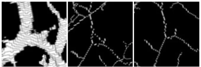
Fig. 2. From left to right: close view of the smoothed image; skele-ton obtained from the smoothed image with the distance-ordered ho-motopic thinning, a loop (i.e. a hole) is clearly visible; skeleton ob-tained after the reconstruction through homotopic growing, no loops are present.
Applying any homotopic thinning algorithm will not yield the desired output, i.e. a set of connected curves that describe the vas-cular tree. Indeed, the thinning of a 3D object (with some endpoint condition) will result in a complex object made of curve or surface patches. We have to adapt the end condition to ensure that the result-ing skeleton is a set of connected curves.
Following [12], we denoted T26(M ) the number of foreground
26-connected components in the 26-neighborhood of M , and T6(M ) the number of foreground 6-connected components in the
18-neighborhood of M . (T26(M ), T6(M )) = (2, 1) characterizes
points M whose deletion will locally divided the foreground into two parts, those points can be considered as curve points. It may however occur that these points are located at thin part of thicker objects (e.g. hourglass) and had more than two 26-neighbors. We defined pure curve pointsas points M verifying (T26(M ), T6(M )) = (2, 1) and
having exactly two 26-neighbors.
A distance-ordered homotopic thinning is performed. Note that the distance map of the homotopic growing can not be re-used since the reconstructed object is slightly different from the smoothed ob-ject. An other distance map is computed inside the reconstructed object. To prevent shrinking, we designed the end condition as fol-lows: when identified, pure curve points are marked as anchor points and are no more considered for further deletion. This ensured that the resulting skeleton is made of pieces of curves.
Tree building. The obtained skeleton is nothing but a binary image which is not convenient for further measurements. A more concise representation is a tree, whose branches and junctions have been recognized. As a final result, the central axis will be stored as a valued tree, with a number of measures attached to either the edges (i.e. the branches) or the nodes (i.e. the junctions).
The skeleton is made of three types of point: • the pure curve points with (T26, T6) = (2, 1),
• the endpoints (that are also simple points) characterized by (T26, T6) = (1, 1), note that they have only one 26-neighbor,
and
• the junction points: these points have three 26-neighbors or more.
The two first point type belongs to vascular branches. The points from these two types are grouped, 26-connected components are
Skeleton Graph n
0
Fig. 3. Left: principle of tree building. Right: a labeled tree built from an image (red: terminal branches; blue: inner branches).
computed which allows to label the branches. Branches that contains one endpoint are terminal branches (except for the root, which is the terminal branch that exhibit the largest attached distance value), while branches without endpoints are delimited by two junctions.
Junctions between branches may be made of several voxels [12]. Again, 26-connected components are extracted but only for junctions points, which enabled to label the junctions between branches. Fig. 3 exemplifies this tree building procedure.
3.2. Quantitative measurements
Vessel branches and junctions have been individualized. Some mea-sures can then be computed:
• for branches: the length, the average diameter;
• for junctions: the lumen area of the parent vessel can be com-pared to those of its children vessel, the angles between the parent vessel and each of its children vessel, or between any two of the children vessels.
Pooling all branches or junctions to compute statistics is by no means relevant since distal branches are obviously of smaller diam-eter than proximal ones. We classified the branches by order, to further compare similar branches. Issued from the quantitative anal-ysis of drainage basins, the Strahler classification, and variants [13], have been already introduced to classify vessel trees. As promoted by Horton [14], the smallest branches (the distal ones) are of small-est order (i.e. 0). Then, the following rules allowed to give an order to all the tree branches:
(i) if all the children branches orders are equal (say of order n), then the parent branch order is n + 1, and
(ii) if the children branches orders are different, the parent branch order is the largest order among its children..
Such a classification is only based on topological considerations and did not take into account geometrical measures (e.g. vessel di-ameter). A more geometrically consistent classification has been proposed [13] that re-classified the tree branches. The principle is that a vessel can be classified as order n + 1 if and only if its average diameter is closer to those of order n+1 than of order n. From a first Strahler classification, the following steps are iterated until stability. 1. The average diameter Dnand the associated standard
devia-tion σnare computed for each vessel order n.
2. Starting from low-order branches, the two above rules applied except that rule (i) is reinforced by the following condition. Let d be the average diameter of the parent vessel, it is of order n + 1 if and only if d > (Dn+σn)+(Dn+1−σn+1)
2
Fig. 4. Diameter-defined Strahler classification of arterial trees.
Fig. 4 displays the classifications of the arterial trees presented in Fig. 1.
Thanks to the classification, we also can compute the connec-tivity matrix T [15] that is defined by Tij =
Nij
Nj where Njis the
number of parents vessels of order j (terminal vessels of order j are ignored) and Nijis the number of children vessel of order i whose
parent vessel is of order j.
4. RESULTS
The different measurements have been pooled by vessel order. Mea-sures related to junctions (comparison of lumen areas, or vessels an-gles) are not presented since they appeared very similar for all the subgroups.
(a) (b) (c)
Fig. 5. From left to right: the number of vessels, the average vessel diameter and the vessel length per vessel order. Blue: wild-type; green: frizzled 6KO; purple: frizzled 4 & 6 KO; red: frizzled 4 KO.
While the average vessel diameter also appeared similar for all the subgroups (see Fig. 5(b)), the vessel lengths and the vessel num-bers (respectively Fig. 5(c) and Fig. 5(a)) suggested an order in the subgroups: wild type, frizzled 6 KO, frizzled 4 & 6 KO and frizzled 4 KO. Surprisingly, the knock-out of the two components frizzled 4 and frizzled 6 appears somehow between the two of them, although it could have been expected that the observed effects of the two of
them will somehow be added. Such findings may help to identify the components that are the more relevant to be further investigated.
Fig. 6. Connectivity matrices for respectively the control, Fzd4 KO, Fzd6 KO, Fzd4 & Fzd6 KO mice.
The connectivity matrices also brought valuable information. For parent vessel up to order 2, the orders of children vessel seem to be split similarly for all subgroups. However, this did not stand any more for parent vessel of order 3 (the largest ones). For wild type mice, parent vessel of order 3 may have children vessels of all orders, while this is not observed for mutant subgroups.
5. CONCLUSION
We have proposed a methodology to analyze and compare vascu-lar trees. This work aims at identifying structural (either geometric or topological) differences between subgroups that may in turn sug-gests hints to understand the importance of the different components involved in a genetic pathway.
The conducted analysis is based on a modified Strahler classifi-cation that takes into account some geometrical characteristics (i.e. the vessel diameter), so as the vessel classes are consistent both geo-metrically (with respect to their average diameter) and topologically (with respect to their proximality in the tree).
The first quantitative results suggest that there might be some structural differences between the subgroups, and that these differ-ences can not be characterized only with geometrical characteristics: e.g. variation of lumen areas at bifurcations or average vessel diam-eter did not appear as discriminant. This emphasizes the need for a quantitative analysis that has to gather both geometric and topologi-cal properties. Obviously, these first results have to be confirmed by a more thorough study that will require to have a sufficient number of individuals in each subgroup, and to quantify the inter-individual variation for a given subgroup. Then, we will have to investigate the influence of the detected morphological difference on the arterial function, and to understand the underlying genetic mechanism that conduct to this structural difference.
A methodological contribution consists in the developed topo-logical tools that ensured to get a thin tree (in the topotopo-logical sense) made of curves for the further analysis. However, it relies on a first segmentation that is nothing but a thresholding. Although some ex-periments demonstrate the stability of the Strahler classification with respect to the threshold choice, some geometrical measures (average diameter, number of branches, branch length) are sensitive to this
choice. In addition, images may exhibit filling defects that also im-pair the segmentation and then the statistical analysis. Therefore, efforts have to be made for a more robust segmentation.
6. REFERENCES
[1] Peter Carmeliet, “Angiogenesis in life, disease and medicine,” Nature, vol. 438, no. 7070, pp. 932–6, December 2005. [2] Napoleone Ferrara and Robert S Kerbel, “Angiogenesis as a
therapeutic target,” Nature, vol. 438, no. 7070, pp. 967–74, December 2005.
[3] Peter Carmeliet and Rakesh K Jain, “Molecular mechanisms and clinical applications of angiogenesis,” Nature, vol. 473, no. 7347, pp. 298–307, May 2011.
[4] Pasquale Cirone, Shengda Lin, Hilary L Griesbach, Yi Zhang, Diane C Slusarski, and Craig M Crews, “A role for planar cell polarity signaling in angiogenesis,” Angiogenesis, vol. 11, no. 4, pp. 347–60, 2008.
[5] B. Descamps, R. Sewduth, N. Ferreira Tojais, B. Jaspard, A. Reynaud, F. Sohet, P. Lacolley, C. Alli`eres, J.M. Lamazi`ere, C. Moreau, P. Dufourcq, T. Couffinhal, and C. Dupl`aa, “Friz-zled 4 regulates arterial network organization through non-canonical wnt/planar cell polarity signaling,” Circ Res, vol. 110, no. 1, pp. 47–58, January 2012.
[6] T Couffinhal, M Silver, L P Zheng, M Kearney, B Witzenbich-ler, and J M Isner, “Mouse model of angiogenesis,” Am J Pathol, vol. 152, no. 6, pp. 1667–79, June 1998.
[7] P. Oses, M.A. Renault, R. Chauvel, L. Leroux, C. Allieres, B. Seguy, J.M. Lamaziere, P. Dufourcq, T. Couffinhal, and C. Duplaa, “Mapping 3-dimensional neovessel organization steps using micro-computed tomography in a murine model of hindlimb ischemia-brief report,” Arterioscler Thromb Vasc Biol, vol. 29, no. 12, pp. 2090–2, December 2009.
[8] Cemil Kirbas and Francis Quek, “A review of vessel extraction techniques and algorithms,” ACM Computing Surveys, vol. 36, no. 2, pp. 81–121, 2004.
[9] Zouina Aktouf, Gilles Bertrand, and Laurent Perroton, “A three-dimensional holes closing algorithm,” Pattern Recogni-tion Letters, vol. 23, no. 1, pp. 523–531, 2002.
[10] Chris J. Pudney, “Distance-ordered homotopic thinning: A skeletonization algorithm for 3d digital images,” Computer Vision and Image Understanding, vol. 72, no. 3, pp. 404–413, December 1998.
[11] G. Bertrand and G. Malandain, “A new characterization of three-dimensional simple points,” Pattern Recognition Letters, vol. 15, no. 2, pp. 169–175, February 1994.
[12] G. Malandain, G. Bertrand, and N. Ayache, “Topological seg-mentation of discrete surfaces,” International Journal of Com-puter Vision, vol. 10, no. 2, pp. 183–197, 1993.
[13] G S Kassab, C A Rider, N J Tang, and Y C Fung, “Morphom-etry of pig coronary arterial trees,” Am J Physiol, vol. 265, no. 1 Pt 2, July 1993.
[14] R.E. Horton, “Erosional development of streams and their drainage basins: hydrophysical approach to quantitative mor-phology,” Bulletin of the Geological Society of America, vol. 56, pp. 275–370, 2008.
[15] W Huang, R T Yen, M McLaurine, and G Bledsoe, “Mor-phometry of the human pulmonary vasculature,” J Appl Phys-iol (1985), vol. 81, no. 5, pp. 2123–33, November 1996.