DIAL • 4, rue d’Enghien • 75010 Paris • Téléphone (33) 01 53 24 14 50 • Fax (33) 01 53 24 14 51 E-mail : dial@dial.prd.fr • Site : www.dial.prd.fr
D
OCUMENT DE
T
RAVAIL
DT/2004/10
Who deserves aid?
Equality of opportunity,
international aid and poverty reduction
Denis COGNEAU
David NAUDET
2
WHO DESERVES AID? EQUALITY OF OPPORTUNITY,
INTERNATIONAL AID AND POVERTY REDUCTION
Denis Cogneau DIAL - UR CIPRÉ de l’IRD
cogneau@dial.prd.fr
Jean-David Naudet
AFD, Département de la Recherche
naudetjd@afd.fr
Document de travail DIAL / Unité de Recherche CIPRÉ
Novembre 2004
ABSTRACT
We build and implement a normative procedure to allocate international aid based on equality of opportunity concerning the risk of poverty. This is an alternative to Collier and Dollar’s proposal (2001) which stresses the impact of aid on worldwide poverty reduction. The big problem with their approach, as regards distributive justice, is that it leaves very great inequality in poverty risk between inhabitants of countries with widely varying structural disadvantages. We draw on post-welfarist theories of social justice, especially those of John Roemer. However our proposal is very different to that of Llavador and Roemer (2001), which has serious methodological errors and reaches contradictory conclusions. Our proposed allocations, like those of Collier and Dollar, differ from current aid allocation by giving more to the poorest countries. Apart from this agreement, our equality of opportunity principle takes account of structural disadvantages to growth rather than quality of past policies. Our kind of allocation shares out poverty risks much more fairly among the world’s population, while reducing global poverty almost as effectively as Collier and Dollar's.
Keywords: International aid, Equality of Opportunity, Poverty Reduction
RÉSUMÉ
Nous élaborons et mettons en œuvre une procédure normative d’allocation de l’aide internationale entre les pays, fondée sur le principe de l’égalité des chances vis-à-vis du risque de pauvreté. Cette procédure constitue une alternative à celle de Collier et Dollar (2001) qui maximise l’impact de l’aide sur la réduction de la pauvreté dans le monde. Du point de vue de la justice distributive, l’allocation de Collier et Dollar présente en effet l’inconvénient majeur de laisser subsister de très larges inégalités de risques de pauvreté entre des individus vivant dans des pays dont les handicaps structurels sont très différents. Notre travail s’inspire des théories « post-welfaristes » de la justice sociale, et en particulier de l’approche de John Roemer. Il fait toutefois une proposition très différente de celle de Llavador et Roemer (2001) qui comporte d’importants défauts de méthode et aboutit selon nous à des résultats contradictoires. Comme les allocations préconisées par Collier et Dollar, les solutions proposées ici diffèrent de la répartition actuelle de l’aide dans le sens où elles privilégient les pays les plus pauvres. Au-delà de ce résultat commun, le principe d’égalité des chances que nous mettons en avant conduit à prendre en compte les handicaps structurels de croissance plutôt que la qualité des politiques passées. Enfin, le type d’allocation que nous proposons égalise beaucoup mieux les risques de pauvreté entre les citoyens du monde, tout en réduisant presque aussi efficacement la pauvreté mondiale que l’allocation de Collier et Dollar.
Mots-clefs: Aide internationale, Egalité des chances, réduction de la pauvreté JEL Codes : F35, I30, D63, O19, O40
3
Contents
INTRODUCTION ... 4
1. AID ALLOCATION AND DISTRIBUTIVE JUSTICE: TWO SEPARATE ISSUES ... 4
1.1. The literature on criteria for allocation aid ... 4
1.2. Overview of post-welfarist theories... 7
1.3. Are theories of justice applicable to international aid? ... 8
1.4. Is Collier and Dollar’s optimal allocation fair? ... 9
2. AID ALLOCATION THAT PROVIDES EQUAL OPPORTUNITIES ... 11
2.1. The problem ... 11
2.2. The allocation process ... 12
2.2.1. A simple definition of poverty risk by 2015... 12
2.2.2. Effort and disadvantage in development of long-term poverty risk ... 13
2.2.3. The minimax criterion of equalizing poverty risk by 2015 ... 14
2.3. Illustration... 15
2.3.1. Calculating parameters ... 15
2.3.2. Calculating optimal allocation... 17
2.3.3. Results ... 17
CONCLUSION... 21
APPENDIX ... 22
BIBLIOGRAPHY ... 25
List of tables
Table 1: Prediction of CPIA by disavantadge variables ... 16Table 2: Optimal allocation variants by equality of opportunity ... 17
Table 3: Correlation between aid allocations and with the variables of disadvantage and apparent effort (CPIA) ... 18
Table 4: Aid allocated ... 18
Table 5: Aid received... 19
Table 6: Projection of poverty and poverty risk inequalities between 1996 and 2015... 21
Table A 1: Aid allocation by country ... 22
4
INTRODUCTION
The allocation of international aid has been very extensively debated for several decades. However, while aid can be seen as wealth redistribution, the contribution of distributive justice theories has barely been considered, except in a recent article by Llavador and Roemer (2001). Since then, the ethical basis of most studies has remained unexplained presupposition.
So the work of Burnside and Dollar (2000) and then Collier and Dollar (2001, 2002) are milestones. They have made a groundbreaking suggestion that aid be allocated to maximise poverty reduction. However, Collier and Dollar’s method is highly debatable in terms of fairness. For example, they would have the Solomon Islands and the Central African Republic receive the same proportion of aid-to-GDP (4.8%). But with the growth equation they estimate and use, the per capita annual growth difference is nearer 5 points (in favour of the Solomon Islands), even if the policies of both countries are just as good. So a poor Centrafrican has far less chance of escaping from poverty by 2015 than a poor Solomon islander. Collier and Dollar’s allocation does not in fact seek equality of opportunity. We take a post-welfarist approach to allocation of international aid. Post-welfarist theories (an extension of Rawls’ work) try to distinguish the separate impact of the efforts and disadvantages of aid beneficiaries. Aid must therefore compensate for the disadvantages while allowing effort to produce “natural reward.” Based on this idea, we shall present a new critical discussion of earlier work done. Then, using the same analytical framework and data as Collier and Dollar, we will devise a way of allocating aid that includes equality of opportunity and compare the results with the optimal allocation obtained by these authors.
Part 1 considers the conceptual basis of existing studies. We show how discussion of international aid allocation has so far considered the issue of desirable allocation. Then we look at post-welfarist theories of justice as they directly apply to our work. After that, we discuss in more detail the relation between equality of opportunity and allocation of development aid. Finally, we analyse Collier and Dollar’s work according to principles of underlying fairness.
Part 2 describes a way to distribute international aid that provides equal opportunity. The basis of it and the problems to be solved are presented, then the various stages of the procedure. Finally the distribution obtained under several hypotheses is discussed and compared with Collier and Dollar’s results.
1. AID ALLOCATION AND DISTRIBUTIVE JUSTICE: TWO SEPARATE ISSUES
1.1.
The literature on criteria for allocation aid1The current debate about optimal allocation of international aid has evolved from three earlier approaches.
For many years, the only criterion considered suitable for giving aid was the level of need. This was usually calculated on the basis of average income or, sometimes, macroeconomic assessment of “gaps” to be made up2. From the groundbreaking work of McKinley and Little (1977, 1978a, 1978b,
1979) to much more recent studies (Berthélemy and Tichit, 2002; McGillivray, 2003b) one major issue has been to define the real determinants of aid allocation and studied the respective influence of the need of beneficiary countries and the motives of donor countries (strategic or commercial, historical ties etc). In a directly normative way, these analyses led to calculating “donor performance”
1 Much has been written on aid allocation and we shall not review it here in detail. A thorough summary was recently done by McGillivray (2003a).
2 All the model-building work done to determine the amount of foreign aid a country requires is part of this vision of need, especially the two gaps model (Chenery and Strout, 1966).
5
(McGillivray and White, 1994) according to how the real share of aid matched need, which was mostly measured by per capita GDP.
In the late 1990s, growing concern about the effectiveness of aid led economists to use another criterion of allocation – the quality of a recipient country’s institutions and policies. The idea that aid is more effective if a country has better economic policies, expounded by Burnside and Dollar (2000) in 1996 and then by others (World Bank, 1998) who added the yardstick of better institutions, has strongly influenced thinking. Nowadays aid cannot be given without its effectiveness being considered. Studies have tried to see whether observed allocation of aid is influenced by the quality of institutions and policies in recipient countries (Alesina and Dollar, 2000; Birdsall, Claessens and Diwan, 2002; Berthélemy and Tichit, 2002; Burnside and Dollar, 2004). They have also sought to once again spell out the donors’ performance requirements according to this new criterion of quality (Dollar and Levine, 2004).
At the same time, an international consensus about making the fight against poverty the main goal of development aid led to another new approach. Few had agreed on how to impartially compare the effectiveness of a set quantity of aid given to two different countries. The amount of poverty it was able to alleviate was one way to do this and make choices. In a series of influential and ground-breaking studies, Collier and Dollar (C&D hereafter) used this new approach to suggest optimal allocation of aid (C&D, 1999, 2001, 2002). Drawing on the previous work of Burnside and Dollar (2000), C&D suggested a growth equation that focused on decreasing marginal effectiveness of aid depending on the quality of institutions and policies3. The level of poverty H is linked to growth G
through an elasticity ε:
∆H/H=-εG=f(initial per capita GDP, region, ICRGE, CPIA, Aid, Aid2, Aid x CPIA) (1)
In a given period, growth determinants are initial per capita GDP, a regional dummy, a measure of institutional quality (the International Country Risk Guide – ICRGE), the World Bank’s Country Policy and Institutional Assessment (CPIA), the ratio of aid to GDP and two quadratic terms – aid over GDP squared and the product of the ratio of aid over GDP with the CPIA. For a given aid package, C&D thus define the level of aid that helps the most people escape from poverty, which means equalising between countries the marginal effectiveness of aid resulting from the equation (1). They express the optimal aid level for a country i with the formula:
a i* = C1 * CPIAi - C2 * (Yi/Hi) * Nib (2)
C1 andC2 andb are positive constants. So optimal aid to a country depends positively on the quality of
its institutions and policies (CPIA) and its poverty level (H) and depends negatively on its per capita income (Y) and its population (N). b is an ad hoc parameter to limit the influence of the population and avoid allocating most aid to only a small number of countries (especially India and China). Compared with the aid disbursed, the optimal allocation calculated by C&D especially favours the poorest countries (high H) implementing the “best” policies (high CPIA). It redirects aid to South Asia, where these two criteria mostly occur together, especially in India and Bangladesh.
C&D’s findings have been expanded on by others (Collier and Dehn, 2001; Collier and Hoeffler, 2002) and, like those of Burnside and Dollar, have been the focus of discussion mostly about the narrowness and fragility of the growth equation used and about its effect on aid allocation (Dalgaard and Hansen, 2000; Dayton-Johnson and Hoddinott, 2001; Hansen and Tarp, 2001; Guillaumont and Chauvet, 2001; Easterly, Levine and Roodman, 2003; Dalgaard, Hansen and Tarp, 2004). Many recent studies on aid effectiveness and allocation have especially looked at the effect of quadratic terms in the growth equation (Roodman, 2003).
As well as policy quality, two of the above studies introduce other variables that can influence the marginal effectiveness of aid. Guillaumont and Chauvet (2001) mention the effect on growth of the
3 This paragraph concerns all the work of Collier and Dollar, whose methods are very similar. The article focuses especially on their 2001 article in World Development.
6
interaction between “aid” and “economic vulnerability”4 and say aid is more effective the higher the
vulnerability. Along the same lines, Collier and Dehn (2001) stress that aid (if well timed) is more effective in the case of strong shocks on export prices. They calculate the adjustments to be made to C&D’s optimal allocation. Daalgard, Hansen and Tarp (2004) test the effect of the interaction between “aid” and “tropical latitude” (considered an indirect structural disadvantage). Their estimates show aid is less effective in the tropics. They thus seriously challenge C&D’s suggested allocation method (see below).
Llavador and Roemer (2001) suggested another basis of aid allocation when they made the first attempt to implement the formal framework of equality of opportunity devised by Roemer (1996, 2000). Our approach is based on this framework too, but our method and findings are very different. Ironically, Llavador and Roemer’s method is a bad illustration of equal opportunity, as it produces results that contradict the principles it claims to be using5.
What is the problem? Llavador and Roemer come up with a growth equation similar to Burnside and Dollar’s, where marginal effectiveness of aid (a) on the growth (G) of a country (i) depends on a variable of macroeconomic performance (inflation, budget deficit, openness), which they regard as a measure of effort (e). The other growth factors are included in a variable of circumstances (C):
Gi = ei (0.959+1.125 ai)+0.095 ai +Ci (3)
They consider donor policy as allocating aid according to policy effort ei and so confine themselves to
seeking an optimal allocation within a family “bei+c” entirely described by the two parameters (b,c).
This choice of feasibility set is due to technical reasons (‘tractability’). However, it very disturbingly endorses an obsession with effort that Roemer also criticises in his theoretical work (see below). Llavador and Roemer then presume that recipient governments choose how much effort (ei) to make
according to how much growth it produces and the (idiosyncratic) disutility of the effort (βi). So effort
ei depends positively on aid received and negatively on βi.
Assuming past aid did not depend on e, they produce estimates of idiosyncratic disutility βi and
(homogenous) marginal disutility η of effort. Then they divide up countries i by their various circumstances Ci and classify them as four types t. So for aid allocation (b,c) it is possible to work out
the effort produced in each quartile of effort q according to each kind of circumstance t: e(q,t,b,c), and the resulting growth G(q,a(q,t,b,c)). Optimal allocation (b*,c*) under equal opportunity is obtained by applying a maximin criterion:
Max Σq γq Min g(q,a(q,t,b,c)) (5)
(b,c) (t)
where γq is the part of the total population in the effort quartile q.
In relation to aid disbursed, Llavador and Roemer produce a very surprising EOp (‘Equality of Opportunities’) allocation. In their sample of 55 countries, East and Southeast Asia receive most (63%) of the $34 billion in available aid compared with 11% of it actually disbursed. Sub-Saharan Africa receives only 3% compared with 41% in reality. South Asia does not figure much because India and Bangladesh are not in the sample. So countries such as South Korea, Indonesia, Malaysia and Thailand, which have the most favourable circumstances, get excessive aid while others (such as Nicaragua and Zambia), which are in the worst-off group, do not get any.
In fact, due to the feasibility limit, which says aid must be clearly linked to effort, and the econometric method used to calculate effort, aid ends up allocated to countries with the best macroeconomic performances (low inflation, small budget deficit, major openness to the outside world). The
4 This last variable is an indicator built around four other variables: the volatility of agricultural value added and export earnings, trends in terms of trade, and the population.
5 It is also not directly comparable with C&D’s allocation. It does not take account of poverty reduction, as it only aims to equalise growth opportunities, and is based on a smaller sample of countries (55 as against 108).
7
correlation between the parameter βi (idiosyncratic disutility of effort) and the allocation obtained is
thus -0.95.
But these countries (in East and Southeast Asia) have also enjoyed better conditions more often, as shown by the correlation between this estimated disutility of effort and the kind of circumstances. So Llavador and Roemer’s allocation will help countries with better past macroeconomic performance, especially those with the highest growth, which are those with best circumstances. The best-off countries get 72% of all aid, compared with 4% going to the worst-off.
We will show how an alternative aid allocation, based on equality of opportunities, can be devised using a more open method that produces more coherent results.
1.2.
Overview of post-welfarist theoriesThe issue of justice in economics has long been restricted to analysing the distribution of individual utilities, which are seen as sufficient for looking at welfare distribution problems. The utilitarian method of maximising aggregate individual utilities has substantially dominated this welfarist approach despite much debate about aggregating preferences. Philosopher John Rawls made the most telling critique of utilitarianism in 1971, which sent welfarism into decline as the dominant theory about economic justice.
Rawls’ theory of “justice as fairness” is mainly a procedural political one based on a social contract between originally free and equal individuals. It challenges welfarism on the grounds that a individual’s freedom cannot be infringed by “aggressive preferences” and replaces the issue of distribution of utilities by one of allocating “primary goods” (a criticism of consequentialism). It further challenges utilitarianism by focusing on the prospects of the worst-off person rather than on maximising overall social welfare. Rawls says inequality resulting from differences in natural advantages and social circumstances is unjust and suggests major principles of fairness to combat them. These include an equal right to an extensive system of liberties, the principle of difference (some inequality is acceptable when it benefits the most disavantaged) and the principle of equal opportunity.
Rawls’ ideas inspired a school of thought sometimes called “post-welfarist,” which expands onthem and in some ways disputes them. Advocates of this egalitarian approach agree about seeking equality in the form of “midfare” (Cohen, 1993), which falls between the supply of resources and achievements in the form of welfare. We are concerned here with two major developments flowing from Rawls’ ideas that deal with compensation and responsibility.
Sen (1980) argued with Rawls about not taking into account people’s different abilities to transform primary goods into welfare. People needing more resources to reach a certain level of welfare have a disadvantage that fair distribution must seek to compensate, but the Rawlsian system does not take that into account (and utilitarianism tends to strengthen such inequality). Dworkin (1981a, 1981b) focuses on the need to define what is and is not the responsibility of individuals. He tries to separate goals (preferences) and assets (resources). Cohen (1989) argued that the true distinction was between responsibility and bad luck. Apart from such differences, these theorists hold that defining the extent of responsibility is vital for devising principles of fairness.
Roemer (1996) crystallised this school of thought in economic terms around the notion of equal opportunity. He stressed that it was difficult to pin down the effects of circumstances and responsibility and advocated equal treatment of individuals in well-defined categories of circumstances (Roemer, 2000).
The common thread of these analyses is an egalitarian approach (based on midfare) and sharing out achievements according to what is due to individual responsibility and what is due to unequal ability and social conditions. The two core principles of the post-welfarist approach are compensation for unjust inequality and that of natural reward that allows differences to arise from the fair result of individual responsibility.
8
Fleurbaey (1996) gave the simplest basic equation for post-welfarism:
yi = f(ti, ei) + xi (6)
where yi is the achievement of an individual i, ti the person’s abilities/disadvantages or circumstances,
ei the degree of personal effort and xi the amount of help (transfers) from social institutions.
A programme of allocating aid according to equality of opportunity must see that it sticks to the principle of equal effort and equal achievement (natural reward) and that of equal ability and equal transfers (compensation).
1.3.
Are theories of justice applicable to international aid?Apart from Llavador and Roemer’s work, theories of justice are strikingly ignored in studies of international aid allocation. Of course, the two kinds of work have been done by a range of authors with different goals and in a variety of contexts: members of a “well-ordered society” (which Rawls describes as constitutional democracy) on the one hand and the international community on the other. However, the aim is similar: to establish principles of justice and efficiency to distribute aid in the best way to beneficiaries in a range of circumstances and with different achievements.
The justice theorists focus on international law and international solidarity (Rawls, 1993) without really elaborating. Sen (1993), who talks of “the myth of big-hearted countries,” warns especially against anthropomorphising countries that automatically elevate individual matters of fairness to national level. He says international redistributive justice is still an issue, but at another level: “The domain of the exercise of fairness involves each nation taken separately…. and the relations between nations are governed by a supplementary exercise involving international equity” (Sen 1999)6.
Llavador and Roemer (2001, op. cit.) also try to justify applying the framework of equal opportunity to international aid.
The post-welfarist approach centres especially on individual responsibility. Can one speak in the same way of a country’s responsibility, of the collective responsibility of its citizens? We do not have an answer but two arguments support looking at aid allocation from a post-welfarist standpoint.
The first is the existence of unjust inequality between countries and thus collectively between their citizens. There are many examples in geography (in terms of isolation, natural resources, climate, and population density), history (epidemics, the slave trade, colonisation) and economics (persistent within country inequalities). These “disadvantages”7 are clearly not the responsibility of present-day citizens
and are a burden on the development of nations and their chances of growth and poverty reduction. It is entirely reasonable to see inequality stemming from these country-specific phenomena as unjust and to try to compensate for them.
The second argument is that the basis of recent discussion of effectiveness and allocation of aid is very close to the post-welfarist starting-point in that it distinguishes two kinds of causes for the performance of developing countries: external variables that have to be accepted (C&D’s regional dummies, for example) and action variables that can be adjusted by reforms (CPIA for C&D). All analysis by supporters of aid selectivity is implicitly based on a developing country’s responsibility for its performance, through the quality of its institutions and policies.
The framework devised by C&D implies quite an arbitrary division between responsibility and disadvantage (‘Dworkin’s cut’). Our aim is not to redefine some sphere of responsibility in development performances but to suggest a post-welfarist interpretation of C&D’s framework and apply in this context an alternative principle of justice in line with equality of opportunity.
6 Sen identifies three kinds of solidarity as three levels of international fairness: “grand universalism” (solidarity between citizens, for example humanitarian aid), “national particularism” (solidarity between nations) and “plural affiliations” (solidarity based on shared identity). We are concerned here with “national particularism.”
7 We define country disadvantage as unjust inequality factors, though talents and social conditions are more often used for these factors where individuals are concerned.
9
The standard post-welfarist framework and allocation of international aid differ in other ways too. These are less fundamental and do not challenge the validity of the approach but they have a conceptual significance and pose special technical problems. We discuss them in the part of the paper about implementing our criteria, but they are worth summarising here.
First, applied post-welfarism is based on gauging talent and social circumstances. Aid is given on the basis of this measurement and should give rise to “natural rewards” for basically unobservable effort. Roemer suggests dividing people into types of observed circumstances and defining effort by quantiles within these types of achievement or advantage variables (Roemer, 2000). In the case of international aid allocation, things are the other way round.
In recent aid literature, geographical and historical disadvantages are not taken into account. Instead, effort is measured through an indicator of the quality of institutions and policies (CPIA for C&D). The problem then is that, according to Roemer (2000), the effort indicator is also influenced by circumstances, because some inbuilt disadvantages affect the quality of policies and institutions. Recent writings about institutions show for example that they are partly determined by geography and long history and that institutions themselves determine the quality of economic policy (Acemoglu et
al., 2001, 2002, 2003). Kaufman and Kraay (2002) point to the difference between a static
measurement of governance and a dynamic one of reform efforts. Where equal opportunity is concerned, an attempt must be made to distinguish pure effort in the total effort observed.
There is also a difference between a person’s own time and a nation’s time. For people, defining “departure and arrival” in equalising opportunity calls for dividing up life-cycles. However this division can be based on major events such as birth, starting school, first job and so on. With countries, as even with overlapping human dynasties, we go from once-off achievements (or utility) by individuals over an objectively limited period of time to achievements over an unlimited period. So we have to arbitrarily fix points of departure and arrival between which equality of opportunity among countries has free rein. The extent of development or poverty at the point of departure contains a great deal of the data about disadvantages and historic effort recorded up to that date.
Handling interaction between aid and other factors in the achievement process (efforts and disadvantages) is a problem. In the simplified version of the post-welfarist equation (6), aid does not interact with the other variables. The key question for post-welfarists is aid/transfer of resources to compensate for a disadvantage without changing anything else. Development aid is on the other hand aid/investment, whose aim is to alter the achievement process and whose interaction with other achievement factors must be considered. These interactions can include aid effectiveness depending on the degree of effort or disadvantage and aid that encourages or does not encourage effort or else reduces disadvantage. In C&D’s growth equation, for example, the interaction of aid and the CPIA is crucial in the aid allocation process.
So the basic post-welfarist model mainly confronts the issue of the fairness of ex-post allocation once individual achievement has been observed. We shall look at the issues of fairness and effectiveness together. The link between aid/investment and the level of associated achievement is more complex due to the interaction of aid with the other variables in the process of producing achievements. This key point is discussed several times below.
1.4.
Is Collier and Dollar’s optimal allocation fair?The theories of fairness enable us to re-examine C&D’s work on aid allocation8.
C&D’s work has helped thinking on the subject to move from a deontological to a consequentialist approach (based on distribution of achievements) in assessing aid allocation. This change is in line with how welfarist theoreticians see things. There was much interest in the motives of donors in the
8 We will not return to a critique of the work of Llavador and Roemer (2001) since it does not deal with the active principle of fairness but with its implementation (see 1.2 above).
10
1970s. Strategic and commercial motives unrelated to a country’s development were disapproved of because it was thought aid had to be disinterested to be fair.
C&D’s approach is an entirely utilitarian one. It determines aid allocation by maximising a function of aggregate social utility where the utility of each person is 0 if the person is below the poverty line and 1 if not. The aggregate utility of the international community is thus set against the total number of poor people. The optimum is achieved when the marginal utility of aid is identical in each country being looked at. The contrast is striking between the influence of C&D’s work in the world of development and the discrediting of purely utilitarian approaches by the theoreticians of fairness. Criticism of utilitarianism naturally applies to C&D’s optimal allocation.
First of all, such allocation is not egalitarian (no attempt is made to equalise an individual or national parameter). The chosen function of collective utility (the number of poor people) gives equal weight to each person. This ignores the fact that such people are not all in the same situation and so do not have the same prospects. With equal effort, the effect of aid is assumed to be equal, meaning that each poor person has the same chance of escaping poverty through aid.
But the overall chances of escaping poverty are heterogeneous and depend especially on “structural” factors, such as which continent a person lives on. A poor African has much less chance than a poor Asian even if their countries have similar policies. A sub-Saharan and a South Asia/Pacific country that are identical (poverty level, governance and so on) will get the same amount of aid under C&D’s allocation. But growth will be very different in each – an average of 4 percentage points higher in the Asia/Pacific country, depending on the regional variables of their growth equation (see also the example in the introduction to this paper). With a poverty/growth elasticity of 2 (C&D’s hypothesis), poverty will fall by an annual 8% more in the Asia/Pacific country, all other things being equal. C&D’s utilitarian allocation is not concerned with equal opportunity.
Aid effectiveness in C&D’s allocation also changes with the CPIA variable, which C&D implicitly regard as to do with reform. Let us suppose the CPIA may or may not depend on the responsibility of the beneficiary countries and their citizens. If the CPIA is not the responsibility of these citizens, we are faced with a familiar perversion of utilitarianism that rewards those in the best circumstances in the name of effectiveness, thus strengthening unjust inequalities.
If we regard the CPIA as the result of collective effort, as C&D seem to do, the most “virtuous” are thereby rewarded. There is a perversion of utilitarianism here too, a more subtle one, that tends naturally towards aid/reward based on merit. Post-welfarists admit the aim should not be to compensate for the consequences of effort, letting “natural reward” arise. They also generally do not think a “social reward” should be added to it, because this would no longer be an egalitarian approach but a definition of fairness as “maximisation of good,” as criticised by Rawls.
Aid/reward raises another familiar problem, the management of time. Applying meritocratic principles involves allocating future resources on the basis of observed past effort. But current aid efforts should determine merit-linked aid. The problem is clear in the case of specific individuals and becomes very worrying when the responsibility of a shifting group of people is involved. This is not commented on by C&D, who allocate future aid on the basis of past CPIA performance. This performance presumably strongly influences future CPIA, for example through a structural parameter of effort disutility expounded by Llavador and Roemer (2001), but this is to admit that the effort observed stems more from disadvantage than pure effort.
Thirdly, C&D put policy quality at the centre of aid effectiveness but do not consider the potential effect of disadvantage on such effectiveness. This point is key for post-welfarists, especially Sen, whose idea of “basic capability” covers exactly this varying ability to convert resources into utility. According to Sen, it depends above all on the talents and disadvantages of individuals as well as their social circumstances. His theory of fairness stresses equalisation of “capabilities.” But C&D do not seem to think aid effectiveness depends on anything other than the quality of institutions and policies
11
of recipient countries, even though they highlight the fact that structural disadvantages are a much greater impediment to growth9.
Their approach can of course take into account differences in poverty/growth elasticity, even if the example they give involves homogenous elasticities of 2. Poverty/growth elasticity is linked to the denominator in the C2 parameter of the equation (2). However C&D’s allocation would give more aid
to countries with greater elasticity, all things being equal, especially countries less badly off. Elasticity differences cover structural disadvantages (initial poverty level and the historically and geographically determined degree of inequality) which aid will worsen rather than compensate for. C&D do not consider the possibility of an inverse link between aid effectiveness and structural disadvantage (climate, historical disruptions, the health of the population, considerable structural inequality). Such a link, if it existed, would clearly show a clash between justice and maximising effectiveness. In terms of the number of people escaping poverty, effectiveness would call for priority aid allocation to poor countries with small disadvantages, which is hard to defend under any notion of fairness.
The theory of a lower yield from aid or investment in countries with historical and geographical disadvantages is a fairly plausible one. It is corroborated by Daalgard, Hansen and Tarp (2004), who point to declining effectiveness of aid in tropical regions. It is also indirectly confirmed by the correlation between the CPIA and some disadvantage variables (see Table 1 in Part 2.3.1). This implication, which hides the efficiency/equity trade-off, perhaps explains the objections to the findings of Burnside and Dollar and then Collier and Dollar. It is not the perfectly good idea that aid has more impact where there are good policies that troubles many analysts, but what is left unsaid – the suggestion that good policy is the only factor that bears on aid effectiveness and should therefore determine aid allocation.
2. AID ALLOCATION THAT PROVIDES EQUAL OPPORTUNITIES
We now suggest a new process for allocating aid that provides equal opportunities, as a basis for criticising the work of Collier and Dollar from the standpoint of fairness.
2.1.
The problemWe start by presenting a basic post-welfarist equation of the kind (6) that links an achievement variable to the functions of the effort and disadvantage factors on the one hand and aid received on the other. The aim of arriving at an alternative sufficiently resembling C&D’s chosen allocation leads us to greatly simplify this very delicate stage. Indeed, it justifies keeping the same basic equation as C&D, their growth equation (1). The problem is then to use it to determine the achievement variable and those of effort and disadvantage.
A first difficulty is choosing the achievement variable. Several are possible, including growth, poverty level and poverty reduction rate. The ex ante nature of development aid (see above) suggests prospects for future achievement as a basis for equal opportunity rather than already observed achievements. This is a serious problem not dealt with by C&D’s static analysis, where future aid is presumed to have an effect under conditions exactly the same as before. The choice and construction of the achievement variable are discussed below, but we have chosen as variable the projected poverty rate in 2015.
Another problem is the distinction between effort and disadvantage (‘Dworkin’s cut’). With C&D’s growth equation, it is quite natural to use the CPIA as an initial measure of apparent effort in recipient countries. In all their analyses, C&D use the CPIA as a yardstick of good management of
9 C&D say sub-Saharan Africa (SSA) has an average governance (CPIA) score of 3.04 and East Asia and the Pacific (EAP) 3.78. If SSA had the same score as the latter (an average ODA/GDP level of 4%), it would gain one percentage point of growth. However, C&D note a 1990-96 growth of –0.8% for SSA and 7.7% for EAP. So the gap between the regions is only marginally explained by quality of governance and almost entirely by “structural disadvantages.”
12
development and CPIA variations as a gauge of commitment to reform. The other factors influencing growth, including initial GDP, then appear as disadvantage factors. But the correlation between the CPIA and some disadvantage factors obliges us to go beyond just measuring apparent effort and to try to find a more exact measure of “pure effort” by aid-recipient countries. Future pure effort will by definition be considered unpredictable. Conversely, the difference between apparent effort (observed CPIA) and pure effort will be structurally part of the disadvantages.
The third problem is handling the interactions between aid and other factors in the achievement process (effort and disadvantages). We have seen that this basic point divides analysis of development aid from the usual post-welfarist analysis framework. Fair allocation of aid must take account of effectiveness. Differential aid effectiveness based on policy quality will enable future aid effectiveness in a country, especially its absorption capacity, to be estimated. C&D duck this issue by suggesting a future CPIA the same as in the past. Predicted CPIA enables us to go a step further. Within the C&D growth equation, the predicted CPIA will be the disadvantage variable influencing the effectiveness of future aid.
A final methodological choice will involve defining the criterion to maximise, determining concretely the allocations that produce the maximum equal opportunity for achievement with equal effort. Again, several solutions are possible (Roemer, 2000; Van de Gaer and al., 2000; Gajdos and Maurin, 2004; Moreno-Ternero, 2004), but we choose for simplicity’s sake the maximin criterion recommended by Roemer.
2.2.
The allocation process2.2.1. A simple definition of poverty risk by 2015
Collier and Dollar consider policy effort both observable and independent of unobservable growth circumstances and say growth in a country i is a (quadratic) function of aid and policy effort, with aid effectiveness depending (positively) on effort:
git = α1 ait - α2 ait² + β eit + γ ait eit + uit (7)
git being average growth of GNP between t-1 and t10,ait aid over GDP and eit observed policy effort in
the same period, and α1, α2, β and γ being parameters, all positive. The remaining more or less
observable factors influencing growth can be grouped in a residual variable uit.
C&D express this growth as a relative variation of poverty through an elasticity εi:
∆Hit /Hit-1 = - εi. git (8)
Hit being the percentage of poor people in the country i at the time t and εi the absolute value of the
poverty/growth elasticity. For C&D, elasticity is presumed constant among countries and over time11.
For the average representative agent of the country i, at the end of the period T (for example in 2015) during which levels of aid and effort (and elasticity) will be kept constant, the ex ante risk of poverty appears as a function of aid received over the period, of policy effort and the initial poverty rate: HiT (ai,ei) = Hi0 [1 – εi.( α1 ai - α2 ai² + β ei + γ ai ei + ui)]T (9)
where ui is growth prospects independent of aid and policy effort, that an international planner must
use to predict changes in poverty under various aid scenarios.
We define poverty risk, HiT(ai,ei), as the achievement variable from which we want to assess equality
of opportunity between representative people in each country. As Roemer points out, the achievement
10 Standard estimates are for five-year periods.
11 C&D use an elasticity of 2. It may seem unrealistic to assume poverty elasticity is homogenous. Bourguignon (2002) in particular shows that under a log-normal revenue distribution hypothesis, such elasticity depends negatively on the level of initial poverty (Hi0) and initial income inequality (the Gini indicator for example). We discuss later on an extension of our application introducing a heterogeneous elasticity εi(Hi0,Gini0).
13
variable is chosen mainly for non-economic reasons. Llavador and Roemer (2001), for example, just choose growth and point out that per capita GDP and the level of poverty or child mortality could also have been used as variables.
We could also have used the relative risk reduction -∆HiT /Hi0. This advantage variable would then
only involve growth (aid, effort and circumstances) as in Llavador and Roemer application. We would also try to equalise chances of escaping poverty between individuals present in both t=0 and t=T and who were poor in t=0. We could then allocate a lot of aid to a country with initially few poor people but whose growth prospects were especially bad, as in some former Soviet Bloc countries. In view of the millennium development goals, we could also have kept the distance between initial poverty (target poverty level) and the actual level of it: (Hi0/2)-HiT=-(Hi0/2)-∆HiT. Again, the criterion
would tend to minimise differences in the initial poverty level, although less so than before. 2.2.2. Effort and disadvantage in development of long-term poverty risk
The achievement variable we have chosen, HiT(ai,ei), shows that every inhabitant of the world at the
date T does not have the same chance of being poor, not just because of efforts made ei but also
because of other growth factors ui, poverty/growth elasticity εi, and initial poverty Hi0. These three
factors are theoretically beyond the responsibility of countries during the period [0; T], so we will call them “disadvantage variables”.
These variables may also affect observed effort during the period [0; T]. The international planner must not only get an idea of growth prospects ui, but also of the amount of policy effort made. To
apply the equal opportunity variable properly, we must distinguish, within the ex ante effort, the proportion of predictable disadvantage and of pure effort, as free expression of policy responsibility (‘Dworkin’s cut’). Like C&D, but unlike Llavador and Roemer, we suggest that each country’s pure effort is independent of the amount of aid it gets. There is no motivational restraint linked to aid distribution. Aid does not discourage effort, any more than it encourages it12. Suppose ex ante effort
is expressed as a sum of two independent elements, pure effort Ei, withzero expectation and a function
e of disadvantage variables:
ei = Ei + e(Hi0,ui,εi) (10)
We show in Table 1 in part 2.3.1 that C&D’s effort variable (the CPIA) depends significantly on disadvantage variables. We then see that, in C&D’s chosen framework, aid effectiveness over growth, through parameter γ, depends not only on pure effort but also on disadvantage13. As C&D did not
consider this possibility, their optimal allocation is based on taking into account efforts that include circumstances. By giving more aid to countries that show greater “apparent effort,” they more often (if δe/δH is <0 and δe/δu is <0) give aid to countries that have good circumstances. These circumstances help aid to effectively reduce poverty but they mean C&D’s optimal allocation is further from an equal opportunity allocation.
Let us assume êi=ê(Hi0,ui,εi) is expected effort arising from disadvantage variables. In the absence of
aid, the difference in poverty risk by the date T now depends only on the initial poverty level, growth disadvantages and poverty/growth elasticity – in other words factors that are beyond the (present and future) responsibility of the country. If:
hiT = Hi01/T [1 – εi.(β.êi + ui )] (11)
12 Llavador and Roemer (2001) use the latter hypothesis while Knack (2003) uses an opposite one to show a negative correlation between progress in governance measured by variations in the ICRGE indicator and aid received.
13 Econometrically, the coefficients α1, α2 and especially γ obtained by C&D are thus biased, in particular γ is overestimated because of the positive correlation between effort and favourable circumstances. If however a measurement error is introduced into effort (say, in an additive form: ei = Ei + ρ ui + ηi), then the sign of bias on the coefficients becomes indeterminate. In the application, we ignore these problems and use C&D’s coefficients.
14
hiTT is the ex ante prospects for poverty in country i at the date T, if they get no aid and if they make a
policy effort which is predictable on the basis of their disadvantage variables during the whole period between 0 and T. The ex ante poverty risk by the year T having received aid ai and having made pure
effort Ei can be expressed as:
HiT (ai, Ei) = [ hiT - Hi01/T εi.(α1 ai - α2 ai²+ γ êi.ai + γ Ei.ai ) ] T (12)
Our criterion will be to equalise differences of poverty risk by the date T between countries facing different disadvantages but making the same degree of effort. The inclusion of a more distant date (larger T) gives more weight to growth prospects and possible differences in elasticity, in relation to the amount of initial poverty, since the two terms in Hi0 in (11) and (12) are raised to the exponent 1/T.
The expression (12) also shows that the effectiveness of aid in reducing poverty potentially depends on all the disadvantage variables considered.
Under Sen’s notion of “capability,” the capacity to transform the resource (aid) into achievement (poverty reduction) varies widely. The formula says first that aid received compensates disadvantages in poverty prospects better when initial poverty is greater. So since aid does not by assumption target
the poor, the growth it generates concerns them more if poverty is more widespread14. Second,
aid-driven growth is better transformed into poverty reduction when elasticity is higher. Lastly, the effectiveness of aid in boosting growth depends on disadvantage variables grouped here in the term êi = ê(Hi0,ui,εi) and also, in line with Burnside and Dollar’s original notion, accepted by C&D, on a
pure policy effort Ei. Since aid has to be allocated ex ante, before any special circumstances
(uiT instead of de ui) or effort (ei instead of êi) arise, the only valid prediction of pure effort is the
expectation of it, that is, 0:
E(HiT|ai ,Hi0,ui,εi) = HiT (ai, 0) = [ hiT - Hi01/T εi.(α1 ai - α2 ai²+ γ êi.ai) ] T (13)
This point in our approach is key. C&D, along with Llavador and Roemer, use data from past efforts to calculate their optimal allocations (see Part 1.1). Conversely, we have declined to predict a country’s pure effort. We could have used Êi= ei -êi to do so, considering that the difference between
observed and predicted effort reflects a structural national propensity to make a policy effort that will amount to collective responsibility. This option does not seem ethically justifiable to us. But it would not anyway change the principle of our method. We would have to allow the natural reward linked to such effort to come into play, while still refusing to add a “merit” -based social reward. We have verified that this kind of variant does not change the results of our illustration (see also note 15). 2.2.3. The minimax criterion of equalizing poverty risk by 2015
To apply a criterion of equal opportunity, we argue that the “international planner” must only try to predict a country’s growth differential ui. The equal poverty risk principle leads to aid allocation to
minimise poverty level differences by the date T. The optimal allocation (ai*) is sought,
corresponding to Rawls’ minimax system:
Min Max { [ hiT - Hi01/T εi.(α1 ai - α2 ai² +γ êi.ai) ] T }
u.t.c. Σ ai yi0 = A0 (14)
0 < ai
Budget restraints involve allocating aid for the period 0 within an aid total A0. Over time, this total
varies with changes in national GDP yit. Donors are assumed to commit to this optimal allocation (ai*)
throughout the period T and accept changes over time in the total that their commitment involves (C&D make the same argument).
15
The choice of Rawls’ minimax criterion again calls for non-economic arguments. Very broadly, we could try to minimise any inequality index between poverty risks (Moreno-Ternero, 2004). The algorithmic answer to the problem would be more complex and might include multiple solutions. The criterion also only allows a solution if the poverty risk is always decreasing in ai. The convexity
of the relationship (positive α1 and α2) means there is maximal aid amaxi = (α1+γêi)/2α2 such that any
more than this will not be efficiently absorbed and will hinder growth. Even with maximal aid amaxi,
the country with the worst poverty prospects in 2015 may not rise to the level of the second poorest country. A saturation effect limits the possibilities of aid as a means of equalising opportunity. So the minimax criterion has to be defined more precisely, in the following way:
Min Max{ [ hiT - Hi01/T εi.(α1 ai - α2 ai² +γ êi.ai) ] T | i such that ai < amaxi }
u.t.c. Σ ai yi0 = A0 (15)
0 ≤ ai ≤ amaxi
As long as the country with maximum disadvantage gets less than maximum aid amaxi, the country
will remain part of minimisation. If it needs to be given amaxi to minimise the criterion, since it
cannot be given more, it gets excluded from the programme and is said to be “saturated.” The optimal allocation (ai*) then comprises countries with the biggest disadvantages and which get amaxi because
they are saturated and less disadvantaged countries get less aid than amaxi and have equalised poverty
risk. The first group of countries have heterogeneous poverty risks that are all higher to the homogeneous risks of the second group, but aid cannot help them further15.
2.3.
Illustration2.3.1. Calculating parameters
Like C&D, we start from 1996 (T=0) and take 2015 as the goal, which means T=20. We use the same country database as C&D (2001), comprising 108 countries receiving aid in 1996. In that year, the total aid available A0 ($71 billion) was the same as the total used by C&D to calculate their optimal
allocation16. The countries’ GDPs are at 1996 purchasing power parity. Like C&D, the poverty line
used is $2 per capita a day. Initial poverty rates Hi0 are also the same as C&D’s. Parameters α1, α2, β
and γ are estimates C&D use to calculate aid allocation (α1=0, α2=0.04, β=0.64, and γ =0.18).
Apparent effort levels are measured by CPIA categories numbered 1 to 5 by C&D17. To calculate
factor êi, we regress the CPIA scores over two disadvantage components – the regional indicators for
growth prospects and the initial poverty level. We use the value predicted by the regression.
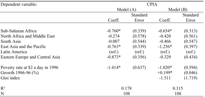
As Table 1 shows, at a given level of poverty, the 1996 CPIA was markedly less in sub-Saharan Africa, East Asia and the transition countries than elsewhere. Regardless of region, the poorest countries also got the worst scores. As Dalgaard, Hansen and Tarp (2004) noted, the CPIA is also strongly tied to previous growth performances (which serve to predict growth prospects in one of the proposed variants).
Poverty/growth elasticity εi is assumed identical at 2, following C&D. To predict growth prospects ui,
we first use regional growth differences estimated by C&D, which are the coefficients of the regional dummies in South and East Asia, sub-Saharan Africa, the Middle East and North Africa, Eastern Europe and Central Asia, and Latin America. We also take account of growth differences caused by
15 In the above example, where a heterogeneous pure effort Êi is taken into account, the maximin criteria will be changed in the following way: Min ΣE Max [ hiT - Hi01/T εi.(α1 ai - α2 ai² + γ êi.ai + γ Êi.ai ) ] T in line with Roemer (2000).
16 As C&D note, the total aid for the 108 countries is only $38 billion, not $71 billion. In their paper, C&D give no clue about their use of the larger figure to calculate their optimal allocation. As we want to be able to compare our allocation with theirs, we use the same amount as they do. Comparison with the observed 1996 allocation thus becomes less appropriate.
17 Unlike C&D, we do not have true CPIA levels because such data was not published by the World Bank. By numbering the CPIA categories 1 to 5, the marginal effectiveness of reconstituted aid is thus not quite the same as C&D’s. But this difference is very small and less important.
16
predicted effort êi (in the term β.êi)18. We set these differences around an average 1% per capita GDP
growth for 1996-201519. Based on 1996 poverty levels, growth prospects and estimates of predicted
effort, we can then calculate poverty prospects in 2015 with zero aid: hiT T = Hi0 [1 – 2.(β.êi + ui )]T.
Table 1: Prediction of CPIA by disavantadge variables
Dependent variable: CPIA
Model (A) Model (B) Coeff. Standard Error Coeff. Standard Error
Sub-Saharan Africa -0.760* (0.339) -0.654* (0.313)
North Africa and Middle East -0.274 (0.578) -0.420 (0.561)
South Asia -0.007 (0.544) -0.466 (0.547)
East Asia and the Pacific -0.763* (0.339) -1.256* (0.397)
Latin America (ref.) (ref.) (ref.) (ref.)
Eastern Europe and Central Asia -0.873* (0.356) -0.329 (0.434) Poverty rate at $2 a day in 1996 -1.414* (0.637) -1.020* (0.594)
Growth 1986-96 (%) +0.199* (0.046)
Gini index -1.511 (1.719)
R² 0.178 0.315
N 108 108
Method: Ordinary least squares*: significant at 10%
We then make two variants on disadvantage variables to see how sensitive our allocation is to two sources of heterogeneity in the countries – one to do with poverty/growth elasticity and the other to do with growth prospects.
Taking account of differential elasticity is interesting because it directly ties in with Sen’s notion of “capability”, describing the capacity to convert a resource (in this case, aid) into achievements (poverty reduction) as explained earlier. Drawing on Bourguignon (2002), we reconstitute theoretical poverty/growth elasticity for 1996 and 2015, assuming log-normality of income distribution. In 1996, these elasticities are based solely on C&D’s 1996 $2 poverty rates. Taking into account the Gini indexes available for the 1990s20, we then calculate a purchasing power parity per capita GDP
adjustment factor to determine these poverty levels from the theoretical formula arising from log-normal distribution.
Assuming that this adjustment factor and Gini indexes are fixed, we calculate theoretical elasticity in 2015 from predicted 2015 per capita GDP based on 1996-2015 growth prospects. The 1996-2015 growth is involved because elasticity changes with per capita GDP21. Finally we use the average of
the 1996 and 2015 theoretical elasticities. This average depends negatively on 1996 poverty levels, negatively on Gini-measured initial inequality levels and positively on growth prospects. This formula shows more than 80% of countries with elasticity below 2, with a minimum of 0.03 and a maximum of 3.51.
We then look at a second variant which introduces heterogeneity in growth prospects in each region. From average annual growth rates in these countries between 1986 and 1996, we calculate for each country how far its growth deviates the regional average and add this difference to the growth prospects used initially for 1996-2015.
18 So growth prospects are not strictly homogeneous within regions since the predicted effort also depends on the rate of initial poverty, as shown in Table 1.
19 Our first concern is not the realism of growth prospects. Table 5 however shows that we obtain credible figures for poverty changes between 1996 and 2015.
20 The 6-point correction suggested by Deininger and Squire is applied for the Gini indexes based on income and not consumption data. When unavailable, the Gini index is presumed equal to the regional average.
17
Table 2: Optimal allocation variants by equality of opportunity
Allocations Elasticity (εi) Growth prospects (ui)
EOp1 2 1% + C&D regional deviation + (deviation from predicted effort) EOp2 εi=ε(Hi0,Gini0,ui) 1% + C&D regional deviation + (deviation from predicted effort)
EOp3 εi=ε(Hi0,Gini0,ui) 1% + C&D regional deviation + (deviation from predicted effort) + deviation
from 1986-96 growth
Hi0= initial poverty rate at $2 (1996); Gini0= Gini index of initial income inequality(1990s).
For allocations EOp1 and EOp2, effort is predicted using the model (A) in Table 1 and for EOp3 model (B). 2.3.2. Calculating optimal allocation
So the proposal for equalising opportunity through international aid consists of minimising the maximum 2015 poverty risk (based on the 108 countries). The algorithm divides up the countries by risk of poverty with zero aid (hiT). It then calculates for each country the amount of aid needed to lift
the country i and all the countries at greater disadvantage to the 2015 poverty risk level of the next poorest country (i+1). This requires solving a second-degree equation and giving it the smallest positive root.
However, the equation may be unsolvable because aid becomes ineffective above a certain level. A makeshift solution must be found, as explained above. The aid amount used is then amaxi, the level at
which the marginal effectiveness becomes zero and the country receives no more extra aid during the allocation algorithm. It is said to be “saturated”22. So aid is allocated to countries bit by bit until the
fixed total of aid is reached.
When the aid needed to lift the country and its non-saturated predecessors to the level of the next country exceeds this fixed total, the allocation process described above ceases to operate. The country in question is called the “pivotal country.” The algorithm then calculates how much aid is left over and allocates it to the “pivotal country” and its non-saturated predecessors so as to lessen further their poverty risk and reach the exact figure of the available fixed aid. All countries better off than the “pivotal country” will not get any aid. Their 2015 poverty risk is anyway lower than countries in the same effort category that get positive aid.
2.3.3. Results
Table A1 in the Appendix shows detailed country results for each simulated allocation. Table 3 synthesises international aid allocations according to the equality of opportunity we have devised, through a correlation matrix. The EOp1 and EOp2 allocations are very closely correlated. They share growth prospects and differ only in their national poverty/growth elasticity. As expected, the EOp3 allocation is further from the other two, especially the first one. This first result shows the key role of growth prospects, which strongly influence a country’s disadvantages, either directly or through changing elasticity over time.
The three allocations are also positively correlated to C&D’s allocation. And although the comparison is less valid because it does not involve the same single amount of total aid, the three allocations, according to equal opportunity, correlate similarly to the effective 1996 allocation. They are also much further from it than C&D’s allocation is.
The correlation of the three allocations with the 1996 poverty level is high – equal or higher to C&D’s. The latter arbitrates between this initial poverty level and the apparent policy effort measured by the CPIA, while the EOp allocations arbitrate between poverty and prospects for growth. So they more
22 This maximal aid amount in percentage of GDP varies according to predicted CPIA, so according to initial poverty level and regional dummies. For the EOp1 and EOp2 scenarios with model A in Table 1, it lies between 5.5 and 9.8% (average 7.5%). For the EOp3 variant and with model B, it is between 3.8 and 11.0% (also an average 7.5%).
18
often favour countries that get a bad CPIA score, in view of the CPIA’s (negative) correlations23 with
poverty and with growth prospects (positive, mainly with EOp3).
Table 3: Correlation between aid allocations and with the variables of disadvantage and apparent effort (CPIA)
EOp1 EOp2 EOp3 C&D 1996 aid
EOp1 1.0 0.89 0.80 0.58 0.48 EOp2 1.0 0.65 0.55 0.47 EOp3 1.0 0.55 0.43 C&D 1.0 0.70 $2 poverty (1996) 0.72 0.75 0.69 0.69 0.52 Growth1 -0.68 -0.56 -0.46 -0.30 -0.29 Growth2 -0.37 -0.39 -0.53 -0.23 -0.24 Gini indicator 0.48 0.44 0.25 0.25 0.23 CPIA -0.33 -0.32 -0.35 -0.16 -0.25
Key: The Pearson coefficient of correlation is between the horizontal and vertical variable. The vertical shows aid allocation as percentage
of GDP. EOpx: see Table 2; C&D: Collier and Dollar’s allocation; 1996 aid: effective allocation; Growth1: growth prospects used for EOp1 and EOp2; Growth2: growth prospects used for EOp3.
Table 4 summarises the result of allocation by major regions and this time shows a big difference between the EOp1 allocation on the one hand and its two heterogeneously elastic variants and the C&D allocation on the other. In the first case, no aid has been allocated to South Asia, which allows sub-Saharan Africa and, secondarily, Latin America and East and Central Asia, to get more. Bangladesh, India and Nepal have initial poverty levels just as high as the poorest African countries but have much better growth prospects, which would suggest substantial poverty reduction between 1996 and 2015 if the poverty/growth elasticity is 2 (as C&D also suppose). Where elasticity is more realistic24, poor South Asian countries get significant and even more aid than the amount
recommended by C&D.
This similarity between the EOp2 and EOp3 allocations and that of C&D is misguiding however. First, aid allocated to India is limited ad hoc in C&D’s model through a population parameter that restricts the possibility of giving aid to a single country (see 1.1, equation (2)). We introduce no such limitation. Also, the smaller weight of sub-Saharan Africa in EOp2 and EOp3 is because South Africa gets no aid (see Table A1), while its GDP is a third of Africa’s total. The country has a 50% poverty rate and average growth prospects and is thus rivalled by poorer South Asian countries (India, Bangladesh and Nepal, which have over 80% poverty).
EOp2 and EOp3 allocations are more generous to the poorest countries in Latin America and the Caribbean, Eastern Europe and Central Asia, to the detriment of those in East Asia whose growth prospects are good and which reward C&D’s allocation, such as Laos, Vietnam, Mongolia and Papua New Guinea (see Table A1).
Table 4: Aid allocated
EOp1 EOp2 EOp3 C&D
Sub-Saharan Africa 4.5 2.7 2.3 3.3
North Africa and Middle East 0.0 0.0 0.0 0.0
South Asia 0.0 1.9 2.0 1.5
East Asia and Pacific 0.0 0.0 0.0 0.1
Latin America 0.6 0.2 0.2 0.1
Eastern Europe and Central Asia 0.7 0.3 0.4 0.1
Note: Percentage of regional GDP (PPP 1996).
23 This negative relationship between the poverty rate and the CPIA also explains why C&D’s allocation is (slightly) negatively correlated with the CPIA.
19
Table 5: Aid received
EOp1 EOp2 EOp3 C&D Aid 1996
Sub-Saharan Africa 53.6 31.8 27.2 39.5 38.2
North Africa and Middle East 0.0 0.0 0.0 0.0 9.9
South Asia 0.0 51.3 53.5 41.5 12.9
East Asia and Pacific 0.0 0.0 0.0 8.5 17.6
Latin America 26.0 9.4 8.4 6.6 12.9
Eastern Europe and Central Asia 20.3 7.4 10.9 3.9 8.5 Note: Percentage of total aid.
The main differences between the EOp and C&D allocations can be summed up by regressing the difference between aid (in relation to GDP) in the cases of EOpx and C&D over the relevant characteristics of the countries for each allocation – initial poverty, Gini indicator, per capita GDP, population, growth differences and apparent policy effort (CPIA). These variables are the ones involved in calculating an allocation. The results of this multivariate analysis go with those in Table 3 and are given in Table A2 in the Appendix. The linear regressions made explain in each of the three cases at least half of the variance of differences (as much as 65% of the variance of differences between EOp1 and C&D)25. They show that what likens or differentiates the two kinds of allocations
is the principle of fairness that has guided their compilation.
So the EOp and C&D allocations are similar in taking the poverty level into account. However, at a given poverty level, growth prospects in the EOp allocations, and the CPIA, per capita GDP and population in the C&D one are the variables that explain the difference. The EOp allocations compensate countries with poor growth prospects at a given effort and poverty level. The C&D allocation helps countries that score well in apparent policy effort (CPIA) and also low per capita GDP countries with small population, also at a given poverty level. This advantage enjoyed by poorer and smaller countries in the C&D allocation has already been noted (see equation (2), 1.1). It arises from the combination of three factors: (i) the effectiveness of the marginal aid dollar is higher in countries with low overall GDP, (ii) the C&D criterion seeks to maximise the number of poor people who have escaped from poverty, and (iii) C&D introduce an ad hoc limitation of the population factor so as not to allocate all aid to India.
So the allocations suggested here contrast, like C&D’s, with the present distribution of aid by giving more weight to the poorest countries. Apart from this general result, the principle of equal opportunity leads to several possible allocations since it calls for a prediction. In line with C&D’s main result, an allocation according to equal opportunity could very well call for redirecting a large part of international aid (about a third in the case of EOp2, EOp3 and C&D) to South Asia, where poverty is as high as in sub-Saharan Africa.
But this similar conclusion does not arise from the same principles at all. For C&D, Bangladesh, India and Sri Lanka are both compensated for their high poverty level and rewarded for their high score for quality of institutions and policy, which is supposed to correspond to their past efforts. With our EOp allocations, only their poverty level and independent growth prospects are involved. As soon as these growth prospects are good enough to hope for substantial poverty reduction by 2015 without aid or special policy efforts, aid should be redirected to other regions with less bright futures.
This is the rationale of the EOp1 allocation, where poverty/growth elasticity of 2 produces very significant poverty reduction in the Indian sub-continent by 2015 (see Table 6 below) and thus the region’s exit from the group of countries most deserving of international aid. This allocation, based only on the regional growth differences obtained by C&D and which uses the same elasticity assumption, is also the closest methodologically to the C&D allocation. It significantly produces the most opposite results in regional aid allocation, redirecting 15% of aid to Africa, 15% to Latin
25 The variables taken into account are the only ones involved in compiling the allocations, so the difference between them is a very complex but accurate non-linear function of these variables. The linear regressions are only an approximation of it reflected by the R² of the regressions (percentage of explained variance).