Comparison of CFD predictions of the forces and flow patterns with experiments data for an escort tug model with yaw angle

(1)

Publisher’s version / Version de l'éditeur:

https://publications-cnrc.canada.ca/fra/droits

L’accès à ce site Web et l’utilisation de son contenu sont assujettis aux conditions présentées dans le site LISEZ CES CONDITIONS ATTENTIVEMENT AVANT D’UTILISER CE SITE WEB.

Technical Report (National Research Council of Canada. Institute for Ocean Technology); no. TR-2006-22, 2006

READ THESE TERMS AND CONDITIONS CAREFULLY BEFORE USING THIS WEBSITE.

https://nrc-publications.canada.ca/eng/copyright

NRC Publications Archive Record / Notice des Archives des publications du CNRC :

https://nrc-publications.canada.ca/eng/view/object/?id=2f33f094-a481-48d1-b337-24a9d9256cf4 https://publications-cnrc.canada.ca/fra/voir/objet/?id=2f33f094-a481-48d1-b337-24a9d9256cf4

Archives des publications du CNRC

For the publisher’s version, please access the DOI link below./ Pour consulter la version de l’éditeur, utilisez le lien DOI ci-dessous.

https://doi.org/10.4224/8894853

Access and use of this website and the material on it are subject to the Terms and Conditions set forth at

Comparison of CFD predictions of the forces and flow patterns with experiments data for an escort tug model with yaw angle

(2)

REPORT NUMBER TR-2006-22

NRC REPORT NUMBER DATE

September 2006 REPORT SECURITY CLASSIFICATION

Unclassified

DISTRIBUTION Unlimited TITLE

COMPARISON OF CFD PREDICTIONS OF THE FORCES AND FLOW PATTERNS WITH EXPERIMENT DATA FOR AN ESCORT TUG MODEL WITH YAW ANGLE

AUTHOR(S)

David Molyneux

CORPORATE AUTHOR(S)/PERFORMING AGENCY(S)

Institute for Ocean Technology, National Research Council, St. John’s, NL PUBLICATION

SPONSORING AGENCY(S)

Institute for Ocean Technology, National Research Council, St. John’s, NL IOT PROJECT NUMBER

42_2072_10

NRC FILE NUMBER

KEY WORDS

Hydrodynamic, escort tug, CFD, yaw angles

PAGES v, 39 FIGS. 38 TABLES 21 SUMMARY

This report describes the development of CFD predictions for the forces and flow patterns for an escort tug at typical operating angles to the flow and the comparison of these predictions with data from model experiments. Some conclusions are made on the effectiveness of commercial RANS based CFD codes within the design process for ship hulls that are required to operate at large yaw angles. In the case of an escort tug this angle can be up to 45 degrees.

ADDRESS National Research Council Institute for Ocean Technology Arctic Avenue, P. O. Box 12093 St. John's, NL A1B 3T5

(3)

Institute for Ocean Institut des technologies

Technology océaniques

COMPARISON OF CFD PREDICTIONS OF THE FORCES AND

FLOW PATTERNS WITH EXPERIMENT DATA FOR AN

ESCORT TUG MODEL WITH YAW ANGLE

TR-2006-22

David Molyneux September 2006

(4)

TABLES OF CONTENTS

List of Figures ... iv

List of Tables... v

INTRODUCTION ... 1

MODEL EXPERIMENTS TO MEASURE HYDRODYNAMIC FORCES ... 3

CFD PREDICTIONS OF HYDRODYNAMIC FORCES ... 6

Domain Dimensions... 6

Tetrahedral Mesh ... 6

Hexhedral Mesh ... 9

CFD Solver ... 11

COMPARISON OF CFD PREDICTIONS WITH EXPERIMENT DATA FOR... 13

FORCE COEFFICIENTS AT OPERATING YAW ANGLES... 13

Hull Only ... 13

Hull & Fin ... 15

CFD PREDICTIONS OF FLOW PATTERNS AT 45 DEGREES YAW ... 17

COMPARISON OF FLOW PATTERNS FROM CFD SIMULATIONS WITH RESULTS OF PIV EXPERIMENTS ... 22

Upstream, No Fin... 26

Downstream, No Fin... 26

Downstream, With Fin... 26

NUMERICAL ANALYSIS OF FLOW PATTERNS PREDICTED BY CFD AGAINST MEASURED PIV DATA ... 26

Upstream side, no fin, tetrahedral mesh... 28

Upstream side, no fin, hexahedral mesh ... 29

Down stream side, no fin, tetrahedral mesh... 30

Down stream side, no fin, hexahedral mesh ... 31

Down stream side, with fin, tetrahedral mesh... 32

Down stream side, with fin, hexahedral mesh ... 33

Through plane velocity components... 34

In-plane velocity components ... 34

RECOMMENDATIONS FOR FURTHER STUDY... 37

CONCLUSIONS... 37

ACKNOWLEDGEMENTS... 38

(5)

LIST OF FIGURES

Figure 1, Body plan for escort tug ... 2

Figure 2, Side view of escort tug, showing low aspect ratio ... 2

Figure 3, Model tested on PMM (10 knots)... 4

Figure 4, Force coefficients for an escort tug hull with different appendages for a flow speed of 0.728 m/s ... 5

Figure 5, Scope of mesh (shown for tetrahedral mesh and tug with fin)... 7

Figure 6, Tetrahedral mesh for escort tug, with fin, waterline view... 8

Figure 7, Tetrahedral mesh at midship section ... 8

Figure 8, Tetrahedral mesh for escort tug, profile view ... 9

Figure 9, Hexahedral mesh for escort tug, waterline view ... 10

Figure 10, Hexahedral mesh at midship section ... 10

Figure 11, Hexahedral mesh for escort tug, profile view ... 11

Figure 12, Comparison of CFD predictions for force coefficients with experiment values, hull only ... 14

Figure 13, Comparison of CFD predictions for force coefficients with experiment values, hull and fin ... 14

Figure 14, Planes used for comparing predicted flow patterns with PIV measurements . 18 Figure 15, Flow vectors for tetrahedral mesh ... 19

Figure 16, Flow vectors for hexahedral mesh... 19

Figure 17, Flow vectors for tetrahedral mesh ... 20

Figure 19, Flow vectors for tetrahedral mesh ... 21

Figure 21, In-plane vector comparisons, upstream side without fin, tetrahedral mesh .... 23

Figure 22, In-plane vector comparisons, upstream side without fin, hexahedral mesh.... 23

Figure 23, In-plane vector comparisons, downstream side without fin, tetrahedral mesh 24 Figure 24, In-plane vector comparisons, downstream side without fin, hexahedral mesh24 Figure 25, In-plane vector comparisons, downstream side with fin, tetrahedral mesh .... 25

Figure 26, In-plane vector comparisons, downstream side with fin, hexahedral mesh .... 25

Figure 27, In-plane error, magnitude and direction ... 28

Figure 28, Through plane error, magnitude ... 28

(6)

LIST OF TABLES

Table 1, Summary of principle particulars for escort tug ... 3

Table 2, Summary of overall domain dimensions ... 6

Table 3, Summary of mesh dimensions... 7

Table 4, Parameters for κ−ω turbulence model... 12

Table 5, Comparison of CFD predictions for hydrodynamic forces, tug with no fin... 13

Table 6, Comparison of CFD predictions for hydrodynamic forces, tug with fin... 15

Table 7, Comparison of pressure and viscous forces acting on tug and fin (hexahedral mesh)... 16

Table 8, Renamed axis system between CFD simulations and PIV experiments ... 22

Table 9, Shift of origin in PIV measurements ... 22

Table 10, Summary of error in CFD prediction... 28

Table 16, Non-dimensional values of Erroru... 34

Table 17, Non-dimensional mean, Error2D... 35

Table 18, Non-dimensional standard deviation, Error2D... 35

Table 19, Fraction of data set where Error2D was within ... 35

Table 20, Comparison between Series 60 and escort tug, tetrahedral mesh... 36

(7)

COMPARISON OF CFD PREDICTIONS OF THE

FORCES AND FLOW PATTERNS WITH EXPERIMENT DATA FOR AN ESCORT TUG MODEL WITH YAW ANGLE

INTRODUCTION

Small ships (such as tugs, fishing vessels and commuter ferries) are often required to operate in hydrodynamic conditions that are considered ‘off-design’ for larger ships. This can include cases where the thrust from the propeller is no longer along the centerline of the ship, or the angle of attack of the hull to the flow is well away from zero. A

particularly challenging application where ‘off-design’ hydrodynamics are an essential element of the performance is an escort tug (Allan & Molyneux, 2004). In this situation, the tug’s hull and propulsion system are positioned to create a hydrodynamic force, which is used to bring a loaded oil tanker under control in an emergency. The tug is attached to a towline at the stern of the tanker, and by using vectored thrust, it is held at a yaw angle of approximately 45 degrees. Maximum practical speed of operation for escort tugs is about 10 knots. However, the designs of escort tugs to date have not been

developed with a full understanding of the hydrodynamics of the situation. Without this understanding, it is unlikely that escort tugs can be developed to their full potential. One method of trying to understand the flow around a hull with a large angle of attack (yaw angle) is to use computational fluid dynamics. The basic equations of fluid motion can be combined with the hull geometry and some assumptions about the turbulence in the flow to give mathematical predictions of the pressure on the hull surface and the flow vectors within the fluid. Very little research has been carried out into the hydrodynamics of hull shapes designed to operate at large yaw angles, and so the accuracy of numerical methods in fluid dynamics in these situations is unknown.

An earlier study of the ability of a commercial RANS CFD code to predict flow patterns around a hull with yaw (Molyneux, 2006a) concluded that there was very little difference in the results between a mesh made from tetrahedral elements and a mesh made from hexahedral elements when each was compared with experiment data for the Series 60 CB=0.6 hull. This hull was not designed for large angles of attack and there was no force

data available for the hull above 10 degrees of yaw. It was recommended that the conclusions on the best meshing strategy for the Series 60 hull should be checked using hull forms designed to operate at yaw angles over 30 degrees to determine the best meshing strategy. This approach required data for forces and flow patterns measured in experiments to compare with the CFD predictions.

Hydrodynamic force data for an escort tug hull was available from model experiments. Robert Allan Ltd. had developed a design for an escort tug, which was built as ‘Ajax’, for

(8)

when the tug was going astern (in escort mode) and flared sponsons on the hull above the waterline for extra stability. The hull was to be fitted with twin Voith-Schneider

Propellers (VSP), designed by Voith Hydro of Heidenheim, Germany. Since the

propellers project beyond the keel of the ship, it is typical for them to be surrounded by a protective cage consisting of near vertical struts and a large base plate. A summary of the principle particulars is given in Table 1.

5 0 2 3 6 1 7 8 9 10 Design Waterline

Figure 1, Body plan for escort tug

(9)

Appendage Option

Hull only Hull and fin Lwl, m 38.19 38.19 Bwl, m 14.20 14.20 T (max), m 3.80 6.86 Displacement, tones S.W. 1276 1276 Lateral area, m2 125.4 157.1

Table 1, Summary of principle particulars for escort tug

The 1:18 scale model of this tug was tested at IOT over a range of propulsion and appendage configurations, which included the case of the hull with and without the fin (Molyneux, 2003) These data were the basis for the comparisons between the forces measured in the experiments and the CFD predictions for the same flow conditions. Particle Image Velocimetry experiments to measure flow vectors around the same tug have also been carried out (Molyneux, 2006b).

This report describes the development of CFD predictions for the forces and flow patterns for an escort tug at typical operating angles to the flow and the comparison of these predictions with data from model experiments. Some conclusions are made on the effectiveness of commercial RANS based CFD codes within the design process for ship hulls that are required to operate at large yaw angles. In the case of an escort tug this angle can be up to 45 degrees.

MODEL EXPERIMENTS TO MEASURE HYDRODYNAMIC FORCES

Experiments to measure hull forces were carried out in the Ice Tank of the National Research Council’s Institute for Ocean Technology (Molyneux, 2003). The objective of these tests was to measure hydrodynamic forces and moments created by the hull and the appendages on a 1:18 scale model of the ship. No propellers were fitted for these

experiments. The yaw angles tested covered the full range likely to be encountered during escort operation were covered. The results of these experiments allowed basic force data for different hull configurations to be compared, in much the same way as a resistance experiment can give a measure of merit for different hulls at zero yaw angle. The test method was very similar to that proposed by earlier researchers (Hutchison et al, 1993). The fin was at the upstream end of the hull, for all cases when it was fitted. The hull remained in the same orientation when the fin was removed.

The models were fixed at the required yaw angle and measurements were made of surge force, fore and aft sway forces and yaw moment using a Planar Motion Mechanism

(10)

heave amplitude and carriage speed were measured, in addition to the surge force Fx and sway force Fy.

A small negative value of yaw angle (usually five or ten degrees) was used to check the symmetry of the results, and if necessary make a small correction to yaw angle to allow for any small misalignment of the model on the PMM frame. Prior to each days testing, the PMM system was checked using a series of static pulls which included surge only, sway only and combined surge and sway loads. Also individual data points were tared using data values for transducers obtained with the model stationary before the

experiment began.

The speeds tested corresponded to 4, 6, 8, 10 and 12 knots, using Froude scaling. At the high speeds of 10 and 12 knots, yaw angles tested varied from a small negative value to approximately 45 degrees. For speeds of 4, 6 and 8 knots, yaw angles varied from a small negative value to 105 degrees. Figure 3 shows the model being tested on the PMM.

Figure 3, Model tested on PMM (10 knots)

Forces and moments were measured in the tug-based coordinate system and non-dimensionalized using the coefficients given below

2 5 . 0 AV F C L x l = _ρ ₂ 5 . 0 AV F C L y q = ρ

(11)

Cq is the force coefficient normal to the tug centerline (sway) and Cl is the force

coefficient along the tug’s centerline (surge). AL is the underwater lateral area of the hull and fin (if the fin was fitted), ρ is the density of the water (kg/m3) and V is the speed of the ship (m/s). The area of the guard was not included in the analysis, since the flow around the guard would be changed when the propellers were operating. Results for a nominal speed of 0.728 m/s (6 knots) are shown in Figure 4 as force coefficient against yaw angle.

Force coefficients against yaw angle

0 0.1 0.2 0.3 0.4 0.5 0.6 0.7 0.8 0 5 10 15 20 25 30 35 40 45 50 55 60

Yaw angle, deg.

Cq,

Cl

Cq, Hull, fin & cage

Cl, Hull, fin & cage

Cq, Hull and cage

Cl, Hull and cage

Cq, Hull only

Cl, Hull only

Cq, Hull anf fin only (estimated) Cl, Hull and fin only (estimated)

Figure 4, Force coefficients for an escort tug hull with different appendages for a flow speed of 0.728 m/s

When the measured force values were non-dimensionalized, the results for all speeds reduced to small variations about a mean value of the coefficient (Molyneux, 2003). This implies that free surface wave effects are small for the range of speeds typically found in escort tug operation. This observation simplifies the CFD predictions since only the hull below the design waterline needs to be considered, and the free surface effects can be ignored.

(12)

CFD PREDICTIONS OF HYDRODYNAMIC FORCES Domain Dimensions

The surfaces used to the construct the 1:18 scale physical model (Molyneux, 2003) were trimmed to the nominal waterline. The trimmed surfaces were imported as IGES files and cleaned up using the utilities available within GAMBIT (Fluent, 2005), the program used for creating the meshes. The origin for the original hull surfaces was on the centreline, at the level of the keel, with the longitudinal position given by at the extreme aft end of the hull (above the waterline). This point was initially retained as the origin for the mesh. Dimensions for the surfaces were originally given in inches at model scale. The mesh was re-scaled in FLUENT to have units of metres, model scale and an origin at the leading edge of the waterline for the hull. All dimensions given in this report are metres, model scale.

A rectangular ‘tank’ was constructed around the hull. This had to be a compromise between being large enough that the boundaries had little effect on the results, and small enough that it converged to a solution in a reasonable time. A summary of the volume of fluid used as the domain is given in Table 2. The same domain size was used for

tetrahedral and hexahedral meshing strategies. Both meshes were created using GAMBIT 2.1. The domain size in relation to the ship model hull is shown in Figure 5.

xmax xmin ymax ymin z max zmin m m m m m m Original (imported) _{5.715 -4.318} _{4.318 -4.318} _{0.211 -1.948} Final _{7.974 -2.059} _{4.318 -4.318} _{0.000 -2.159}

Table 2, Summary of overall domain dimensions

Tetrahedral Mesh

For the tetrahedral mesh, two volumes were created around the hull. The inner volume, close to the hull had a constant mesh size at all the boundaries. The outer volume had larger mesh elements at the outer surface than at the inner surface. The overall mesh geometry was the same for the tug with and without the fin.

The geometry for the tetrahedral mesh is summarized in Table 3. The total number of elements within the mesh was 2,170,899. Sections from the mesh are shown in Figures 6 to 8. These show different views to illustrate how the individual cells relate to the hull geometry. The same basic mesh geometry was used for the hull with and without the fin, and so views are shown for the case with the fin only.

(13)

X -4 -2 0 2 4 6 Y -4 -2 0 2 4 Z -2 -1 0 Y _X Z Escort tug Domain boundaries

Figure 5, Scope of mesh (shown for tetrahedral mesh and tug with fin)

xmax xmin ymax ymin z max zmin

Mesh size* Number of m m m m m m m elements Inner mesh 0.508 -2.667 1.016 -1.016 0.211 -0.297 0.03175 482,260 Outer mesh 5.715 -4.318 4.318 -4.318 0.211 -1.948 0.1016 1,688,639 * at surface

(14)

X Y 0 1 2 -0.5 0 0.5

Tug with fin, Tetrahedral mesh

Figure 6, Tetrahedral mesh for escort tug, with fin, waterline view

Y z -0.5 0 0.5 -0.6 -0.4 -0.2 0

Hull with fin, Tetrahedral mesh

(15)

X Z 0 0.5 1 1.5 2 -0.6 -0.4 -0.2 0

Tug with fin, Tetrahedral mesh

Figure 8, Tetrahedral mesh for escort tug, profile view

Hexhedral Mesh

The surface file used to create the hexahedral mesh was the same as the one used for the tetrahedral mesh. For the hexahedral mesh the additional step of creating new surfaces so that the hull could be defined completely in four-sided elements was required. This was done within Gambit.

Again the mesh was divided into two regions. One region was close to the hull surface, and one was sufficiently far from the hull surface, that flow conditions were not changing significantly. The hull and fluid volume were defined using a more elaborate system of construction planes along the length of the hull, especially close to the bow and the stern. Once the inner mesh was successfully defined, the cells in the planes were extruded to the inlet, outlet and bottom wall boundaries. The mesh was symmetrical about the centreline of the ship.

The total number of elements within the mesh was 986,984, which was less than one half of the number used for the tetrahedral mesh.

(16)

X Y 0 0.5 1 1.5 2 2.5 -0.5 0 0.5

Tug with fin, Hexahedral mesh

Figure 9, Hexahedral mesh for escort tug, waterline view

Y Z -0.5 0 0.5 -0.4 -0.2 0

(17)

X Z 0 0.5 1 1.5 2 -0.6 -0.4 -0.2 0

Figure 11, Hexahedral mesh for escort tug, profile view

CFD Solver

For both meshes the boundary conditions were set as velocity inlets on the two upstream faces, and pressure outlets at the two downstream faces. The upper and lower boundaries were set as walls with zero shear force. The hull surface was set as a no-slip wall

boundary condition.

The CFD solver used was FLUENT 6.1.22. Uniform flow entered the domain through a velocity inlet on the upstream boundaries and exited through a pressure outlet on the downstream boundaries. The hull surface was defined as a no-slip wall and the waterline was defined as a slip wall. Flow speed magnitude was set at 0.728 m/s, which

corresponded to 6 knots at 1:18 scale, based on Froude scaling. The fluid used was fresh water.

The angle between the incoming flow and the hull (yaw angle) was set by adjusting the boundary conditions, so that the velocity at the inlet planes had two components. The cosine component of the angle between the steady flow and the centreline of the hull was in the positive x direction for the mesh and the sine component in the positive y direction. The pressure outlet planes were set so that the backflow pressure was also in the same direction. The advantage of this approach was that one mesh could be used for all the yaw angles. Yaw angles from 10 degrees to 45 degrees were simulated.

(18)

10-3 (default values). All flow conditions reported came to a solution within these

tolerances. Results were presented as forces acting on the hull (including the fin if it was present) and as flow vectors within the fluid.

* ∞ α 1.0 ∞ α 0.52 0 α 0.111 * ∞ β 0.09 i β 0.072 β R 8 * ζ 1.5 0 t M 0.25

TKE Prandl number 2 SDR Prandl number 2

(19)

COMPARISON OF CFD PREDICTIONS WITH EXPERIMENT DATA FOR FORCE COEFFICIENTS AT OPERATING YAW ANGLES

Hull Only

Force components and non-dimensional coefficients derived from the results of the CFD simulations for the tug hull (without the fin) are given for the tetrahedral and hexahedral meshes in Table 5. The results of the simulations are compared with the experiments in Figure 12.

ρ 998.2 kg/m3

AL 0.387 m2

Tetrahedral mesh

Yaw angle V, Surge Sway Cq Cl # iterations

deg. m/s N N 10 0.728 5.916 8.761 0.086 0.058 170 20 0.728 5.535 17.298 0.169 0.054 195 35 0.728 4.262 31.25 0.305 0.042 225 45 0.728 2.921 40.415 0.394 0.029 233 55 0.728 1.175 48.65 0.475 0.011 232 Hexahedral mesh

Yaw angle V, m/s Surge Sway Cq Cl # iterations

deg. m/s N N 10 0.728 7.198 10.262 0.100 0.070 75 20 0.728 6.79 20.524 0.200 0.066 82 30 0.728 5.936 31.032 0.303 0.058 89 35 0.728 5.326 36.589 0.357 0.052 93 40 0.728 4.588 42.244 0.412 0.045 98 45 0.728 3.751 47.735 0.466 0.037 103 60 0.728 0.99 60.942 0.595 0.010 118

Table 5, Comparison of CFD predictions for hydrodynamic forces, tug with no fin When the force coefficients derived from experimental measurements were compared to the values predicted by CFD, the hexahedral mesh gave the most accurate predictions for the tug with no fin. The average discrepancy between the predicted side force component and the measured value was 6 percent and the maximum discrepancy was 13 per cent. The largest discrepancy between measured and predicted values occurred at 60 degrees of yaw. For the tetrahedral mesh the predicted forces are consistently under predicted by an average of 18 percent when compared to the measured values, with the maximum

(20)

Escort tug, hull only

Force coefficients against yaw angle

0 0.1 0.2 0.3 0.4 0.5 0.6 0.7 0.8 0.9 0 5 10 15 20 25 30 35 40 45 50 55 60

Yaw angle, deg. Cq , C l Cq Experiment Cl experiment Cq, Tetrahedral mesh Cl, Tetrahedral mesh Cq, Hexahedral mesh Cl, Hexahedral mesh

Figure 12, Comparison of CFD predictions for force coefficients with experiment values, hull only

Escort tug, hull and fin, Force coefficients against yaw angle

-0.1 0 0.1 0.2 0.3 0.4 0.5 0.6 0.7 0.8 0.9 0 5 10 15 20 25 30 35 40 45 50 55 60 Yaw angle, deg.

Cl , C q Cq, estimated from experiments Cl, estimated from experiments Cq, CFD, Tetrahedral mesh Cl, CFD, Tetrahedral mesh Cq, Hexahedral mesh Cl, Hexahedral mesh

Figure 13, Comparison of CFD predictions for force coefficients with experiment values, hull and fin

(21)

For the longitudinal force component, which was much smaller than the side force component at the operating yaw angles, the tetrahedral mesh had an average discrepancy of 1 percent and the hexahedral mesh had an average discrepancy of 4 percent.

Comparisons were made on the basis of the difference between the measured and

predicted value of the force component non-dimensionalized by the total measured force ((Fx2+Fy2)0.5).

Hull & Fin

Force components and non-dimensional coefficients derived from the results of the CFD simulations for the combined hull and fin are given for the tetrahedral and hexahedral meshes in Table 6. The results of the simulations are compared with the experiments in Figure 13.

It is important to note that experiment force data for the hull and fin condition was not available, since this was not a condition required for the original project. All of the experiments with a fin included the protective cage. The effect of the cage was estimated from the complete data set by subtracting the force components for the cage (estimated from the hull only condition and the hull and cage condition) from the hull, fin and cage condition.

ρ 998.2 kg/m3

A 0.4849 m2

Tetrahedral Mesh

Yaw angle, Speed, Surge, Total sway, Cq Cl # iterations

deg m/s N N 10 0.728 5.878 20.856 0.162 0.046 224 20 0.728 3.752 42.822 0.334 0.029 259 30 0.728 1.22 65.079 0.507 0.010 284 35 0.728 0.418 75.998 0.592 0.003 293 40 0.728 -0.127 84.03 0.655 -0.001 310 45 0.728 1.146 86.53 0.674 0.009 428 Hexahedral Mesh

Yaw angle, Speed, Surge, Total sway, Cq Cl # iterations

deg m/s N N

10 0.728 7.712 21.346 0.166 0.060 89

20 0.728 6.173 45.906 0.358 0.048 102

(22)

The same observations about the accuracy of the predicted forces apply to the tug with a fin as for the tug without the fin, but the differences between the meshes are smaller. The hexahedral mesh resulted in predicted forces that were typically within 5 percent of the measured values, and never more than 10 percent different, whereas for the tetrahedral mesh, the typical agreement was within 7 percent and the maximum discrepancy was within 12 per cent. The force coefficients predicted from the hexahedral mesh were all within 5 percent of the experiment data for yaw angles between 30 and 40 degrees and within 10 percent at 45 degrees. The forces predicted by the tetrahedral mesh over this range were typically within 10 percent of the measured forces over the same range of yaw angle, but were consistently under predicted relative to the measured values. The force coefficients predicted by the hexahedral mesh were a good mean fit to the measured values up to 35 degrees of yaw, but above that the forces predicted by CFD are over predicted relative to the measured values.

The predicted normal force (pressure) and tangential force (viscous) components acting on the hug hull (fitted with the fin) from the hexahedral mesh are given in Table 7. These data show that as the yaw angle was increased, the proportion of viscous force to total force decreased. At zero yaw, the viscous force was approximately 25% of the total force, whereas a 10 degrees yaw, this had dropped to 9%, and at 30 degrees yaw it had dropped to 2%. At high yaw angles very little error in the forces at the hull would be expected by ignoring the viscous forces completely. One important element of including the viscosity forces within the fluid is in the formation of vortices within the flow. It is important to check the predicted fluid flow patterns as well as the resulting forces.

Yaw Pressure Viscous Total Viscous/Total Angle Force Force Force

Degrees N N N 0 6.07 2.06 8.13 0.254 10 22.11 1.93 22.73 0.085 20 46.08 1.71 46.32 0.037 30 72.16 1.45 72.27 0.020 40 94.05 1.14 94.16 0.012 50 102.91 0.88 103.11 0.008

Table 7, Comparison of pressure and viscous forces acting on tug and fin (hexahedral mesh)

(23)

CFD PREDICTIONS OF FLOW PATTERNS AT 45 DEGREES YAW

Particle Image Velocimetry experiments were carried out to measure the flow around the same tug model at speeds of 0.5 and 1.0 m/s, with a yaw angle of 45 degrees (Molyneux, 2006b). Measurements were made within a plane, normal to the direction of the incoming flow, at two locations on the hull. One location was a plane that intersected with the midship section on the upstream side of the hull, and the second location was a plane that intersected the midship section on the downstream side of the hull. These planes are shown in relation to the CFD grid (for the hexahedral mesh) and the flow direction in Figure 14. The PIV experiments were carried out on the upstream side of the hull for the hull without the fin, and on the downstream side of the hull, with and without the fin. The same planes were created within the results of the CFD simulations. Since the grid for the CFD simulations had been created using ship-based coordinates, it was necessary to use the transformations given below, to convert the coordinates and vectors within the CFD simulations to the same flow based coordinate system as the PIV experiments.

) Cos Sin ( ) Sin Cos ( θ θ θ θ s s f s s f y x y y x x + − = + = where;

xf and yf are in the flow based coordinates xs and ys are in the ship based coordinates

θ is the angle between the flow direction and the ship based coordinates.

Since the transformation about the vertical axis was purely rotation, the third axis (z in the experiment notation) was unchanged.

(24)

X Y 0 0.5 1 1.5 2 -1 -0.5 0 0.5 1 Downstream plane Upstream plane Flow direction (normal to planes)

CFD predictions of flow pattern Planes used for visulaization of data matched to PIV experiments

Figure 14, Planes used for comparing predicted flow patterns with PIV measurements

The CFD predictions of flow vectors within the plane and contours of velocity through the plane for the three regions where PIV experiments were carried are shown below. Figures 15 and 16 show the upstream bilge, Figures 17 and 18 show the downstream bilge, with the fin removed and Figures 19 and 20 show the downstream bilge with the fin present. In each pair of figures, the first figure shows results for the tetrahedral mesh and the second shows results for the hexahedral mesh.

One notable difference between the results given by the two meshes was that the

hexahedral mesh showed a contour of 0.55 m/s, which extended under the hull, whereas this contour is missing from the results with the tetrahedral mesh.

(25)

Upstream Side, No Fin 0.1 _0.2 0.3 0. 4 0.4 0.5 0.5 0.5 y (flow grid) Z -1.6 -1.4 -1.2 -1 -0.8 -0.6 -0.4 -0.2 0 0.2 0.5

CFD predictions, tetrahedral mesh, No fin, 45 degree yaw,

Upstream side, 0.500 m/s

Vector magnitude, m/s

Figure 15, Flow vectors for tetrahedral mesh

0.050.1 0.15 _0.2 0.25 0.3 0.35 0_.3 5 0.4 0.4 0.45 0 .4 5 0.5 0.5 0.55 0.55 Z -1.6 -1.4 -1.2 -1 -0.8 -0.6 -0.4 -0.2 0 0.2 0.5

CFD predictions, hexahedral mesh, No fin, 45 degree yaw

Upstream side, 0.500 m/s

(26)

Downstream Side, No Fin 0.05 0.05 0.1 0.15 0.2 0.25 0 .3 0. 35 0.35 0.4 0 .4 0.45 0.45 0.5 0.5 y (flow grid) Z -1 -0.8 -0.6 -0.4 -0.2 0 0.2 0.4 -0.6 -0.4 -0.2 0 0.2 0.5

CFD predictions, tetrahedral mesh, No fin, 45 degree yaw

Downstream side, 0.500 m/s

0.0 5 0 .1 0.15 0 .2 0.2 5 0.25 0.3 0.35 0.4 0.4 5 0.45 0.5 0.5 0.55 55 y (flow grid) Z -1 -0.8 -0.6 -0.4 -0.2 0 0.2 0.4 -0.6 -0.4 -0.2 0 0.5

CFD predictions, hexahedral mesh, No fin, 45 degree yaw

Downstream side, 0.500 m/s

(27)

Downstream Side, With Fin 0 .1 0.1 0.1 0.2 0.2 0.2 0.3 0.3 0.3 0.4 0.4 0 .5 0.5 0.5 y (flow grid) Z -1 -0.8 -0.6 -0.4 -0.2 0 0.2 -0.6 -0.4 -0.2 0 0.2 0.5

CFD predictions, tetrahedral mesh Tug with fin, 45 degree yaw, Downstream side, 0.500 m/s

0.05 0 .1 0.1 0.15 0.2 0.2 0.25 0.25 0.3 0.3 0 .3₅ 0.35 0.35 0.4 0.4 0.4 0.4 5 0.45 0.5 0.5 0.5 0.55 Z -0.4 -0.2 0 0.2 0.5

CFD predictions, hexahedral mesh Tug with fin, 45 degree yaw Downstream side, 0.500 m/s

(28)

COMPARISON OF FLOW PATTERNS FROM CFD SIMULATIONS WITH RESULTS OF PIV EXPERIMENTS

Before carrying out the numerical analysis to compare the flow patterns, the original axis system used for the PIV experiments was renamed to match the axis system used in the CFD simulations. For the PIV experiments, the model was rotated to obtain upstream and downstream measurement planes on the same side of the model. For the comparison with the CFD simulations, the x-values from the PIV experiments made on the downstream side of the hull were reflected, so that the results of the PIV experiments matched the CFD simulations. The equivalent names are given in Table 8.

PIV measurements CFD simulations Comparison

-x* yf yf y zf zf z xf xf -Vx Vyf Vyf Vy Vzf Vzf Vz Vxf Vxf

* Downstream values only

Table 8, Renamed axis system between CFD simulations and PIV experiments

In addition to renaming the axes, it was also necessary to convert the PIV grid, measured in mm, to metres and to shift the origin for the PIV experiments within the final yf-zf plane, to match the origin used in the CFD simulations. The shift of each axis is given in Table 9.

Flow Condition yf shift, m zf shift, m Upstream, no fin -1.200 -0.270 Downstream, no fin -0.250 -0.175 Downstream, with fin -0.260 -0.175 Table 9, Shift of origin in PIV measurements

The CFD predictions are compared to the PIV measurements for a flow speed of 0.5 m/s in Figures 21 to 26. Each figure shows the CFD predictions (for tetrahedral and

hexahedral meshes) as black vectors with the PIV measurements superimposed as red vectors. When in-plane vector magnitude was very small, relative to the unit vector, the data points are shown as crosses. The PIV data used in the comparison was the combined data, based on time averaged flow vectors for all overlapped measurement windows. The measured data were presented on 0.200m square grid points.

(29)

-0.4 -0.3 -0.2 -0.1 0.0 -1.4 -1.2 -1.0 -0.8 -0.6 CFD predictions in black PIV measurements in red

Figure 21, In-plane vector comparisons, upstream side without fin, tetrahedral mesh

-0.4 -0.3 -0.2 -0.1 0.0 -1.4 -1.2 -1.0 -0.8 -0.6 CFD predictions in black PIV measurements in red

(30)

-0.5 -0.4 -0.3 -0.2 -0.1 0.0 -1.0 -0.8 -0.6 -0.4 -0.2 0.0 0.2 CFD predictions in black

PIV measurements in red

Figure 23, In-plane vector comparisons, downstream side without fin, tetrahedral mesh

-0.5 -0.4 -0.3 -0.2 -0.1 0.0 -1.0 -0.8 -0.6 -0.4 -0.2 0.0 0.2 CFD predictions in black

PIV measurements in red

(31)

-0.6 -0.5 -0.4 -0.3 -0.2 -0.1 0.0 -0.8 -0.6 -0.4 -0.2 0.0 0.2 0.4 CFD predictions in black PIV measurements in red

Figure 25, In-plane vector comparisons, downstream side with fin, tetrahedral mesh

-0.6 -0.5 -0.4 -0.3 -0.2 -0.1 0.0 -0.8 -0.6 -0.4 -0.2 0.0 0.2 0.4 CFD predictions in black PIV measurements in red

(32)

Upstream, No Fin

The results of the PIV experiments showed that the incoming flow separated at the corner of the bilge and the flow under the hull had a component moving towards the upstream bilge. This condition is compared with the CFD predictions in Figures 21 and 22, for the tetrahedral mesh and the hexahedral mesh respectively. Both meshes give subjective agreement in the size and direction of the in-plane flow velocities. Both meshes predict the flow separating off the upstream bilge, but neither mesh gives a complete prediction of the observed flow under the hull. For the flow under the hull, the tetrahedral mesh shows no upstream flow component at all, but the hexahedral mesh shows a weak upstream flow component close to the underside of the hull.

Downstream, No Fin

The results of the PIV experiment are compared with the CFD predictions in Figures 23 and 24. On the downstream side of the hull, for the case with the fin removed, the PIV experiments showed the formation of a vortex on the downstream side of the hull, which extended from the keel to the water surface. The flow at the surface was towards to hull, but the flow well below the hull was almost vertical. For this condition both meshes show good subjective agreement for the magnitude and direction of the in-plane vectors predicted by CFD when compared to the results of the experiments. The hexahedral mesh gives slightly better definition of the local flow around the core of the vortex, which was located just downstream of the corner of the bilge.

Downstream, With Fin

The results of the PIV experiment are compared with the CFD predictions in Figures 25 and 26. In this condition, the PIV experiments showed that the dominant feature of the flow was the formation of a large vortex, with its core located at approximately mid-depth of the fin, and just downstream of the corner of the bilge. The upper part of this vortex separated on the bilge corner, resulting in a region of slow moving flow under the hull. Both CFD meshes showed good subjective agreement with the results of the PIV experiments. Both meshes gave good predictions for the location the core of the vortex, and in general predicted the magnitude and direction of the flow vectors throughout the region where measurements were made.

NUMERICAL ANALYSIS OF FLOW PATTERNS PREDICTED BY CFD AGAINST MEASURED PIV DATA

A numerical method was developed (Molyneux, 2006a) for comparing measured flow pattern data with the flow patterns predicted using CFD. This data compared the 3-dimensional flow vectors measured in experiments with CFD predictions for the same components over a common plane. The grid used for the comparison was the grid for the PIV experiments shown in Figures 21 to 25.

The steps in the process were the same as those used for the Series 60 data (Molyneux, 2006a), which consisted of the following steps. The CFD data was reduced to a plane

(33)

within the CFD simulations. Each velocity component (Vx, Vy, Vz) was plotted as a contour over the reduced plane, and interpolated on the same grid as the one used for the PIV experiments. The in-plane velocity components (Vy, Vz) were combined into vectors. The difference between the vectors derived from the PIV experiments and the CFD simulations on the same y, z coordinate locations was calculated, using the expression

cfd t error V V V = exp −

and graphed to show the errors in velocity magnitude and direction.

The following parameters were also used part of the numerical evaluation of the difference between the experiment values and the CFD predictions.

cfd t z cfd t y cfd t x Vz Vz ErrorV Vy Vy ErrorV Vx Vx ErrorV − = − = − = exp exp exp 2 2 2 3 2 2 2 z y x D z y D ErrorV ErrorV ErrorV Error ErrorV ErrorV Error + + = + =

The results of the numerical analysis for the six flow conditions shown in Figures 21 to 26 are shown in Figures 27 to 38, and summarized in Tables 9 to 14.

In each set of results, the first figure shows V_error(magnitude and direction), the second shows ErrorVx and the table summarizes the results. All results are based on the

measured or predicted values of the flow speed, and have units of m/s for magnitude and radians for direction.

(34)

Upstream side, no fin, tetrahedral mesh -0.35 -0.30 -0.25 -0.20 -0.15 -0.10 z, m -1.3 -1.2 -1.1 -1.0 -0.9 -0.8 -0.7 y, m 0.30 0.25 0.20 0.15 0.10 0.05 0.00 Er ro r 2 d

Figure 27, In-plane error, magnitude and direction

-0.35 -0.30 -0.25 -0.20 -0.15 -0.10 z, m -1.3 -1.2 -1.1 -1.0 -0.9 -0.8 -0.7 y, m -0.20 -0.15 -0.10 -0.05 0.00 0.05 0.10 Er ro r V x

Figure 28, Through plane error, magnitude

Average Standard

Deviation Minimum Maximum Range

In-plane Error Vy -0.001 0.068 -0.346 0.134 0.480 Error Vz -0.005 0.023 -0.085 0.162 0.247 Error 2d 0.042 0.059 0.001 0.347 0.345 Through plane Error Vx -0.066 0.035 -0.238 0.137 0.375 Error 3d 0.086 0.058 0.019 0.347 0.328

(35)

Upstream side, no fin, hexahedral mesh -0.35 -0.30 -0.25 -0.20 -0.15 -0.10 z, m -1.3 -1.2 -1.1 -1.0 -0.9 -0.8 -0.7 y, m 0.25 0.20 0.15 0.10 0.05 0.00 Er ro r 2 d

-0.35 -0.30 -0.25 -0.20 -0.15 -0.10 z, m -1.3 -1.2 -1.1 -1.0 -0.9 -0.8 -0.7 y, m -0.3 -0.2 -0.1 0.0 0.1 Er ro r V x

Average Standard

In-plane Error Vy 0.001 0.061 -0.282 0.136 0.418 Error Vz 0.001 0.023 -0.064 0.142 0.205 Error 2d 0.038 0.053 0.001 0.282 0.281 Through plane Error Vx -0.069 0.041 -0.300 0.115 0.415

(36)

Down stream side, no fin, tetrahedral mesh -0.40 -0.35 -0.30 -0.25 -0.20 -0.15 -0.10 z, m -0.6 -0.4 -0.2 0.0 y, m 0.16 0.14 0.12 0.10 0.08 0.06 0.04 0.02 E rro r 2 d

-0.40 -0.35 -0.30 -0.25 -0.20 -0.15 -0.10 z, m -0.6 -0.4 -0.2 0.0 y, m 0.15 0.10 0.05 0.00 -0.05 -0.10 Er ro r V x

Average Standard

In-plane Error Vy 0.012 0.035 -0.072 0.174 0.246 Error Vz 0.005 0.024 -0.048 0.064 0.112 Error 2d 0.037 0.024 0.002 0.175 0.172 Through plane Error Vx -0.034 0.050 -0.137 0.187 0.324 Error 3d 0.070 0.027 0.007 0.221 0.215

(37)

Down stream side, no fin, hexahedral mesh -0.40 -0.35 -0.30 -0.25 -0.20 -0.15 -0.10 z, m -0.6 -0.4 -0.2 0.0 y, m 0.20 0.15 0.10 0.05 Er ro r 2 d

-0.40 -0.35 -0.30 -0.25 -0.20 -0.15 -0.10 z, m -0.6 -0.4 -0.2 0.0 y, m 0.20 0.15 0.10 0.05 0.00 -0.05 -0.10 Er ro r Vx

Average Standard

(38)

Down stream side, with fin, tetrahedral mesh -0.35 -0.30 -0.25 -0.20 -0.15 -0.10 z, m -0.6 -0.4 -0.2 0.0 0.2 y, m 0.25 0.20 0.15 0.10 0.05 E rro r 2 d

-0.35 -0.30 -0.25 -0.20 -0.15 -0.10 z, m -0.6 -0.4 -0.2 0.0 0.2 y, m 0.3 0.2 0.1 0.0 -0.1 Er ro r Vx

Average Standard

In-plane Error Vy -0.005 0.043 -0.131 0.240 0.371 Error Vz 0.020 0.033 -0.094 0.114 0.208 Error 2d 0.049 0.032 0.002 0.254 0.252 Through plane Error Vx -0.062 0.068 -0.185 0.307 0.492 Error 3d 0.100 0.044 0.010 0.397 0.388

(39)

Down stream side, with fin, hexahedral mesh -0.35 -0.30 -0.25 -0.20 -0.15 -0.10 z, m -0.6 -0.4 -0.2 0.0 0.2 y, m 0.25 0.20 0.15 0.10 0.05 0.00 E rro r 2 d

-0.35 -0.30 -0.25 -0.20 -0.15 -0.10 z, m -0.6 -0.4 -0.2 0.0 0.2 y, m 0.2 0.1 0.0 -0.1 -0.2 E rro r Vx

Average Standard

(40)

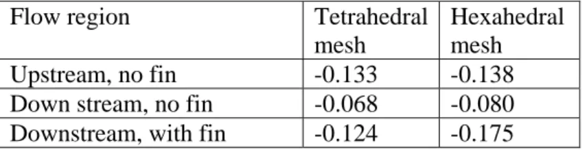
Through plane velocity components

Table 16 shows a summary of the non-dimensional errors in the through plane velocity components for each of the locations around the tug. In this table, the non-dimensional parameter Erroru was calculated from Tables 10 to 15 by non-dimensionalizing the values of ErrorVx with the free stream flow speed.

Flow region Tetrahedral mesh

Hexahedral mesh Upstream, no fin -0.133 -0.138 Down stream, no fin -0.068 -0.080 Downstream, with fin -0.124 -0.175

Table 16, Non-dimensional values of Erroru

From these values it can be seen that the value of Erroru is consistently negative. This means that the flow component from the CFD predictions was consistently higher than the observed values in the experiments. The difference was consistent with the values of the wake from the seeding rake used for these experiments (Molyneux, 2006c), which was seen to be between 10 and 12 percent of the free stream flow. It was likely that the wake from the seeding rake was reducing the flow speed, relative to the case when the rake was not present. It was also shown that the rake had negligible effect on the in-plane flow measurements, so comparison between the CFD simulations and the PIV

experiments should be focussed on the in-plane flow patterns.

In-plane velocity components

Three numerical values were picked to compare the PIV experiments with the tetrahedral and hexahedral meshes. These were the mean value and standard deviation of Error2D and the fraction of the data where the error between the CFD predictions and the experiments (for the in-plane flow components) were within 10% of the free stream speed. The values were non-dimensionalized based on the free stream speed of 0.5 m/s. The results are given in Tables 17 to 19.

These tables show that there was very little effect of the mesh type on the flow patterns, when compared to the observed flow patterns from the PIV experiments. The hexahedral mesh had a small advantage on the upstream side of the tug model, but on the

downstream side, the tetrahedral mesh had a slight advantage.

In general, the best predictions were for the upstream side of the tug and the worst predictions were for the downstream side of the tug, with the fin.

(41)

Hexahedral mesh Upstream, no fin 0.083 0.076 Down stream, no fin 0.074 0.078 Downstream, with fin 0.097 0.101

Table 17, Non-dimensional mean, Error2D

Hexahedral mesh Upstream, no fin 0.117 0.107 Down stream, no fin 0.049 0.055 Downstream, with fin 0.064 0.074 Table 18, Non-dimensional standard deviation, Error2D

Hexahedral mesh Upstream, no fin 0.827 0.840 Down stream, no fin 0.820 0.785 Downstream, with fin 0.623 0.598 Table 19, Fraction of data set where Error2D was within

10% of free stream speed

For the flow on the upstream side of the hull (Figures 27 and 29), both meshes gave similar errors, with the worst predictions of flow vectors close to the hull and the accuracy of the predictions improving as the distance from the hull increased. PIV measurements close to the hull will likely be the most difficult to obtain accurately, because the hull, even when painted black, reflects the light and a bright band is seen where the laser beam cuts the hull. Even though the analysis software includes a filter to reduce this effect, the experiment results obtained in this region may be subject to error. On the downstream side of the hull without the fin, (Figures 31 and 33) the highest errors were seen on the underside of the hull, just before the corner of the bilge, and on the top of the vortex caused by the flow separation at the bilge. In the region under the hull, the CFD did not predict the speed of the flow, especially for the tetrahedral mesh. In this case the predicted flow was almost stationary, whereas the PIV measurements showed it was

(42)

the region where the strongest flow velocities occurred. These high velocities were the result of the vortex caused by the flow separation off the corner of the bilge. Again the hexahedral gave smaller errors in this region but it the difference was not significant relative to the tetrahedral mesh.

When the fin was present (Figures 35 and 37) and the very large vortex was generated, the worst comparison between the experiment data and the CFD predictions occurred close to the hull on the downstream side between the bottom of the hull and the waterline, and under the hull. Both meshes showed relatively small errors in the flow around the vortex, but the hexahedral mesh gave relatively poor prediction of the flow patterns close to the waterline, compared to the tetrahedral mesh.

Based on the numerical analysis, both meshes gave acceptable predictions of the flow patterns around the hull of an escort tug with a yaw angle of 45 degrees, and neither approach had a significant advantage in any of the conditions investigated.

The non-dimensional values for the errors between the PIV experiments and the CFD predictions for the escort tug at 45 degrees yaw are compared to the Series 60 model at 35 degrees yaw (Molyneux 2006a) in Table 20 for the tetrahedral mesh and Table 21 for the hexahedral mesh. These tables show that the accuracy of the CFD predictions for the escort tug was better than for the Series 60 model, and the CFD predictions showed less variation with the type of the mesh.

Parameter Series 60, CB=0.6

Yaw angle 35 degrees,

Midship section

Escort tug, no fin Yaw angle 45 degrees,

Midship section

Escort tug, with fin Yaw angle 45 degrees, Midship section Errorv 0.091 0.024 -.010 Errorw 0.013 0.010 0.040 Error2D 0.241 0.074 0.097

Table 20, Comparison between Series 60 and escort tug, tetrahedral mesh

Parameter Series 60, CB=0.6

Yaw angle 35 degrees,

Midship section

Escort tug, no fin Yaw angle 45 degrees,

Midship section

Escort tug, with fin Yaw angle 45 degrees, Midship section Errorv 0.053 0.027 0.014 Errorw 0.049 0.003 0.041 Error2D 0.164 0.078 0.101

(43)

These differences may be due to the significant differences in the hull shapes between the escort tug and the Series 60 hull. The escort tug was proportionally much wider (L/B=2.69) and shallower (B/T=3.74) compared to the Series 60 hull with L/B=7.5 and B/T=2.5. The flow on the downstream side of the escort tug (between the waterline and the keel) was proportionally faster than the flow on the downstream side of the Series 60 hull, while the flow over the bottom was approximately the same. As a result, there was less of a shear force gradient on the tug and so when the vortex forms it will not be as strong as the vortex on the Series 60.

RECOMMENDATIONS FOR FURTHER STUDY

There are some improvements that could be made to the CFD mesh that might improve the level of prediction of the forces and flow patterns. The first major refinement would be to include the free surface waves generated by the hull. This was ignored from the current meshes, on the basis that the effect of the free surface on the forces measured in the model experiments was seen to be small. The free surface of the water will distort and may affect the flow patterns close to the surface. This effect may become more noticeable as yaw angles and flow speeds increase.

Another refinement would be to make the mesh elements smaller in key areas of the flow. The most likely areas for refinement are where vortices are generated in the flow. The most noticeable vortices observed in the PIV experiments were around the downstream bilge for the hull without the fin, and the large vortex generated by the fin when it was fitted. The refined mesh could be compared with the single measurement window PIV data, instead of the coarser data spacing that was used for the complete data set. The data from the single measurement windows is available on very fine grid points, but a

complete grid with cells at a similar spacing would be exceedingly large and require a very long time to come to a solution.

CONCLUSIONS

A commercial Computational Fluid Dynamics (CFD) code was used to predict the forces generated by an escort tug hull, and the same hull fitted with a low aspect ratio fin, over the typical operating range of yaw angles, from 10 to 60 degrees. Two types of mesh were used. One type was a tetrahedral mesh, consisting of elements with four, three sided faces. The other type was a hexahedral mesh, consisting of elements made of six four sided faces. The most accurate force predictions were obtained using the mesh made entirely of hexahedral elements. This mesh gave force predictions that on average were within 5-6 % of measured values for the same flow conditions, and never exceeded 10%. The number of elements for the hexahedral mesh was less than one half of the number in

(44)

comparison of the results indicated that the hexahedral mesh gave slightly better predictions of the flow patterns, especially for the flow conditions across the bottom of the hull. A numerical analysis comparing the two meshes over the complete measurement region indicated that the differences were very localized and numerically very small. When the data for forces and flow patterns were combined, the best approach for creating a CFD simulation of an escort tug operating at a large yaw angle was to use a hexahedral mesh. Earlier studies on the Series 60 (Molyneux 2006a) indicated that neither meshing approach had a significant advantage, but this conclusion was based principally on flow data and only included force measurements at 10 degrees of yaw. The different shape of the hull for the escort tug may have an effect on the accuracy of the predictions for different meshes, since this hull was wide and shallow with a high degree of curvature, whereas the Series 60 was relatively narrow with very sharp waterlines in the bow and stern.

ACKNOWLEDGEMENTS

I would like to thank Mr. Robert Allan, President of Robert Allan Ltd., Vancouver, British Columbia, for permission to use the model of the escort tug in the PIV

experiments and for the use of the experimental data on the force components to compare with the CFD simulations. His enthusiasm for the subject of tug design and his

encouragement for me to carry out this work is also very much appreciated.

REFERENCES

Allan, R., Bartells, J-E., and Molyneux, W. D. ‘The Development of a New Generation of High Performance Escort Tugs’, Proceedings, International Towage and Salvage Conference, Jersey, May 2000.

Allan R. G. & Molyneux, W. D. 2004 ‘Escort Tug Design Alternatives and a Comparison of Their Hydrodynamic Performance’, Paper A11, Maritime Technology Conference and Expo, S.N.A.M.E. Washington, D. C. September 30th to October 1st.

Fluent Inc. 2005 ‘Fluent 6.2 User’s Guide’ available on-line, July 2005.

http://www.fluentusers.com/fluent/doc/ori/html/ug/main_pre.htm

Fluent Inc. 2005 ‘Gambit 2.2 User’s Guide’, available on-line, June 2005

http://www.fluentusers.com/gambit/doc/doc_f.htm

Hutchison, B., Gray, D. and Jagannathan S., 1993 ‘New Insights into Voith Schneider Tractor Tug Capability’, Marine Technology, Vol. 30, No. 4, pp. 233-242.

(45)

Molyneux, W. D. 2003 ‘A Comparison of Hydrodynamic Forces Generated by Three Different Escort Tug Configurations’, NRC-IOT, TR-2003-27, LIMITED

DISTRIBUTION.

Molyneux, W. D. 2006a) ‘Evaluation of CFD Meshing Strategies for a Hull with a Yaw Angle, Based on Series 60 CB=0.6 Hull Form’, NRC-IOT, TR-2006-11

Molyneux, W. D. 2006b) ‘Particle Image Velocimetry Measurements of Flow Around an Escort Tug Model with a Yaw Angle of 45 Degrees’, NRC-IOT, TR-2006-18

Molyneux, W. D. 2006c) ‘Description of the Steroescopic Particle Image Velocimetry System Used by Memorial University of Newfoundland’, NRC-IOT, TR-2006-12