Beyond text analysis : image-based evaluation of health-related text readability using style features

Beyond Text Analysis: Image-Based Evaluation of

Health-Related Text Readability Using Style Features

by

Freddy Nole Bafuka

S.B., Computer Science & Electrical Engineering, M.I.T., 2006

Research Fellow, Decision Systems Group (DSG), Harvard Medical School

Submitted to the Department of Electrical Engineering and Computer Science

in Partial Fulfillment of the Requirements for the Degree of

Master of Engineering in Electrical Engineering and Computer Science

at the Massachusetts Institute of Technology MASSACHUSI

'urUN, OF TEC

May

2009

Copyright 2009 Freddy Nole Bafuka. All rights reserved.

JUL

The author hereby grants to M.I.T. permission to reproduce and

LIB

to distribute publicly paper and electronic copies of this thesis document in whole and in part in

any medium now known or hereafter created.

Author

Dep rtme t of Electrical Engineering and ComputeLr o..

/ May 27, 2009

Certified by

_{_}

William J Long Principal Research Associate, CoMputer Science & Art. Int. Lab, MIT Thesis Supervisor Certified by

Dorothy Curtis

Research Scientist, qomputer ience & Art. ±nt. Lab, M; DSG Affiliate

...

/ /

Arthur C. Smith Professor of Electrical Engineering Chairman, Department Committee on Graduate Theses

HIVES

ETTS INSTITUTE

HNOLOGY

0

2009

Using Style Jor Evaluation ofReadability of Health Documents-Thesis by Freddy N Bafiuka

Beyond Text Analysis: Image-Based Evaluation of

Health-Related Text Readability Using Style Features

by

Freddy N. Bafuka

Submitted to the

Department of Electrical Engineering and Computer Science May 28, 2009

In Partial Fulfillment of the Requirements for the Degree of Master of Engineering in Electrical Engineering and Computer Science

Abstract

Many studies have shown that the readability of health documents presented to

consumers does not match their reading levels. An accurate assessment of the

readability of health-related texts is an important step in providing material that

match readers' literacy. Current readability measurements depend heavily on text

analysis (NLP), but neglect style (text layout). In this study, we show that style

properties are important predictors of documents' readability. In particular, we build

an automated computer program that uses documents' style to predict their

readability score. The style features are extracted by analyzing only one page of the

document as an image. The scores produced by our system were tested against

scores given by human experts. Our tool shows stronger correlation to experts'

scores than the Flesch-Kincaid readability grading method. We provide an end-user

program, VisualGrader, which provides a Graphical User Interface to the scoring

model.

Thesis Supervisors:

William J. Long,

Title: Principal Research Associate, Computer Science & Art. Int. Lab, MIT Dorothy Curtis

Table of Contents

1. Introduction and Motivation

4

2. Background

5

3. Feature Extraction

12

4. Machine Learning Models Used

22

5.

Results

30

6. Discussion

61

7. Real-World Usage

65

8. Conclusion

68

9. Acknowledgments

69

10. References

70

Using Style Jbr Evaluation of Readability of Health Documents-Thesis by Freddy N Bafuka

1. Introduction and Motivation

Readability is defined as the ease with which a document can be read[1]. Many studies have shown that the readability of the health information provided to consumers does not match their reading levels[2]. Even though healthcare providers and writers have tried to make more readable materials, most patient-oriented web sites, pamphlets, drug-labels, and discharge instructions still require a tenth grade reading level or higher[3]. More than half of consumer-oriented web pages present college-level material[3]. A study by Doak et al found that patients, who may be more stressed, read on average five grades lower than the last year completed in school[4]. Misunderstandings of health information have been linked to higher risk of consumers making unwise health decisions, which in turn leads to poorer health and higher health care costs[5].

To provide more readable health texts, The Decision Support Group under Qing Zeng-Treitler at Brigham and Women's Hospital will develop a computer program to translate texts to a readability level

appropriate to several consumer reading levels. This program will be based on statistical natural language processing techniques. Providing health texts of appropriate readability to consumers should help improve comprehension, self management and, potentially, clinical outcome[3]. We envision the following scenario:

Gary is a diabetes patient with poor metabolic control. Laura, a nurse educator, talks with Gary about exercise and weight control. During their conversation, Laura senses that Gary's literacy level is inadequate for use of the latest teaching materials on the importance of exercise, which are written for average (seventh to ninth grade) reading ability. With the help of a readability adjustment software tool, she quickly generates a simplified version for Gary to take home. Because Gary can understand the

materials, he is motivated to follow their advice and exercise, which in turn helps to control his illness and prevent complications.

In order to translate a text from a higher to a lower literacy level, we must be able to correctly assess its readability. Having an accurate evaluation of a document's readability level provides guidance as to which tools or algorithms will be most appropriate for its translation to a more easily readable target. The goal of this study was to develop and a evaluate a new approach for assessing the readability of health-related documents.

2. Background

2.1 Previous Works

Several well-known word processing software products such as Microsoft Word, WordPerfect, and Lotus, provide generalized readability evaluation tools, using text analysis methods. Some of the features used in text analysis are extracted using Natural Language Processing (NLP) tools. In this thesis, we use the terms NLP and text analysis interchangeably.

Among the most widely used methods based on text analysis are the Simple Measure of Gobbledygook (SMOG) formula[6] and the Flesch-Kincaid grading formula[7], and the Gunning Fox Index (GFI)[8]. These methods computes readability scores based on text unit length, and yield scores that can be interpreted as the number of years of education needed to easily read the document. The Flesch-Kincaid method converts Flesch Reading Ease scores[9] into a grade-level. The SMOG formula computes readability scores using the number of sentences and the number of polysyllabic words-that is, words with more than 3 syllables. The GFI method uses sentence length and the percentage of

polysyllabic words.

While these methods perform well for general use, several studies have shown they are often inadequate for health-related documents, as they fail to capture many important features unique to health documents[ 10],[ 11]. In addition, some of the measurements used by these methods become inappropriate for the evaluation of some health-related fields[12],[13]. In particular, they do not measure text cohesion, or sentence coherence, which studies have found to be an essential part of easily understanding the English language[ 14],[15]. A study by Rosemblat et al[ 10] suggests that the "ability to communicate the main point" and familiarity with terminology should be considered as additional properties in measuring health text readability. In addition, a study by Ownby[ 13] suggests that vocabulary complexity, sentence

complexity and use of passive voice are the appropriate measures of text readability. Zeng-Treitler et

al[ 11] pointed out that electronic health records (EHRs), consumer health materials, and scientific journal

articles exhibit many syntactic and semantic properties that are unaccounted for by existing readability measurements. These are examples of text properties not measured by formulas such as Flesch-Kincaid,

SMOG and GFI. Hence, the need for specialized evaluation tools for health-related documents.

Several such specialized systems have been developed to evaluate the readability of health documents, using a Natural Language Processing approach. These systems are based on features such as

Using Style for Evaluation of Readability of Health Documents-Thesis by Freddy N Bafuka

frequency of certain parts of speech, sentence lengths, parse tree structures, text cohesion and so forth. Kim et al[16], for instance, developed a new readability measurement for health-related text, based on the differences in semantic and syntactic features, in addition to the text unit length already used by the general methods mentioned earlier. Zeng-Treitler et al[ 17], developed a new measurement of consumer familiarity with health terminology, which can be used as an additional predictor in assessing the

readability of health-related documents. These new types of measurements are providing better

assessment of health-related documents, where generalized methods might not be optimal. For instance, a common feature used by the generalized methods mentioned earlier, is the number of polysyllabic terms. A word with more than three syllables is considered a difficult word, and thereby increases the difficulty of the text that contains it, whereas words with fewer syllables are considered easier[ 18]. While this might be the case for general texts (in the English language), it is not the case when it comes to some health-related documents. Many words with same number of syllables can have varying levels of difficulty[ 17]. The word "diabetes", for instance, has 4 syllables but is generally a term with which a healthcare

consumer would be familiar. The words "aspirin", "Anbesol" and "aplisol" have same of syllable but varying difficulty level[ 17].

2.2 A New Approach: Style-based Features

While many text evaluation systems have used the Natural Language Processing approach, the effect of the layout of the text on readability has been very little-explored. In this study we show that a strong relation exists between certain textual layout features of a document and its readability level. We extract these features using an image-based approach. Rather than explore what the text says and how it says it, we rather consider how the text looks. Throughout this document we use term style to refer to text layout, and use both terms interchangeably.

2.3 Advantages of Image-Based over NLP-Based Evaluation of Text

Readability

This image-based evaluation, which converts the text into an image, presents several advantages over the traditional NLP approach.

Many of the features used in Natural Language Processing techniques for evaluation of text difficulty, fail when applied to health documents[ 10]. As mentioned above, the number of syllables per word may not always be an optimal indicator of the difficulty level of health-related text.

Secondly, health documents come in a variety formats: printed journals, pamphlets, medical records, web-pages, etc. An NLP-based system depends heavily and entirely on accessing the actual text.

Such a system would have to be able to parse HTML code, for instance, to extract the text of a web-page. It would also have to be able to receive a PDF as input and have the appropriate tools to parse that type of file as well. This need for flexibility in type of input adds a great overhead for an NLP-based system intended for general use. A commonly-encountered challenge with healthcare-related NLP tools, is that they are usually difficult to adapt, generalize and reuse[ 19]. Very few NLP-based systems developed by one healthcare institution have successfully been adapted for use by an unrelated institution[ 19]. One reason is that medical NLP tools are often overly customized to domain or institution-specific document formats and other text characteristics[ 19].

Moreover, some medical documents are not available electronically, but only in printed form. Some medical records, or hand-written notes by doctors and nurses are a common examples. An NLP-based system would not be able to process such document formats; the document's text would have to be extracted first. In an image-based system, however, the document can simply be scanned and the system can work with its image.

Lastly, the features used in NLP-based systems are not consistent across all natural languages. For instance, some languages have, on average, more syllables per word. An NLP-based system that uses such features would have to be retrained in each specific language in order to perform accurately. While natural languages differ widely in content, and features such as length of words, sentences, they are by and large similar in text style-a journal publication will almost always be formatted in columns, for instance; a title will often be in bold and bigger than the rest of of the text, etc. Therefore, it is unlikely that a system based on style will need retraining for use in another language. This language-independent aspect of the style-based system is a great asset in the health field, where patients come from various language and cultural backgrounds.

2.4 Previous Work on Text Evaluation Using Text Layout Features

While many studies have acknowledged the importance of text layout in assessing the readability of health documents, very little exploration of it has been done[ 17]. Two previous studies, Mosenthal and Kirsch [20], and Doak and Root [21], have explored text layout as part of a readability scoring scheme. Mosenthal and Kirsch developed the PMOSE/IKIRSCH method for measuring the readability of graphs, tables and illustrations, in turn giving a measure of the readability of a document. Doak and Root

Using Style Jbr Evaluation of Readability of Health Documents-Thesis by Freddy N Bafuka

layout and document design. However, these two systems are complex and not computerized. In this study we provide a fully automated, artificially intelligent approach to extracting various style features, evaluating them and constructing a regression model to map documents' style features to their readability level. As far as we know, there is no other computer tool of the kind we developed and present here.

2.5

Components of this Thesis

The general goal of the thesis is to assess the readability of health texts, using only the style of the document. More specifically, we would like to perform two tasks:

(i) Build a computerized model, which, given an arbitrary health-related document as input, will output a readability score for that document, using its style properties. We would like the score

given by the model to be as close as possible to the score that a human expert in readability would give to the same document. Throughout the rest of this thesis, we will refer to this task as the score prediction problem, or, the regression problem. We also use the terms score and grade

interchangeably, to refer to the numerical measure of a document's readability. We use the terms gold standard and target, to refer to the score given to a document by a human experts.

(ii) Build a computerized model, which, given an arbitrarily health-related document as input, will classify it as either easy-to-read or hard-to-read, using its style properties. We would like the classification decision of this model, to agree as often as possible with the decision of a human reader on the same documents. Throughout the rest of this thesis, we will refer to this task as the classification problem. We also use the term target or ground-truth, to refer to the class ("easy" or

"hard") given to a document by a human.

In order to rightly relate documents' style to readability score, or the easy- or hard-to-read classes, we will need three main components:

(i) A numerical representation of stylistic properties of documents. Chapter 3 details which properties (features) we chose and how we quantize them. We refer to this part of the project as the feature extraction step. Because we approach each document as an image, and use image processing techniques to extract the style features, we also refer to this part of the project as the

image processing step. We will often use the term feature to refer to an actual property (right margin, for instance,) and feature value, to refer to the actual measurement of that property for a specific document (e.g., "Document 1 has a margin of 0.1"). We also refer to the features as variables or predictors and use both terms interchangeably.

(ii) A machine learning model, which provides a mathematical relationship between the feature values of documents and their score or class. A machine learning model is built using a set of examples. In this project, an example is a document whose feature values and human-experts-given score or class are used as part of building the machine learning model with the optimal parameters that define the relation between document features and scores or class. We refer to this building process as the training of the model. We refer to the set of documents used in training as the training set. We evaluate the performance of a model by comparing its output

(score or class) for new documents (not used in the training set), to the score or class given by the human observers, for the same documents. We refer to this group of new documents used for the purpose of evaluating a model's performance as the testing set (or simply test set). Chapter 4 describes the various machine learning models we chose to use, and the processes by which we evaluate their performance. Chapter 5 reports and analyzes the results.

(iii) A set of documents from which we can create training and testing sets. More specifically, we needed three data sets: (1) a set of documents with scores given by human expert reviewers, to be used for the score prediction task; (2) a set of easy-to-read documents and (3) a set of hard-to-read documents. We consider the last two sets as one data set for the classification task.

Throughout this thesis we use the term data or dataset, to refer to documents, and in particular, the set of feature values extracted from them. We provide more information about the data sets in this section.

2.5.1. Feature Extraction and Image Processing

This project can be thought of has having a image processing step, which provides input to the machine learning step. The feature extraction part of this project uses some common image processing techniques. In particular, many of the features are extracted by detecting boundaries between text and background (or whitespace) regions. This process of breaking an image into meaningful regions for further analysis, using pixel similarities, is referred to as image segmentation[22]. Shi and Malik[23] presented a mathematical representation of image segmentation, as the segmentation of a connected graph with pixels acting as nodes connected to neighboring pixels by weighted edges. The segmentation task, then consists of minimizing the weights between pixels belonging to different objects and maximizing them for pixels belonging to the same object. That is also the basic concept we use to differentiate between text and background areas. Essentially, we attempt to extract some information on the presence of text on a page's image, by carefully canvasing through the page, and detecting regions with sharp changes in color intensity. The resulting feature values are then fed into the building of a machine

Using Style for Evaluation of Readability of Health Documents-Thesis by Freddy N Bajika

learning model, which makes a decision about the type document (easy vs. hard, or score). This technique is also similar to the one used in some object recognition methods, such as in the well-known face-detection system developed by Viola and Jones[24]. Viola and Jones searches a gray-scale image for rectangular regions of sharp changes in color intensity. These features are then used by a machine

learning model to recognize color-intensity changes that correspond to the set of boundaries need to form a human face. The Viola and Jones method however, uses human subjects to label hundreds of images of faces to form a training set. In this project, the feature extracted is fully automated.

Image segmentation is also used in Optical Character Recognition (OCR), to detect text in an image. OCR is very heavily used in the processing and routing of mail[25]. OCR systems also depend canvasing an image to find the text boundary, and the resulting features are used by a machine learning model to detect if a character is present and which character it is.

In the medical field, image segmentation is used widely in medical imaging for diagnosis, measuring tissue volumes, computer-guided surgeries and location of pathologies[26].

2.5.2. Expert-Rated Data Set

To provide a reliable set of documents for this and other health-related readability projects, the Decision Support Group under Qing Zeng-Treitler at Brigham and Women's Hospital carefully compiled

a corpus (dataset) of 324 health-related documents[27]. To obtain a diverse sample, 6 different types of documents were collected: consumer education materials, news stories, clinical trial records, clinical reports, scientific journal articles and consumer education material targeted at kids. Table 2.1 shows the

number of documents taken from each type.

Document Type Count

Consumer education material 142

News report 34

Clinical trial record 39

Scientific journal article 38

Physicians' Notes 38

Consumer education material targeted at kids 33 Table 2.1: Sample size of each document type used to form the 324-document data set with human expert score .

of Diabetes and Digestive and Kidney Diseases, and Mayo Clinic. The News report documents were taken from The New York Times, CNN, BBC, and TIME. The clinical trial documents were obtained from ClinicalTrials.gov. Scientific journal articles originated from the DiabetesCare, Annals of Internal Medicine, Circulation-Journal of the American Heart Association, Journal of Clinical Endocrinology and Metabolism and the British Medical Journal. Physicians' notes were obtained from the Brigham and Women's Hospital internal records. Lastly, the consumer education material for kids came from the American Diabetes Association.

With data collected, a panel of 5 health literacy and clinical experts and a patient representative were assembled to assess the readability of the 324 documents. Each expert was asked to grade the documents using a 1-7 scale. Each expert carefully reviewed and graded the documents independently. Many documents were graded by more than one experts. In those cases, we used the average of scores as the final gold standard for the document.

2.5.3 Easy and Hard-to-Read Data Set

The data of easy- and hard-to-read documents used in the project is a subset of the one used by Kim et al[ 16]. The easy data set consisted of 195 self-labeled easy-to-read health materials from various web information resources including MedlinePlus and the Food and Drug Administration consumer information pages. They covered various topics on disease, wellness, and health policy. The hard dataset consisted of 172 scientific biomedical journal and medical textbook articles on several topics, including various diseases, wellness, biochemistry, and policy issues.

Using Style for Evaluation of Readability of Health Documents-Thesis by Freddy N Bafuka

3. Features Extraction Method

The first implementation work was done on MATLAB R2007a, on a Dell Pentium Dual-Core, Windows Vista machine. In an effort to make the system more freely accessible, a Java implementation was also done, on the same machine. We present the details of both implementations later in this document. There are slight variations in the two implementations. We mention those when necessary, throughout the description of the method. Given that the Java implementation is the latest, contains more features, we consider it the main implementation of this paper, and the one that we expect others to use

3.1 Conversion to Image Format

There were 324 expert-rated documents used, with readability scores ranging from 1 (easiest to read) to 7 (hardest to read). Additionally, there was a set of 195 documents simply considered "easy to read", compared to another set of 172 documents considered "hard to read".

Each document was converted, from its original format, to a set of images, with one image for each page. However, we used style features from just one page-the "first page" of the document. Cover pages, and table-of-content pages, and title pages were ignored. Hence we refer to the "first page" of the

document as the page in which the actual content of the document begins. The size of the images obtained from the documents differed, depending on the original format and size of the document. All images were converted to gray scale, with possible pixel values of 0-255.

Feature Extraction and Evaluation Pipeline

For each document, the following steps are followed to extract the features. * Document is converted from its original format to an image format. * Each page is converted to one image.

* The image is converted to gray-scale.

* Each resulting image is preprocessed and a new image is returned.

* The preprocessed image is sent as input to the DocFeatureExtractor module, which returns a numerical value for each feature, for that image.

Features Extracted

extracted were:

- Average white space (WSR) - Number of columns (CLC)

- Number of lines per column (LNC) - Left margin size (LMS)

- Right margin size (RMS) - Average gray-scale value (AGS) - Top margin size (TMS)

- Bottom margin size (BMS)

- Interline Space to Line Size Ratio (LSR)

- Interline Space Ratio (ISR)

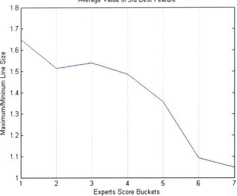
- Maximum to Minimum Line Size Ratio (MMR) - Number of Colors (CLRC)

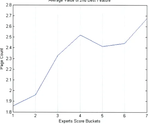
- Number of Page (PGC)

The extraction of these 13 features is detailed in the following subsections. Not all features where used in testing the MATLAB implementation. In particular, the interline space ratio (ISR), the number colors and the number of pages, were not used.

A few assumptions are made throughout the feature extraction stage. One is that the background color is lighter than the letters' color. The background value is determined taking the average pixel value of the 4 leftmost columns of pixels. Another assumption is that all pages have a left margin with a width

of at least 4 pixels.

3.1.1 Number of Columns

The number of columns in a page is determined by scanning the image of the page from left to right, examining a vertical strip that extends from the top to the bottom of the image, and has a small

width (equal to 1% of the total width of the image). The average value of the pixels within this vertical strip determines whether the strip within margin region or within column region. If the average value is less than value of the background minus 1, the vertical strip is considered within column region, otherwise, it is within margin region. The number of transitions from margin to column and vice versa indicates the number of columns in the document. Note that in the Java implementation the value of the

Using Style for Evaluation of Readability of Health Documents-Thesis by Freddy N Bafuka

background is always 255, on a traditional 0-255 gray-scale (please refer to the preprocessing steps described later in this chapter). This step was not taken in the MATLAB implementation.

3.1.2 Number of Lines Per Column

The lines within a column are detected with the same algorithm used for column detection. The image is rotated 90 degrees counter-clockwise, and each line is detected as if it were a column. However, the value of some of the input parameters to the algorithm are modified to detect lines. The width of the vertical strip is exactly equal to 1 pixel, given that spaces between lines are much smaller than spaces between columns. The 1-pixel width was determined by trial and error.

3.1.3 Average White Space

The average white space was computed by measuring the width of the space unoccupied by letters at the beginning and at the end of each line in a column of text. The sum of this width for all lines, divided by the sum of the total width of all lines, gives the average white space ratio. To determine the space unoccupied by letters in a line, the line is scanned from left to right, until non-background color is detected. A similar technique is used by scanning from right to left, to find the width of white space at the end of a line.

Meal Planning

Some people with diabetes use carbohydrate counting to balance their food and

insulin.

Carbohydrates,

or "carbs," are what our

bodies

use for fuel. The more

carbs

you eat, the higher

your blood

glucose goes. And the higher your blood

glucose, the more insulin you need to move the sugar

into

your cells

Figure 3.1. An illustration of the whitespace feature, which captures how much of the

width of each line of text is unoccupied on both the right and left sides. In this example, the gray lines show the whitespace on the right side.

3.1.4 Margins and Gray-Scale Value

The left margin is determined by the width (number of pixels) of the space between the left edge of the image and the start of the leftmost column. The resulting value is divided by the total width of the image, and gives the margin value used as feature. The right margin is computed similarly, using the width of the space between the end of the right-most column and the right edge of the image.

Likewise, the top margin is determined by the length of the space between the top of the first line of text and the upper edge of the image, after preprocessing. Since the various columns of text might not start at the same line-that is one might be shifted down vertically, as is sometimes the case with first column, especially-the "first" line of text refers here to the first line of the column with the highest top edge. As lines within the columns are detected, the value of the highest line is updated as necessary. Similarly, the bottom margin is determined by length of the space between the bottom edge of the lowest line and the bottom edge of the image, after preprocessing. We also account for the fact that one column be "shorter" or end higher than others-as is often the case with the last column of text. Therefore, the

value of the lowest line is updated as the columns are scanned through during line detected. The line with the highest Y-value (lowest line) is retained for bottom-margin computation.

The average gray-scale value of the page is a simple average of the value of all pixels in the image. It gives an indication of how "dense" the document is.

Using Style for Evaluation of Readability of Health Documents-Thesis by Freddy N Bafuka

Figure 3.2a. The widths of the orange rectangles are left and right margins. The heights

of the light green rectangles are the top and bottom margins. The blue rectangle is the

inter-column space, which we use to detect columns.

rMWO. S RICHTS

7 w fnSwmeA ymnwAs adVO mRm

NowPeSumr-Y honimlno by takave In. l

daC*i art "ow n N4.ma (rq in to~s m At :kthrw L-! Vnmared 111 3 ary 11n trl Ms cw*d. a1 army 4 drts t. .tnC :Nxy a t 1.W 4,.n*m . trAwri. mrd *rwng ,ai4ne .an** ra.3-11 5. 3: r.waj N

twear

Sau

w

,%V f * *.1S X1**744 1 1 -OM n13* I U*V

hb Fnwo Me11 AL14 *= Tim 41.EIN

=*1da1 had .4 11 3 md a.:abase= wm*4 aMhr in U~. 34.aas ,y

1 4

u 111113311 111.1 33*141 *r

h and #1a 3 *1 ,rtmdn Amni nr m ti*m7

in " bemd hmsh 4err

wkw--Al I rte dro any d6imsura ahns ch dm P aghpan 5irln a maiLnUa~resI

Anta

PV# Ashon, xwsfawm iMq ad WA pn d A-, CA4

oamm 3.meamn o1 am, sm Wm =4 d*! ,m4 .. d4 1

stimma (.KE 1h 0 L-M owparm ag. n40 dA*' twh

as"W smew had rt ild w any tho kt mmmr

f 1:%%4 and .43ma .

remedmv"n* sh. 6imvaA --hat dU W. daumms h4

11h you and, a*.&AWwand armAd th W1 w

-mrn wa.y 1Asm Ir. me4= a .31mm a ha 4r,s

A4.mump A.11*m1 wa*411* adMh a1 .ahts.

AWN hp6 zatm

~

=a ad &AdwWWc of dch*f r*A m asMany

rhl-hAg wwn =L umsev Arsg t w m dt* hea da ta

dwar wr now mart a a as!an A U amhom n

AtL ANiTi PndalA AIANnn a So == s m4

bool W _na1

drg & panetakdmmr

~

yniaor :. ak Was = no A0%ktesan neam shnid ho

Pidrest trCid qW T? of = da mLaWr hyV 214t, rAM ,0 ar's may chu'm mdAd up us a644 ramps

w+Nm ohm uad thony nuso es uS om any 7aam whn masrmw m* rh-ta me:wd

hp* shO uppe Was imFm sa wwn & Vy " VW7 a aat&Oa W& AM MaWMmay wma pmred mw

*wk Ms wom Prefty admg Wh Atho de adewmk

OW WUN; YM341d * 2 OrPAC Wh O&W ft" s=

mimm rampa rh had Ama d e tb man wam tAh -mlinc Who si~yr WXA tarl Cis.-Ilamm- =Wat VmM washr wim dwy msand deah~ Iddt meb

am

,Am ski (0 mumm mudand Volk thar wMP 4

bwmn d&pn maL psnue and snay auda don

m ramoer# W sup ma thifa t En r d apng Mr =a

=a e.&w rampl s. swa

:' m~ z Lm pn~e unrn#

t?"mmi-And ascam rdmjb- fe Ldn weorr* a't m -h.waymwna nondr V*I'A

A ?RI VAITJ CEiZBRAI1L

'Arm :n tim* -im Z dwl e skn a mr ctew

wa n mwed wm. r"t r uiw fdmawgn a'i LhOA

-and yma - insem vAw wth t d= u a! 4vhn

11WORS f Wi Ad r, i n "rr*WWWAM~ 1.4Jsdn nf rW

uhzshms irm zwm Ywiam Marm chk:Wo wa

d11a a d1a 3m;Wamr1m flfid% Engenn and 4m

Pasher ::A % k # Wvatro wdme d d

m

wao "WA.va l.y r? Xin a*nd1 n r

r m. a my ivi : wL toum tim mm1r al

nar wy w:-r pa* wVl * a werY bfles i

:n m MWn, :w . FAqd 1 W=s anm u dmar

Aw (7ira:00=0" ni My -,amna bw ,ape V MFM im

%maal a,*M. JA.n1wd Ira nm IIR aMA n a

d~ap mrry kjlgnu a tIrm anolmen w WiEAVTI' fl3SPECIT 'VFo1W AS 1610A' MION C VM a;md an =n=m a rrrar and a b" ww inod a

dmeran d wanM .

: am d m1.1 to my thar h. n:*padAmd Irssm d

Wl; *111P B 3*31. *113! .131 4111 I, II .II.*h

mml nmnwkm and mham pma stAim w3 wave w au.rF3nay ow ni mm and 1te prwma w1 i Ararmed by d a -hs-Wh r waq mPldt whoAm

rwdiw mrJ ao sm nd w-b yjmem tham im

#gs a 3

WmI*w &Wmmmwvd wnam on tmam n

04r: * hr pumi a 1ng !MWMpd l atumatv.e1Ud

NArAng rwr I wush 2 wPL and : iam &,Am tm or

aibaitrm w hm vrmy I aA

H ALTH PERSCM VR N UMAN e.mHTS

Arl xwm M. 'flu m r0 , 1d b kmw g a

ummfmt h o d uwa nwI mSWandnd, aquft

Ma pva nmesu smmmmiri Wyms inma tm hmmsh

vmskon r awd nd ma ams fin dpMany V m"N rnimAl

Tin mantannawal -boa

Tm Featmar t twram VWompt a wa i to armo of our

aman, ho Ra*i me XapmJ deat mthrt eghts ad 06M hQussaMa rmanashmid MA sMWd MW 1j"

040m0ba=S 6W OdmaWWg hAftA ram Vadma MinW A iaso aman aNManis 2amrW~a# O Am mInanf

dM6 lawn dr Ar od homid

Or h eatl Alurmmani mhoen ddmm AmAwrven fit tiar mw af n M glea dnghi acq and

paradean at hmb raw Mm ww goemy amannd do

homfid am af radod a n wWA by many presr

mmwdysnr~r arpllbndrshrthanWa nan est

Ahm wus Ad th do wraid Was ek Atvwwe harmw

hme whm n w and hIan wh inv" me drtlrr.

Figure 3.2b. The original image of the page used in figure 3.2a. Note the footer was

ignored. The bottom margin is the height of the space between the bottom edge and the last line of actual text detected.

3.1.7 Interline Space Ratio

The purpose of this feature is to capture the sparsity of the of text. This feature captures how much the vertical space is occupied by lines of text, and who much is background. It is analogous to the "average white space" features, which computes horizontal white spaces. It is computed by adding up the heights of all lines of text within each column and dividing that value from the total height of the image. The resulting value, subtracted from 1, gives the interline space ratio.

Figure 3.3 shows the interline space.

ir~knrzn np~rl

Using Style for Evaluation of Readability of Health Documents-Thesis by Freddy N Bafuka

Figure 3.3a The interline spaces (heights of the gray

rectangles shown above. As can be seen the interline space

can vary greatly between different pairs of adjacent lines.

FINDINGS

Post

Mond&y, June 13, 2005; A09

Diabetes Treatment Helps Babies' Health

Women who develop diabetes during pregnancy give birth to healt aggressively treated, according to a large study that helps bolster t pregnant womn for diabetes.

In the study, Australian researchers followed 1,000 women diagno diabetes. During their third trimester, the women were separated i

Figure 3.3b. The original image used for illustration in

figure 3.3a.

3.1.8 Interline-to-Line Size Ratio

This feature further captures the sparsity of the page. It completes the previous feature in that it would capture the difference between a single-spaced and a double-spaced document. For instance, a page with two line of text using 60-point size font will yield the same value for the previous feature, for 12 lines using 10-point size font. The spacing between the lines might not have changed. This feature, therefore, finds a ratio between the average size of lines of text and the average size of interline space. Scientific papers for instance, when published in a journal, will tend to be single-spaced and denser. The line-to-whitespace ratio is computed by adding up all the line sizes and all the interline spaces (heights), and taking the ratio of the two numbers. In figure 3.4, we show the line sizes. The interline spaces are

FINDINGS

},

)interline

space

M .amy, Jmun 13. 2005: A09

Diabetes Treatment Helps Babies' Health

Women who develop diabetes durin pregnancy give birth to healt aggressively treated, according to a large study that helps bolster t pregnant women for diabetes.

In the study Australian researchers followed 1.000 women diasno diabetes. uring their thrd trmester the women were separated n

shown in figure 3.3a.

FINDINGS

}

Line

Size

Nvldv. , ue 13.2t' : A0.

Diabetes Treatment Helps Babies' Health

)

Women who develop diabetes during pregnancy give birth to healt aggressirely treated, according to a large study that helps bolster t pregnant women for diabetes. I Line Size

In the study, Australian researchers followed 1.000 women diagno diabetes. During their third trimester, the women were separated m

Figure 3.4. In red, 3 different line sizes are pointed out.

3.1.8 Maximum-to-Minimum Line Size Ratio

The maximum-to-minimum line size ratio tries to capture the variation in font size in a document. A value of 1 will mean that the same font size has been used throughout the page. A value of 6 will mean that the biggest line of text is 6 times larger than the smallest. Such a large ratio will probably indicate that several font sizes were used between the biggest and smallest one, which, in turn, indicates that the document is complex-the number fonts used give an indication to the number of subheadings used in the document.

3.1.9 Color Count

The number of colors in each document was extracted by search through each pixel of the page's image (before its conversion to gray-scale). Each color was assigned a unique number, by multiplying each of the color channel (red, green, blue) by 1, 103_{, and 106, respectively. From each pixel of the image,}

the color was extracted as a unique. That number was added to a set. Once colors had been extracted from all pixels and added to the set, the number of elements in the set indicated the number of colors in the image.

3.1.10 Number of Pages

This is the only feature that is a property of the whole document, and not of one page. The number of page per document was extracted by searching through the directory of images counting the number of images associated to the same document. Each image is interpreted as a page. Documents with more than 3 pages were given a page count of 3.

Using Style fbr Evaluation of Readability of Health Documents-Thesis by Freddy N Bafuka

3.2 Preprocessing Stages

Before the above features are actually extracted and evaluated from a page's image, a few preprocessing steps occur.

3.2.1 Pixel Value Extrapolation

To further create a clear demarcation between the text line areas and background, darker pixels are given a value of 0 on an 0-255 gray-scale, while lighter colors are extrapolated to 255. This

extrapolation eliminates unwanted side effect such as anti-aliasing, caused by graphic renderers.

3.2.2 Horizontal Slide Preprocessing

Even within the text regions of a document's page, a large amount of space is background. As a result, the average pixel value within text region can still be very close to background region. We therefore add a preprocessing step to increase the number of dark pixels within the text region. The step consists in "sliding" the image horizontally, on itself, which causes a thickening of the letters in the horizontal direction. The result is greater contrast between margin (just background) regions and text regions. See figure 3.5.

many health problems are linked to obesity. A person's body fat percentage gives a good indicator of whether they are obese. Hence body fat percentage is widely suggested as one

Figure 3.5a: Original image before horizontal slide.

MEW

hWl

h

ib

mr

n

ullo

d to obsia A

pm

bo

d

t

pMeatapl

-l£

a loo

dlae tor

whth thy

0

obl. MXm bodyt rct i ily

o llt

d

on

/

3.2.3 Non-Content Text Removal

Often, some documents come with text that should not be considered part of the document. For instance, when printing a web page, the web browser usually introduces a header or footer containing the URL of the web page being printed. Such a header would cause a misrepresentation of the top margin, for instance. Therefore, as an extra preprocessing step, we remove all text that are "too" close to the edges.

3.2.4 Differences between the Java and MATLAB Preprocessing

The Java implementation does not use the horizontal-slide processing, for usability reasons, as the implementation is very slow, where as the operation is fairly rapid in MATLAB. The pixel value

extrapolation was the best alternative to accentuate foreground vs. background differences. The MATLAB implementation, on the other hand, does not use pixel extrapolation, as the horizontal-slide provides adequate accentuation of the areas. Our results later showed that either method provided adequate ability to extract features correctly. We recommend that any implementation use at least one of those two preprocessing steps.

3.3 Extraction

The feature extraction was done on all documents without failure, although with some warnings from the ColumnDetector module. Two types of situations can cause the ColumnDetector to trigger a warning. First, there are cases in which the right boundary detected by the system happens to be such that a few lines in the column extend slightly beyond it. This normally happens just before the right margin of the document, when the text is left-justified, for instance. As the scanning progresses, the portions of lines extending beyond the column boundary can trigger a false column-start event. Usually, no end will be detected for such a false column, until the scanning reaches the right edge of the document. In these cases, the system infers that a "false end column" was started after the right boundary of the column, and ignores it. The Java implementation prints a warning on the standard error, stating "Warning: false end column. Ignoring..." Note that in this case, there is no failure, but rather a prevention of one. The second type of warning occurs when a column was started much earlier in the document--closer to the left edge-and yet no end to the column is detected till the scanning reaches the right edge of the document. In this case, the end of the page (right edge) is considered the end of the column. The Java implementation prints a warning on standard error, stating "Warning: column end was not found. Assuming end of page..." The MATLAB implementation throws a waming as well, but does not use different warning statement to distinguish between the two cases. Of the 324 page images used, less than 30 generated a warning, and virtually all were warnings of the first type.

Using Style for Evaluation of Readability of Health Documents-Thesis by Freddy N Bafuka

4. Machine Learning Algorithms Used

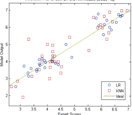
To predict the scores of expert-rated documents, we needed a regression algorithm, since the scores values are continuous-not discrete. We chose to train and test two different regression models:

(i) Linear Regression (ii) k-Nearest Neighbor

To classify between easy-to-read and hard-to-read documents, we needed a classification algorithm. We chose to train and test two classification models:

(i) SVM

(ii) Logistic Regression

From each document, one page was used to extract style features-except, of course, for the page count, a property of the entire document. The Java feature-extractor module extracts 13 features per document, while the MATLAB implementation extracts 10, as discussed earlier. For the purpose of this section, we will refer to m as the number of features extracted per document. For the Java

implementation, m = 13 and for the MATLAB counterpart, m = 10. We refer to the set of m feature values extracted from a particular document as the input from that document.

Let D be the vector of inputs D = ( DI, D2, ..., D,)'obtained from a particular data set. For the

expert-rated data set, n = 324. For the easy-to-read and hard-to-read data set, n = 195 + 172 = 367. Each input Di = ( da, di2, ... , dim) is a vector of feature values extracted from the i-th document in a given data set. Therefore, D can be thought of as a n-by-m matrix.

Let G be the grade given to the i-th document by the experts, in the expert-rated data set. G can therefore be thought of as a n-by- vector, with n=324. And let L, be the label (0 for easy, 1 for hard) given to the i-th document in the easy- and hard-to-read data set. L can therefore be considered an n-by-1 vector, with n = 367.

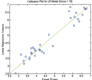
4.1 Regression Models for Prediction of Experts' Scores

In the prediction of the experts' scores, our goal is, ideally, to create a score function S such that S(D,) = Gi. In practice, however, we expect some level of error, which we define as: error(i) = Gi- S(Di)|.

4.1.1 Linear Regression

linear function of the variables. It often provides an adequate interpretation of the effect of the inputs on the output values[28]. In the next section, we consider an alternative model that does not make the assumption of a linear relationship between input and output.

Linear regression attempts to formulate S(Di) as follows:

S(D,)=0o+Z dij (4.1)

j=1

where the m+1 constant coefficients (also called parameters) ,fo, fl, ... , 8m are unknown. Taking all inputs, or observations into account, we can rewrite equation 4.1 as follows:

S(D)= + Y0D. .j (4.2)

j=1

where D: j represents thej-th column of D.

The constant coefficients make S a linear model. The essential part of training this linear regression model is finding the best set offlj parameters. There exists several criteria for determining the

"best" set of fj values. We chose to use the residual sum of squares (RSS), which is the most widely used measure for comparing such sets of parameters[29]. Given a vector of parameters fl = (fro, f , ... ,m), we define the residual sum of square as the sum of the square of the errors:

RSS()= (G - S(D))2 (4.3) i=1 RSS ( ()= (Gg-fo-# du j)2 (4.5) i=l j=1

We therefore define the best value for the vector of parameters fl as follows:

I = argmin RSS (g) (4.6)

We found the best set of parameter values by using MATLAB's glmfit function. The glmfit function takes two main inputs:

(i) An n-by-m matrix, representing n observations (in our case, document inputs), each having m predictor values (in our case, feature values). For this input, we provided a K-by-m matrix

constructed from K rows of the matrix D described above. We describe this further in the cross validation section later in the paper.

(ii) An n-by-1 vector, representing the target values. In our case, the targets are the experts' grades. For this input, we provide a K-by- vector constructed from K corresponding elements of G

Using Style for Evaluation of Readability of Health Documents-Thesis by Freddy N Bafuka vector described above. We give more details in the cross-validation section.

(iii) A specification for a distribution. We used a "normal" distribution, which causes gimfit to apply linear regression as formulated in equation 4.1. We used the default values for all other inputs to glmfit.

The g mfit function outputs a vector of m+1 elements, containing the values for flo,

fl,

Given a new document, D,, never seen before by the system, our model will predict its score by evaluating S(D,), using formula 4.1, with the parameter values obtained from glmfit.

4.1.2 k-Nearest Neighbor

The k-Nearest Neighbor algorithm is a memory-based system and does not require any search for best-fit parameters. Each input Di can be thought of as a point in a m-dimensional space. Given a new input D, never before seen by the system, we find the k closest points in distance to D, and compute its score by taking an average of its neighbors. We use Euclidean distance. Let K be the set of the k closet points to D,. We formulate S(D,) for k-nearest neighbor as follow:

S(D,)= -Y Gi (4.6)

ieK

Throughout this project, we used k= 3.

Despite its simplicity, k-nearest neighbor, it is known to perform well, and has been used successfully in many applications, include some image-processing related tasks[30],[31]. We use it as second alternative to linear regression, as it does not make any assumption about the linearity of the input-to-output effect.

4.1.3 Training and Testing Using Cross-Validation

For both the linear regression and k-nearest-neighbor models, we used a 5-fold cross-validation to run a training-testing cycle.

(i) Linear Regression

The 324 inputs in D were randomly placed into 5 folds (or partitions) of approximately equal size (4 of the 5 folds had 65 inputs, while one had 64). The first fold, FI, was used as test set, while the other 4 partitions were combined to form a training set. Given the inputs in the

training set, and their corresponding grades, we used the glmfit function to find the best set parameters for a linear regression model, as discussed in section 4.1.1 above. The resulting parameters were then used to apply the score function S to each of the inputs in F, according to equation 4.1. We then repeated the experiment (second cycle) using F2, the second fold, as the test

set and join the remaining 4 others to form the training set. We did the same for folds 3, 4 and 5, running 5 cycles total.

For each of those cycles, we recorded the average error. Let Ri be the set of inputs used for the training set when Fi is used as the testing set. And let Si be the score function with the beta values obtained by using R, as input to glmfit. We define the average error for a cycle i, avgErri as follows:

avgErr,=1 Gj-Si(Dj) (4.7)

avgE Fi D F

-We define the final average error for linear regression as follows:

5

avgErr 5= avgErri (4.8)

5 i=1

We repeated the whole experiment several times, randomly generating 5 new folds each time. We found that the results were relatively the same.

(ii) k-Nearest Neighbor

In a similar manner to the process described in part (i) above, the 324 inputs in D were randomly placed into 5 folds. The 5-KNN model was tested on each of the fold, while using the remaining 4 partitions as a training set. For KNN, a "training" set is simply the set used as the memory from which the k closest points to a test point are taken. There is no actual training stage comparable to the one for linear regression. More formally, in this experiment, if R, is the set of inputs used for the training set when Fi is used as the testing set, then we define S, as in equation 4.6, with the added constraint that K is strictly a subset of Ri . With Si thus defined, we evaluate each Si (Dj) for all Dj in F . We perform this routine for all 5 folds. We also compute and record the average error exactly as described in section (i) above (but with using Si as defined in this section).

Using Style or Evaluation of Readability of Health Documents-Thesis by Freddy N Bafuka

4.2 Classification Model for Recognition of Easy vs. Hard Documents

4.2.1 SVM

We use the Support Vector Machine (SVM) algorithm to build the first classification model. SVM treats the inputs as data points in an m-dimensional space. As mentioned earlier, m is the number of features (predictors) of each input. Given data points from two different classes, the SVM algorithm attempts to find a boundary line, plane or hyperplane (depending the value of m) that spatially separates the points of the two classes into two regions. The SVM method uses just a few points from each class, called support vectors, that lie at the boundary of the classes[32]. The assumption is that points at the boundary are the ones that are critical for defining a separating line. The line (or plane, or hyperplane) is chosen so as to maximize its distance from the support vectors on both regions.

Given a new, unseen data point, an SVM model will classify it based on which side of the boundary it lies on. Therefore, the output of our SVM model is binary: either a 0 (easy-to-read) or a 1 (hard-to-read). It is possible that a test point would fall on the separating hyperplane. In that case, the point's class is ambiguous, and it is not classified. Such a point is also not included in the classification accuracy measurements we describe later. It is also possible for a point to fall on the wrong side of the separating hyperplane-and in that case, it is considered missclassified.

We used MATLAB's implementation of the SVM algorithm, provided through the svmtrain function. The svmtrain function uses a linear kernel by default, which means that a simple dot product is used to determine the location of a test point with respect to the separating line, and the input is not transformed into another space (which is useful in some applications). The svmtrain function takes two arguments:

(i) An n-by-m matrix containing n observations, each having m predictors. In our case, we provided a subset of the matrix D of document inputs described earlier in this section.

(ii) An n-by-1 vector containing the ground truth values for the inputs given as the first argument above. For this argument, we provided the corresponding subset from the L vector of labels, described earlier.

The svmtra in function returns the bias and slope values for each dimension, for the separating hyperplane.

4.2.2 Logistic Regression

Given an input, the SVM model gives us only its class label as output. It would be useful to have a measure of confidence for the classification of a document. Logistic regression is a mathematical model that provides a real value as raw output. The output, which is always between 0 and 1, can be interpreted as the probability that a given input is of the positive class--"hard to read", in our case. The higher the value, the more likely the document is hard to read. The smaller the value, the more like it is to be easy to read. How high the value of the output must be in order for the input to be classified as hard-to-read is a question that we analyze, in a search for the appropriate cutoff threshold. Logistic regression is regarded as an efficient supervised learning algorithm for estimating the probability of an outcome or class variable. In spite of its simplicity, logistic regression has shown successful performance in a range of fields. It is widely used in a many fields because its results are easy to interpret[33].

Let Di be a document from the easy- and hard-to-read data set, as described earlier. We define a variable z as follow:

Z = B0+

8dil

B

where the for fo, i, ... , fl,,, are the unknown parameter values. The logistic regression model is described as follow:

+(z)= _(4.10)

l+e-'

The output from this function, 1(z), is what we define as the "raw output" of our logistic

regression model. From equation 4.10, we deduce that higher z values will produce an output closer to 1, while smaller z values will yield raw output closer to 0. Hence, the key part of building the appropriate linear regression model is to find the best set of parameters that will produce raw output close to 1 for the hard documents and close to 0 for the easy documents. We can also use the residual sum of squares to evaluate the best parameter values, as we did for linear regression earlier. Given a set R of documents labeled either 0 (easy) or 1 (hard to read) and a vector fl of parameters, we can define the RSS formally, for this case, as follows:

RSS( )= I (L-l(z))2

(4.11)

D ER

Using Style Jbr Evaluation of Readability of Health Documents-Thesis by Freddy N Bafuka formula 4.11 above).

We found the best parameters again by using MATLAB's solution implemented in the glmfit function. The arguments passed to glmfit in this case are similar to those described in section 4.1.1, except that the observations are taken from the easy- and hard-to-read data set, the target values are correspondingly taken from the L vector described earlier, and we use "binomial" for the distribution argument (so that glmfit computes the parameters based on equations 4.9-4.11)

4.2.3 Training and Testing Classification Algorithms

(i) SVM

We used a 3-fold cross validation scheme to train and test the SVM model. The 367 easy-and hard-to-read documents were reasy-andomly assigned to 3 folds of approximately equal sizes-2 of the folds having 122 distinct documents each, and one having 123. We performed the first iteration (or cycle) of training and testing by using the first fold, F1, as a test set. The remaining two folds were combined to form a training set, R1. R1 being therefore a 244- or 245-by-m matrix,

was used as the first argument to svmtrain, as discussed in section 4.2.1. The corresponding ground-truth labels, a vector of 244 (or 245) elements, was passed as the second argument to svmtrain.

The testing stage consisted of using the hyperplane obtained from svmtrain to classify the 122 (or 123) inputs in F. The number of misclassified inputs was noted. We define that number as the error for the iteration. We performed a second and third iteration in the same manner using fold F2, and F3, respectively, as the test set. For each iteration, we also noted its error. The total

error was obtained by adding the 3 error values obtained from the 3 iterations. We define the average error of the SVM model as the total error divided by the total number of inputs tested through all iterations, 367. We report the correct rate, which we define as 1 - average error.

(ii) Logistic Regression

To build a logistic regression model, we also use a 3-fold cross-validation scheme, as described in the previous subsection. The 367 data points were again randomly placed into 3 folds of approximately equal sizes. During each one of the 3 cross-validation iterations, one of the folds was used as a test set, while the other two were combined to form a training set. The training set was used as the first argument to glmfit (the observations,) as described in the previous section.

The corresponding labels, a 122- or 123-element vector, was used as the second argument-the vector of targets. We obtained the best set of parameters from th glmfit function's output. These parameters values were substituted into equation 4.9. We then obtained raw output values for the

inputs in the test set for the iteration, using equation 4.10. So, once all cross-validation iterations had been run, we had three logistic regression models, each with its set of optimal parameters, and a raw output value for each of the 367 inputs, corresponding their use as part of one the test set associated with their fold.

In order to test the performance of the logistic regression model, we needed a threshold to use as cutoff between the two classes. A document whose raw output value was above or equal to the threshold was considered of class 1 (hard to read). A raw value below the threshold classified the document as easy to read (class 0). The threshold could be any value in the [0 1] range. However, given the finite number of test inputs, only a finite number of threshold values would make a difference in performance. Hence, we considered potential thresholds only at the raw output values. That is, each raw output value was tested as a potential threshold. Therefore, we tested a total of 367 threshold values.

For each threshold value, we computed the true positive rate and the false positive rate. The true positive rate, also called the sensitivity, is the fraction of the positive test points that were correctly classified (as positive). In our case, the true positive rate is the number of hard

documents whose raw output values were equal to or above the threshold (i.e., correctly

classified) divided by the total number of hard documents in the test set. The false positive rate is the fraction of incorrectly classified negative samples. In this testing stage, the false positive rate is the number of easy documents whose raw output values were equal to or above the threshold (i.e, classified as hard) divided by the total number of easy documents in the test set. The specificity is defined as 1 -false positive rate. In addition to the true and false positive rates, we also computed the overall accuracy, or correct rate, of the model for each threshold value. We define the correct rate as the number of test documents correctly classified divided by the total number of documents tested (367).