ANTARES
I:
the first undersea neutrino telescope
M. Agerona, J.A. Aguilarb, I. Al Samaraia, A. Albertc, F. Amelid, M. Andr´ee, M. Anghinolfif, G. Antong, S. Anvarh, M. Ardidi, K. Arnauda,
E. Aslanidesa, A.C. Assis Jesusj, T. Astraatmadjaj,1, J.-J. Auberta,
R. Auerg, E. Barbaritok, B. Baretl, S. Basam, M. Bazzottin,o, Y. Becherinip, J. Beltramellih, A. Bersanif, V. Bertina, S. Beurtheya, S. Biagin,o,
C. Bigongiarib, M. Billaulta, R. Blaesc, C. Bogazzij, N. de Bottonp,
M. Bou-Caboi, B. Boudahefq, M.C. Bouwhuisj, A.M. Browna, J. Brunnera,2, J. Bustoa, L. Caillata, A. Calzasa, F. Camarenai, A. Caponed,r,
L. Caponettos, C. Cˆarloganut, G. Carminatin,o, E. Carmonab, J. Carra,
P.H. Cartonh, B. Cassanok, E. Castorinaq,u, S. Cecchinio, A. Ceresk, Th. Chaleilh, Ph. Charvisv, P. Chauchotw, T. Chiarusio, M. Circellak,∗∗,
C. Comp`erew, R. Coniglionex, X. Coppolanih, A. Cosquera, H. Costantinif,
N. Cottinip, P. Coylea, S. Cuneof, C. Curtila, C. D’Amatox, G. Damyw, R. van Dantzigj, G. De Bonisd,r, G. Decockh, M.P. Decowskij, I. Dekeysery,
E. Delagnesh, F. Desages-Ardellierh, A. Deschampsv, J.-J. Destellea,
F. Di Mariag, B. Dinkespilera, C. Distefanox, J.-L. Dominiqueh, C. Donzaudl,p,z, D. Dornica,b, Q. Dorostiaa, J.-F. Drogouab, D. Drouhinc,
F. Druilloleh, D. Durandh, R. Durandh, T. Eberlg, U. Emanueleb,
J.J. Engelenj, J.-P. Ernenweina, S. Escoffiera, E. Falchiniq,u, S. Favarda, F. Fehrg, F. Feinsteina,p, M. Ferrii, S. Ferryp, C. Fiorellok, V. Flaminioq,u,
F. Folgerg, U. Fritschg, J.-L. Fuday, S. Galat´aa, S. Galeottiq,u, P. Gayt,
F. Gensolena, G. Giacomellin,o, C. Gojaka, J.P. G´omez-Gonz´alezb,
IAstronomy with a Neutrino Telescope and Abyss environmental RESearch
∗Corresponding author. Postal address: CE Saclay, Bˆat.141, 91191 Gif-sur-Yvette, France
∗∗Corresponding author. Postal address: INFN Sezione di Bari, via Amendola 173, 70126 Bari, Italy
Email addresses: [email protected] (M. Circella), [email protected] (J.-P. Schuller)
1
Also at University of Leiden, the Netherlands
2On leave at DESY, Platanenallee 6, D-15738 Zeuthen, Germany
3Now at Bergische Universitt Wuppertal, Fachbereich C - Mathematik und Naturwissenschaften, 42097
Wuppertal
4Now at IRFU/DSM/CEA, CE Saclay, 91191 Gif-sur-Yvette, France 5Deceased (December 2010).
Ph. Goretac, K. Grafg, G. Guillardad, G. Halladjiana, G. Hallewella,
H. van Harenae, B. Hartmanng, A.J. Heijboerj, E. Heinej, Y. Hellov, S. Henrya, J.J. Hern´andez-Reyb, B. Heroldg, J. H¨oßlg, J. Hogenbirkj, C.C. Hsuj, J.R. Hubbardp, M. Jaqueta, M. Jaspersj,af, M. de Jongj,1,
D. Jourdeh, M. Kadlerag, N. Kalantar-Nayestanakiaa, O. Kaleking,
A. Kappesg, T. Kargg,3, S. Karkara, M. Karolakh, U. Katzg, P. Kellera, P. Kestenerh, E. Kokj, H. Kokj, P. Kooijmanj,af,ah, C. Kopperg,
A. Kouchnerp,l, W. Kretschmerg, A. Kruijerj, S. Kuchg, V. Kulikovskiyf,ai,
D. Lachartreh, H. Lafouxp, P. Lagiera, R. Lahmanng,
C. Lahonde-Hamdounh, P. Lamareh, G. Lambarda, J.-C. Languillath,
G. Larosai, J. Lavallea, Y. Le Guenw, H. Le Provosth, A. LeVanSuua,
D. Lef`evrey, T. Legoua, G. Lelaizanta, C. L´ev´equeab, G. Limj,af, D. Lo Prestiaj, H. Loehneraa, S. Loucatosp, F. Louish, F. Lucarellid,r,
V. Lyashukak, P. Magnierh, S. Manganob, A. Marcelh, M. Marcelinm,
A. Margiottan,o, J.A. Martinez-Morai, R. Masullor, F. Maz´easw, A. Mazurem, A. Melig, M. Melissasa, E. Mignecox, M. Mongellik,
T. Montarulik,al, M. Morgantiq,u, L. Moscosol,p, H. Motzg, M. Musumecix,
C. Naumannp, M. Naumann-Godog,4, M. Neffg, V. Niessa,
G.J.L. Noorenj,ah, J.E.J. Oberskij, C. Olivettoa, N. Palanque-Delabrouillep,
D. Palioselitisj, R. Papaleox, G.E. P˘av˘ala¸sam, K. Payetp, P. Payrea,5,
H. Peekj, J. Petrovicj, P. Piattellix, N. Picot-Clementea, C. Picqp, Y. Pireth, J. Poinsignonh, V. Popaam, T. Pradierad, E. Presanij, G. Pronoh, C. Raccac,
G. Raiax, J. van Randwijkj, D. Realb, C. Reedj, F. R´ethor´ea,
P. Rewiersmaj, G. Riccobenex, C. Richardtg, R. Richterg, J.S. Ricola, V. Rigaudab, V. Rocab, K. Roenschg, J.-F. Rolinw, A. Rostovtsevak,
A. Rotturaf, J. Rouxa, M. Rujoiuam, M. Ruppik, G.V. Russoaj, F. Salesab,
K. Salomong, P. Sapienzax, F. Schmittg, F. Sch¨ockg, J.-P. Schullerp,∗, F. Sch¨usslerp, D. Scilibertoaj, R. Shanidzeg, E. Shirokovai, F. Simeoned,
A. Sottorivaj,o,af, A. Spiesg, T. Sponag, M. Spurion,o, J.J.M. Steijgerj,
Th. Stolarczykp, K. Streebg, L. Sulaka, M. Taiutif,an, C. Tamburiniy, C. Taoa,p, L. Tascam, G. Terreniq, D. Teziera, S. Toscanob, F. Urbanob,
P. Valdyab, B. Vallagep, V. Van Elewyckl, G. Vannonip, M. Vecchia,r,
G. Venekampj, B. Verlaatj, P. Verninp, E. Viriqueh, G. de Vriesj,ah, R. van Wijkj, G. Wijnkerj, G. Wobbeg, E. de Wolfj,af, Y. Yakovenkoai,
H. Yepesb, D. Zaborovak, H. Zacconep, J.D. Zornozab, J. Z´u˜nigab
aCPPM, Aix-Marseille Universit´e, CNRS/IN2P3, Marseille, France
bIFIC - Instituto de F´ısica Corpuscular, Edificios Investigaci´on de Paterna, CSIC - Universitat de
cGRPHE - Institut universitaire de technologie de Colmar, 34 rue du Grillenbreit BP 50568,
68008 Colmar, France
dINFN -Sezione di Roma, P.le Aldo Moro 2, 00185 Roma, Italy
eTechnical University of Catalonia, Laboratory of Applied Bioacoustics, Rambla Exposici´o,
08800 Vilanova i la Geltr´u, Barcelona, Spain
fINFN - Sezione di Genova, Via Dodecaneso 33, 16146 Genova, Italy
gFriedrich-Alexander-Universit¨at Erlangen-N¨urnberg, Erlangen Centre for Astroparticle Physics,
Erwin-Rommel-Str. 1, 91058 Erlangen, Germany
hDirection des Sciences de la Mati`ere Institut de recherche sur les lois fondamentales de l’Univers
-Service d’Electronique des D´etecteurs et d’Informatique, CEA Saclay, 91191 Gif-sur-Yvette Cedex, France
iInstitut d’Investigaci´o per a la Gesti´o Integrada de Zones Costaneres (IGIC) - Universitat Polit`ecnica
de Val`encia. C/ Paranimf 1. , 46730 Gandia, Spain.
jNikhef, Science Park, Amsterdam, The Netherlands kINFN - Sezione di Bari, Via E. Orabona 4, 70126 Bari, Italy
lAPC - Laboratoire AstroParticule et Cosmologie, UMR 7164 (CNRS, Universit´e Paris 7 Diderot,
CEA, Observatoire de Paris), 10 rue Alice Domon et L´eonie Duquet, 75205 Paris Cedex 13, France
mLAM - Laboratoire d’Astrophysique de Marseille, Pˆole de l’ ´Etoile Site de Chˆateau-Gombert,
rue Fr´ed´eric Joliot-Curie 38, 13388 Marseille Cedex 13, France
nDipartimento di Fisica dell’Universit`a, Viale Berti Pichat 6/2, 40127 Bologna, Italy oINFN - Sezione di Bologna, Viale Berti Pichat 6/2, 40127 Bologna, Italy
pDirection des Sciences de la Mati`ere Institut de recherche sur les lois fondamentales de l’Univers
-Service de Physique des Particules, CEA Saclay, 91191 Gif-sur-Yvette Cedex, France
qINFN - Sezione di Pisa, Largo B. Pontecorvo 3, 56127 Pisa, Italy
rDipartimento di Fisica dell’Universit`a La Sapienza, P.le Aldo Moro 2, 00185 Roma, Italy sINFN - Sezione di Catania, Viale Andrea Doria 6, 95125 Catania, Italy tLaboratoire de Physique Corpusculaire, IN2P3-CNRS, Universit´e Blaise Pascal,
Clermont-Ferrand, France
uDipartimento di Fisica dell’Universit`a, Largo B. Pontecorvo 3, 56127 Pisa, Italy
vG´eoazur - Universit´e de Nice Sophia-Antipolis, CNRS/INSU, IRD, Observatoire de la Cˆote d’Azur et
Universit´e Pierre et Marie Curie, BP 48, 06235 Villefranche-sur-mer, France
wIFREMER - Centre de Brest, BP 70, 29280 Plouzan´e, France
xINFN - Laboratori Nazionali del Sud (LNS), Via S. Sofia 62, 95123 Catania, Italy yCOM - Centre d’Oc´eanologie de Marseille, CNRS/INSU et Universit´e de la M´editerran´ee,
163 Avenue de Luminy, Case 901, 13288 Marseille Cedex 9, France
zUniversit´e Paris-Sud , 91405 Orsay Cedex, France
aaKernfysisch Versneller Instituut (KVI), University of Groningen, Zernikelaan 25,
9747 AA Groningen, The Netherlands
abIFREMER - Centre de Toulon/La Seyne Sur Mer, Port Br´egaillon, Chemin Jean-Marie Fritz,
83500 La Seyne sur Mer, France
acDirection des Sciences de la Mati`ere Institut de recherche sur les lois fondamentales de l’Univers
-Service d’Astrophysique, CEA Saclay, 91191 Gif-sur-Yvette Cedex, France
adIPHC-Institut Pluridisciplinaire Hubert Curien - Universit´e de Strasbourg et CNRS/IN2P3,
23 rue du Loess, BP 28, 67037 Strasbourg Cedex 2, France
aeRoyal Netherlands Institute for Sea Research (NIOZ), Landsdiep 4,
1797 SZ ’t Horntje (Texel), The Netherlands
afUniversiteit van Amsterdam, Instituut voor Hoge-Energiefysika, Science Park 105,
1098 XG Amsterdam, The Netherlands
agDr. Remeis-Sternwarte Bamberg, Sternwartstrasse 7, 96049 Bamberg, Germany ahUniversiteit Utrecht, Faculteit Betawetenschappen, Princetonplein 5,
3584 CC Utrecht, The Netherlands
aiMoscow State University,Skobeltsyn Institute of Nuclear Physics,Leninskie gory,
119991 Moscow, Russia
ajDipartimento di Fisica ed Astronomia dell’Universit`a, Viale Andrea Doria 6, 95125 Catania, Italy akITEP - Institute for Theoretical and Experimental Physics, B. Cheremushkinskaya 25,
117218 Moscow, Russia
amInstitute for Space Sciences, R-77125 Bucharest, M˘agurele, Romania anDipartimento di Fisica dell’Universit`a, Via Dodecaneso 33, 16146 Genova, Italy
Abstract
The ANTARES Neutrino Telescope was completed in May 2008 and is the first operational Neutrino Telescope in the Mediterranean Sea. The main purpose of the detector is to perform neutrino astronomy and the apparatus also offers facilities for marine and Earth sciences. This paper describes the design, the construction and the installation of the telescope in the deep sea, offshore from Toulon in France. An illustration of the detector performance is given.
Keywords: neutrino, astroparticle, neutrino astronomy, deep sea detector, marine technology, DWDM, photomultiplier tube, submarine cable, wet mateable connector. Contents 1 1 Introduction 9 2 2 Basic concepts 11 3 2.1 Detection principle . . . 11 4
2.2 General description of the detector . . . 11
5
2.2.1 Detector layout . . . 11
6
2.2.2 Detector architecture . . . 12
7
2.2.3 Master clock system . . . 14
8
2.2.4 Positioning system . . . 15
9
2.2.5 Timing calibration systems . . . 16
10
2.3 Detector design considerations . . . 16
11
3 Line structure 18
12
3.1 Optical modules . . . 18
13
3.1.1 Photo detector requirements . . . 19
14
3.1.2 Optical module components . . . 19
15
3.1.2.1 Photomultiplier tube . . . 19
16
3.1.2.2 Glass sphere . . . 21
3.1.2.3 Optical gel . . . 22 18 3.1.2.4 Magnetic shield . . . 22 19 3.1.2.5 HV power supply . . . 23 20 3.1.2.6 Internal LED . . . 23 21
3.1.2.7 Link with the electronics container . . . 24
22
3.1.2.8 Final assembly and tests . . . 24
23
3.1.3 OM support . . . 25
24
3.2 Storey . . . 26
25
3.2.1 Optical module frame . . . 26
26
3.2.2 Local control module . . . 27
27
3.2.2.1 Container . . . 27
28
3.2.2.2 Electronics . . . 28
29
3.3 Electro-optical mechanical cable (EMC) . . . 32
30
3.4 Bottom string structure . . . 36
31 3.4.1 Dead weight . . . 36 32 3.4.2 Release system . . . 37 33 3.4.3 Recoverable part . . . 37 34 3.5 Top buoy . . . 39 35
3.6 Mechanical behaviour of a line . . . 40
36
3.7 Timing calibration devices . . . 41
37 3.7.1 LED beacons . . . 41 38 3.7.2 Laser beacons . . . 43 39 3.8 Positioning devices . . . 44 40 3.9 Instrumentation line . . . 45 41
3.10 Acoustic detection system AMADEUS . . . 46
42 4 Detector infrastructure 47 43 4.1 Interlink cable . . . 47 44 4.2 Junction box . . . 48 45
4.2.1 Junction box mechanical layout . . . 48
46
4.2.2 Junction box cabling . . . 49
47
4.2.3 Junction box slow control electronics . . . 50
48
4.2.4 Fibre optic signal distribution in the junction box . . . 52
49
4.3 Main electro-optical cable . . . 53
50
4.3.1 Cable . . . 53
51
4.3.2 Power supply to the junction box . . . 55
52
4.4 Shore facilities . . . 56
5 Construction 57
54
5.1 Generalities . . . 57
55
5.2 Quality assurance and quality control . . . 58
56
5.3 Assembly . . . 59
57
5.3.1 Control module integration . . . 59
58
5.3.2 Line integration . . . 59
59
5.3.3 Deployment preparation . . . 59
60
5.4 Line deployments and connections . . . 60
61 5.5 Maintenance . . . 61 62 6 Operation 62 63 6.1 Apparatus control . . . 62 64 6.2 Data acquisition . . . 63 65 6.3 Trigger . . . 64 66 6.4 Calibration . . . 66 67 6.4.1 Position determination . . . 66 68 6.4.2 Timing calibration . . . 69 69 6.4.3 Amplitude calibration . . . 72 70
6.5 Performance of the apparatus . . . 74
71
7 Conclusions 78
Acronyms and abbreviations
73
ADCP Acoustic Doppler Current Profiler
74
ARS Analogue Ring Sampler
75
AS Acoustic Storey
76
AVC Amplitude to Voltage Converter
77
BSS Bottom String Socket
78
CTD Conductivity Temperature Depth sensor
79
DAQ Data Acquisition
80
DP Dynamic Positioning
81
DSP Digital Signal Processor
82
DWDM Dense Wavelength Division Multiplexer
83
EMC (vertical) Electro Mechanical Cable
84
GCN Gamma-ray bursts Coordinates Network
85
GUI Graphical User Interface
86
HFLBL High Frequency Long Base Line
87
ID Inner Diameter
88
IL InterLink
89
IL07 Instrumented Line (deployed in the year 2007)
90
JB Junction Box
91
LCM Local Control Module
92
LDPE Low Density PolyEthylene
93
LFLBL Low Frequency Long Base Line
94
LPB Local Power Box
95
LQS Local Quality Supervisor
96
MEOC Main Electro Optical Cable
97
MLCM Master Local Control Modul
98 NWB Non-Water-Blocking 99 OD Outer Diameter 100 OM Optical Module 101
PBS Product Breakdown Structure
103
PETP PolyEthylene TerePhthalate
104
PMT Photo Multiplier Tube
105
PU PolyUrethane
106
QA/QC Quality Assurance / Quality Control
107
ROV Remote Operated Vehicle
108
SC Slow Control
109
SCM String Control Module
110
SPE Single Photo Electron
111
SPM String Power Module
112
SV Sound Velocimeter
113
TS TimeStamp
114
TVC Time to Voltage Converter
115
TTS Transit Time Spread
116
VNC Virtual Network Computing
117
WB Water-Blocking
118
WDM Wavelength Division Multiplexer
119
WF WaveForm sampling
1. Introduction
121
Neutrino Astronomy is a new and unique method to observe the Universe.
122
The weakly interacting nature of the neutrino make it a complementary
cos-123
mic probe to other messengers such as multi-wavelength light and charged
124
cosmic rays: the neutrino can escape from sources surrounded with dense
125
matter or radiation fields and can travel cosmological distances without being
126
absorbed. This specificity of the neutrino astronomy means that in addition
127
to knowledge on cosmic accelerators seen by other messengers, it may lead to
128
the discovery of objects hitherto unknown. For known high energy sources
129
such as active galactic nuclei, gamma ray bursters, microquasars and
super-130
nova remnants, neutrinos will allow to distinguish unambiguously between
131
hadronic and electronic acceleration mechanisms and to localize the
acceler-132
ation sites more precisely than charged cosmic ray detectors. The ability of
133
neutrinos to exit dense sources means that new compact acceleration sites
134
might be discovered. Furthermore, this feature gives an exclusive signal for
135
indirect searches of dark matter based on the detection of high energy
prod-136
ucts from the annihilation of dark matter particles which might have been
137
accumulated in the cores of dense objects such as the Sun, Earth and the
138
centre of the Galaxy. Although the search for a diffuse flux of neutrinos from
139
unresolved distant sources is in the research program of neutrino telescopes,
140
the main emphasis of the program is to search for distinct point sources of
141
neutrinos such as the examples mentioned above. In this matter, the
angu-142
lar resolution of the neutrino telescope is of particular importance: not only
143
to resolve and correlate sources with other instruments using other
messen-144
gers, but also because it plays an important role in rejecting background.
145
The flux of neutrinos from interactions of cosmic rays with the atmosphere
146
(“atmospheric neutrinos”) is an irreducible source of background which only
147
differs from the neutrino signal from distant objects in the energy spectrum.
148
To distinguish a signal from point sources in this background, good
angu-149
lar resolution greatly improves the telescope sensitivity. At a given energy,
150
this angular resolution depends on the optical scattering properties of the
151
medium and on the size of the detector.
152
The ANTARES detector, located 40 km offshore from Toulon at 2475
153
m depth6, was completed on 29 May 2008, making it the largest neutrino
154
telescope in the northern hemisphere and the first to operate in the deep sea.
155
The technological developments made for ANTARES have extensively been
156
built on the experience of the pioneer DUMAND project [1] as well as the
157
operational BAIKAL [2] detector in Siberia. Some features of the ANTARES
158
design are common with the AMANDA/ICECUBE [3] detector at the South
159
Pole.
160
The detector infrastructure has 12 mooring lines holding light sensors
de-161
signed for the measurement of neutrino induced charged particles based on
162
the detection of Cherenkov light emitted in water. The ANTARES telescope
163
extends in a significant way the reach of neutrino astronomy in a
complemen-164
tary region of the Universe to the South Pole experiments, in particular the
165
central region of the local galaxy. Furthermore, due to its location in the deep
166
sea, the infrastructure provides opportunities for innovative measurements in
167
Earth and sea sciences. An essential attribute of the infrastructure is the
per-168
manent connection to shore with the capacity for high-bandwidth acquisition
169
of data, providing the opportunity to install sensors for sea parameters giving
170
continuous long-term measurements. Instruments for research in marine and
171
Earth sciences are distributed on the 12 optical lines of the detector and are
172
also located on a 13th line specifically dedicated to the monitoring of the sea
173
environment.
174
Another project benefiting from the deep sea infrastructure is an R&D
175
system of hydrophones which investigates the detection of ultra-high energy
176
neutrinos using the sound produced by their interaction in water. This
sys-177
tem called AMADEUS (Antares Modules for the Acoustic Detection Under
178
the Sea) is a feasibility study for a prospective future large scale acoustic
179
detector. This technique aimes to detect neutrinos with energies exceeding
180
100 PeV. The advantage of the acoustic technique is the attenuation length
181
which is about 5 km for the peak spectral density of the generated sound
182
waves around 10 kHz while the attenuation of Cherenkov light in water is
183
about 60 m.
184
This paper describes the design, construction and operation of the
AN-185
TARES Neutrino Telescope with emphasis on the aspects of the
infrastruc-186
ture important for neutrino astronomy. The scope of the present paper is
187
to describe the detector as it was built, the extensive experience obtained in
188
developing this technology will be described in other documents. The marine
189
and Earth sciences aspects of the project are described in other places [4, 5, 6]
190
as is the AMADEUS acoustic detection system [7].
191
Following a summary of the basic concepts of the neutrino detection
tech-192
nique and of the detector architecture, the detector elements are described.
For some aspects of the detector separate papers have been published and
194
for these the present paper will give a short overview with appropriate
refer-195
ences. Those features of the detector which are not described elsewhere are
196
covered in more details. Finally, this paper summarizes the construction and
197
sea deployment of the detector and ends with a description of the detector
198
operation including some performance characteristics.
199
2. Basic concepts
200
2.1. Detection principle
201
The telescope is optimised to detect upward going high energy
neutri-202
nos by observing the Cherenkov light produced in sea water from secondary
203
charged leptons which originate in charged current interactions of the
neutri-204
nos with the matter around the instrumented volume. Due to the long range
205
of the muon, neutrino interaction vertices tens of kilometres away from the
206
detector can be observed. Other neutrino flavours are also detected, though
207
with lower efficiency and worse angular precision because of the shorter range
208
of the corresponding leptons. In the following the description of the detection
209
principle will concentrate on the muon channel.
210
To detect the Cherenkov light, the neutrino telescope comprises a
ma-211
trix of light detectors, in the form of photomultipliers contained in glass
212
spheres, called Optical Modules (OM), positioned on flexible lines anchored
213
to the seabed. The muon track is reconstructed using the measurements of
214
the arrival times of the Cherenkov photons on the OMs of known positions.
215
With the chosen detector dimensions, the ANTARES detector has a low
216
energy threshold of about 20 GeV for well reconstructed muons. The
Monte-217
Carlo simulations indicate that the direction of the incoming neutrino, almost
218
collinear with the secondary muon at high energy, can be determined with
219
an accuracy better than 0.3◦ for energies above 10 TeV. Figure 1 illustrates
220
the principle of neutrino detection with the undersea telescope.
221
2.2. General description of the detector
222
2.2.1. Detector layout
223
The basic detection element is the optical module housing a
photomulti-224
plier tube (PMT). The nodes of the three-dimensional telescope matrix are
225
called storeys. Each storey is the assembly of a mechanical structure, the
226
Optical Module Frame (OMF), which supports three OMs, looking
down-227
wards at 45◦, and a titanium container, the Local Control Module (LCM),
Figure 1: Principle of detection of high energy muon neutrinos in an underwater neutrino telescope. The incoming neutrino interacts with the material around the detector to create a muon. The muon gives Cherenkov light in the sea water which is then detected by a matrix of light sensors. The original spectrum of light emitted from the muon is attenuated in the water such that the dominant wavelength range detected is between 350 and 500 nm.
housing the offshore electronics and embedded processors. In its nominal
229
configuration, a detector line is formed by a chain of 25 OMFs linked with
230
Electro-Mechanical Cable segments (EMC). The distance is 14.5 m between
231
storeys and 100 m from the seabed to the first storey. The line is anchored
232
on the seabed with the Bottom String Socket (BSS) and is held vertical by a
233
buoy at the top. The full neutrino telescope comprises 12 lines, 11 with the
234
nominal configuration, the twelfth line being equipped with 20 storeys and
235
completed by devices dedicated to acoustic detection (Section 3.10). Thus,
236
the total number of the OMs installed in the detector is 885. The lines are
237
arranged on the seabed in an octagonal configuration and is illustrated in
238
Figure 2. It is completed by the Instrumentation Line (IL07) which
sup-239
ports the instruments used to perform environmental measurements. The
240
data communication and the power distribution to the lines are done via
241
an infrastructure on the seabed which consists of Inter Link cables (IL), the
242
Junction Box (JB) and the Main Electro-Optical Cable (MEOC).
243
2.2.2. Detector architecture
244
The Data Acquisition system (DAQ) is based on the “all-data-to-shore”
245
concept [8]. In this mode, all signals from the PMTs that pass a preset
246
threshold (typically 0.3 Single Photo Electron (SPE)) are digitized in a
Figure 2: Schematic view of the ANTARES detector.
tom built ASIC chip, the Analogue Ring Sampler (ARS) [9], and all digital
248
data are sent to shore where they are processed in real-time by a farm of
249
commodity PCs. The data flow ranges from a couple of Gb s−1 to several
250
tens of Gb s−1, depending on the level of the submarine bioluminescent
ac-251
tivity. To cope with this large amount of data, the readout architecture of
252
the detector has a star topology with several levels of multiplexing. The first
253
level is in the LCM of each storey of the detector, where the data acquisition
254
card containing an FPGA and a microprocessor outputs the digitised data of
255
the three optical modules. The card is also equipped with dedicated memory
256
to allow local data storage and it manages the delayed transmission of data
257
in order to avoid network congestion. The transmission is done through a
bi-directional optical fibre to the Master Local Control Module (MLCM),
259
a specific LCM located every fifth storey. It is equipped with an Ethernet
260
switch which gathers the data from the local OMs and from the four
con-261
nected storeys. Such a group of 5 storeys is called a sector. The switch of
262
each sector is connected via a pair of uni-directional fibres to a Dense
Wave-263
length Division Multiplexing (DWDM) system in an electronics container,
264
the String Control Module (SCM), situated on the BSS at the bottom of
265
each line. The DWDM system is then connected to the junction box on the
266
seabed via the interlink cables. In the junction box the outputs from up to
267
16 lines are gathered onto the MEOC and sent to the shore station. In the
268
shore station, the data are demultiplexed and treated by a PC farm where
269
they are filtered and then sent via the commercial fibre optic network to be
270
stored remotely at a computer centre in Lyon7. A schematic view of the
271
readout architecture is shown in Figure 3.
272
The electrical supply system has a similar architecture to the readout
sys-273
tem. The submarine cable supplies up to 4400 VAC, 10 A to a transformer
274
in the junction box. The sixteen independent secondary outputs from the
275
transformer provide up to 500 VAC, 4 A to the lines via the interlink cables.
276
At the base of each line a String Power Module (SPM) power supply
dis-277
tributes up to 400 VDC to each sector. The MLCM and LCMs of the sector
278
are fed in parallel and the power is used by a Local Power Box (LPB) in
279
each storey to provide the various low voltages required by each electronics
280
board.
281
2.2.3. Master clock system
282
Precise timing resolution for the recorded PMT signals, of order 1 ns, is
283
required to maintain the angular resolution of the telescope. An essential
284
element to achieve this precision is a 20 MHz master clock system, based
285
onshore, which delivers a common reference time to all the offshore electronics
286
in the LCMs. This system delivers a timestamp, derived from GPS time, via
287
a fibre optic network from the shore station to the junction box and then
288
to each line base and each LCM. The master clock system is self calibrating
289
and periodically measures the time path from shore to the LCM by echoing
290
signals received in the LCM back to the shore station.
291
Figure 3: Schematic view of the data acquisition system. The dashed line boxes refer to hardware devices, the ellipses correspond to processes running on those devices. The lines between processes indicate the exchange of information (commands, data, messages, etc.).
2.2.4. Positioning system
292
The detector lines connecting the OMs are flexible and are moving
con-293
tinually in the sea current. In order to ensure optimal track reconstruction
294
accuracy, it is necessary to monitor the relative positions of all OMs with
accuracy better than 20 cm, equivalent to the 1 ns precision of the timing
296
measurements. The reconstruction of the muon trajectory and the
determi-297
nation of its energy also require the knowledge of the OM orientation with a
298
precision of a few degrees. In addition, a precise absolute orientation of the
299
whole detector has to be achieved in order to find potential neutrino
point-300
sources in the sky. To attain a suitable precision on the overall positioning
301
accuracy, a constant monitoring with two independent systems is used:
302
• A High Frequency Long Base Line acoustic system (HFLBL) giving
303
the 3D position of hydrophones placed along the line. These positions
304
are obtained by triangulation from emitters anchored in the base of the
305
line plus autonomous transponders on the sea floor.
306
• A set of tiltmeter-compass sensors giving the local tilt angles of each
307
storey with respect to the vertical line (pitch and roll) as well as its
308
orientation with respect to the Earth magnetic north (heading).
309
2.2.5. Timing calibration systems
310
The timing calibration of the detector was performed during the
construc-311
tion and is continually verified and adjusted during operation on a weekly
312
basis. The master clock system measures the time delays between the shore
313
station and the LCMs leaving only the short delays between the electronics
314
in the LCM and the photon arrival at the PMT photocathode as a time
315
offset requiring further calibration. These offsets are first measured after
316
line assembly on shore and then again in the sea after deployment. This
317
in situ calibration uses a system of external light sources (optical beacons)
318
distributed throughout the detector. There are two types of optical beacons:
319
LED beacons located in four positions on each detector line and laser beacons
320
located on the bottom of two particular lines. In addition, there is an LED
321
inside each optical module which is used to monitor changes in the transit
322
time of the photomultiplier.
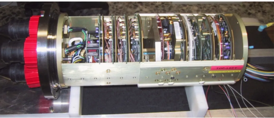
323
2.3. Detector design considerations
324
The detector location on the seabed at a depth of 2475 m imposes many
325
constraints on the detector design. All components must withstand a
hydro-326
static pressure between 200 and 256 bar and resist corrosion or degradation
327
in the sea water of 46 mS cm−1 conductivity. The seabed environment has
328
a stable temperature around 13 ◦C and little risk of shock or variable
me-329
chanical stress. The detector lines sway in the sea current which is typically
10 cm s−1 with variations up to a maximum value of 30 cm s−1. The detector
331
components were designed to take into account possible shocks, vibrations
332
and high temperatures during construction, transport and deployment. All
333
components were chosen with the objective of a minimum detector life time
334
of 10 years.
335
The materials to be in contact with the sea water were selected
accord-336
ing to their known resistance to corrosion: glass, titanium alloys (grade
337
2 and 5), anode protected carbon steel, polyethylene (LDPE and PETP),
338
polyurethane, aramid and glass-epoxy (syntactic foam and fibre composite).
339
Stainless steel and aluminium alloys were not used due to their reduced
cor-340
rosion resistance. In addition to this material selection, special attention was
341
paid to prevent any parasitic electrical currents able to induce electrolytic
342
corrosion. Isolating interfaces were used between metals of different nature
343
and the electrical power distribution system was designed to prevent any
344
current leak to the water.
345
Avoiding water leaks during operation imposed many constraints on the
346
detector design. When possible, O-rings in containers, made of Viton8 or
347
nitrile material were implemented in two seals in a redundant way. The
348
O-ring material hardness, its cross section diameter, the shape and the
sur-349
face roughness of the groove as well as the characteristics of the matching
350
parts were specified following the recommendations of the manufacturer for
351
the in situ pressure. Tests under pressure were performed on all the major
352
containers (JB container and glass spheres) and EMC sections.
Electron-353
ics containers have been tested by sampling. Some tests were performed by
354
the manufacturer of the component (glass spheres and short sections of the
355
EMC ) and others were performed by the collaboration at IFREMER9, at
356
the COMEX10 and Ring-O Valve11 companies (JB and electronics
contain-357
ers, the rest of the EMC sections). The pressure tests were based on the
358
IFREMER rules for undersea vessels for a working pressure of 256 bar: a
359
cycle up to 310 bar for 24 h and ten cycles up to 256 bar for 1h with all the
360
pressure changes made at a rate of ± 12 bar per minute. The criterion of
361
success for the acceptance test was the integrity of the tested element, the
362
absence of water inside the containers and the electro-optical continuity of
363
8
Vitonr, http://www.dupontelastomers.com/products/viton/ 9IFREMER, www.ifremer.fr
10COMEX, www.comex.fr
the cable under static pressure conditions.
364
The maximum static tension along the line is expected to occur during
365
the line deployment in the section below the first storey, which has to sustain
366
the weight in water of the full anchor (BSS + deadweight): ≈ 3 tons.
Dy-367
namic load may reach higher values during the deployment, due to the swell.
368
Since the total mass of the line is 7 tons, an upward acceleration of 1 g, for
369
instance, will add a tension of 70 kN in the top part of the line during the
370
descent. In order to minimise the risks of high dynamic loads, the
deploy-371
ment of the lines were required to be performed in quiet sea state (≤ 3 on
372
the Beaufort scale, corresponding to waves of ≈ 60 cm high). However, since
373
the conditions are difficult to predict accurately for the ≈ 8 hours needed for
374
a deployment or a recovery, the general dimensioning rules recommended by
375
IFREMER for deployments in the sea from a surface boat were imposed:
376
Breaking Load > Static Load × A (1)
where A = 1.5 for metal parts (BSS, OMF and buoy equipment) and 4 for
377
organic fibres (the Aramid braid of the vertical EMC). This rule results in a
378
breaking load of more than 7 tons for the OMF and 18 tons for the EMC.
379
3. Line structure
380
A line is the assembly of an anchor sitting on the seabed, 25 storeys and
381
a top buoy linked by electro-optical mechanical cables. A storey consists of
382
three optical modules, the metal structure that supports them and provides
383
interfaces with the EMCs, the electronics container and additional
instru-384
mentation. In order to limit the number of single point failures for a full
385
line, a line is divided in 5 sectors of 5 successive storeys each. The sectors
386
are independent for the power distribution and the data transmission. The
387
distribution of power and routing of clock and acquisition signals toward each
388
sector are performed in electronics containers fixed on the BSS.
389
3.1. Optical modules
390
The optical module, the basic sensor element of the telescope, is the
391
assembly of a pressure resistant glass sphere housing a photomultiplier tube,
392
its base and other components. A detailed description of the ANTARES OM
393
can be found in [10].
3.1.1. Photo detector requirements
395
The search for a highly sensitive light detector led to the choice of
pho-396
tomultiplier tubes with a photocathode area as large as possible combined
397
with a large angular acceptance. Regarding these criteria, the best
candi-398
dates are large hemispherical tubes. However, the PMT size is limited by
399
some characteristics which increase with the photocathode area:
400
- the transit time spread (TTS) which has to be small enough to ensure
401
the required time resolution,
402
- the dark count rate which must be negligible compared to photon
back-403
ground rate.
404
In summary, the main requirements for the choice of the ANTARES
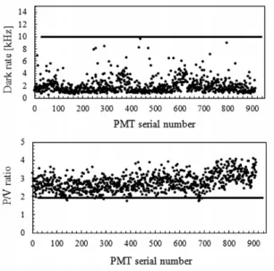
405 PMTs are: 406 ◦ photocathode area > 500 cm2 407 ◦ quantum efficiency > 20 % 408 ◦ collection efficiency > 80% 409 ◦ TTS < 3 ns 410
◦ dark count rate < 10 kHz (threshold at 1/3 SPE, including glass
411
sphere)
412
◦ peak/valley ratio > 2
413
◦ peak width (FWHM)/peak position < 50%
414
◦ gain of 5×10⁷ reached with HV < 2000 V
415
◦ pre-pulse rate < 1%
416
◦ after-pulse rate < 15%
417
3.1.2. Optical module components
418
Figure 4 shows a schematic view of an optical module with its main
419
components. The following sections describe the different components and,
420
when relevant, the assembly process.
421
3.1.2.1. Photomultiplier tube.
422
In the R&D phase, an extensive series of tests were performed on several
423
commercially available models of large hemispherical photomultipliers. A
424
summary of this study is presented in [11]. The R7081-20, a 10”
hemispheri-425
cal tube from Hamamatsu12, was chosen. The full sample of delivered PMTs
426
has been tested with a dedicated test bench in order to calibrate the sensors
427
and to check the compliance with the specifications. The number of rejected
428
Figure 4: Schematic view of an optical module
tubes was small (17, their peak/valley ratio being too low), these tubes were
429
replaced by the manufacturer. To illustrate the homogeneity of the
produc-430
tion, Figure 5 shows the measured values of dark noise rate (top) and of the
431
peak/valley ratio (bottom). During the testing process, the working point of
Figure 5: Results of dark count rate (top) and peak/valley ratio (bottom) for the full set of tested PMTs.
432
each PMT, i.e. the high voltage needed to obtain a gain of 5 × 10⁷ ± 10 %,
433
was determined by measuring the value of the SPE pulse height. The results
of these measurements are illustrated in Figure 6.
Figure 6: Measured mean pulse height of single photoelectrons for each PMT at nominal gain.
435
3.1.2.2. Glass sphere.
436
The protective envelope of the PMT is a glass sphere of a type
rou-437
tinely used by sea scientists for buoyancy and for instrument housing. These
438
spheres, because of their mechanical resistance to a compressive stress and of
439
their transparency, provide a convenient housing for the photodetectors.
Ta-440
ble 1 summarizes the main characteristics of the Vitrovexr glass spheres13
441
used. The sphere is provided as two hemispheres: one, referred to as “back
Outer diameter 432 mm (17”)
Wall thickness 15 mm
Type of glass Borosilicate
Refractive index 1.47
Light transmission above 350 nm >95%
Density 2.23 g cm−3
Pressure of qualification test 700 bar (70 MPa) Diameter shrinking at 250 bar 1.25 mm (0.3%) Absolute internal air pressure 0.7 bar (70 kPa)
Hole diameters 20 mm, 5 mm
(penetrator and vacuum port)
Table 1: Data on the OM glass sphere.
442
hemisphere” is painted black on its internal surface and the other, “front
443
hemisphere” is transparent. The front hemisphere houses the PMT and the
444
magnetic shielding held in place by the optical gel. The back hemisphere
445
has two drilled holes to accommodate the electrical connection via a
pene-446
trator and a vacuum port. Around both holes a flat surface is machined on
447
the outside of the sphere for the contact of the single O-ring ensuring water
448
tightness. The back hemisphere is also equipped with a manometer readable
449
from the outside. The two glass halves have precisely machined flat
equato-450
rial surfaces in direct contact (glass/glass) without any gasket or interface.
451
The risk of implosion and the consequences on the structure were
consid-452
ered since its potential energy is of the order of a megajoule (200 g of TNT)
453
at the depth of the detector. Based on tests performed by DUMAND [12]
454
and further tests performed off Corsica in the year 2000 by the ANTARES
455
Collaboration, it has been concluded that the implosion of a glass sphere at
456
the ANTARES depth would provoke the loss of the two other spheres of the
457
same storey (at centre distances of 770 mm) but not of spheres on adjacent
458
storeys (at a distance of 14.5 m), and would not cut or damage the cable.
459
The rigid storey mechanical frame would be distorted but not destroyed by
460
the implosion.
461
3.1.2.3. Optical gel.
462
The optical coupling between the glass sphere and the PMT is achieved
463
with optical gel. The chosen gel is a two-component silicon rubber provided
464
by the Wacker company14. The mixture of the components is made in the
465
ratio 100:60. After curing and polymerization, lasting 4 hours at ambient
466
temperature, the optical gel reaches an elastic consistency soft enough to
467
absorb the sphere diameter reduction by the deep sea pressure (1.2 mm)
468
and stiff enough to hold the PMT in position in the sphere. The optical
469
properties of the gel have been measured in the laboratory: the absorption
470
length is 60 cm and the refractive index is 1.404 for wavelengths in the blue
471
domain.
472
3.1.2.4. Magnetic shield.
473
At the ANTARES site, the Earth’s magnetic field has a magnitude of
474
approximately 46 µT and points downward at 31.5◦ from the vertical.
Un-475
corrected, the effect of this field would be a significant degradation of the
476
TTS, of the collection efficiency and of the charge amplification of the PMT.
477
A magnetic shield is implemented by surrounding the bulb of the PMT with
478
a hemispherical grid made of wires of µ-metal15 closed by a flat grid on the
479
rear of the bulb. This provides a magnetic shielding for the collection space
480
and for the first stages of the amplification cascade. The efficiency of the
481
screening becomes larger as the size of the mesh is reduced and/or the wire
482
diameter is increased, however the drawback is a shadowing effect on the
483
photocathode. The compromise adopted by the ANTARES Collaboration, a
484
mesh of 68 × 68 mm2 and wire diameter of 1.08 mm, results in a shadowing
485
of less than 4 % of the photocathode area while reducing the magnetic field
486
by a factor of three. Measurements performed in the laboratory show that
487
this shielding provides a reduction of 0.5 ns on the TTS and a 7 % increase
488
on the collected charge with respect to a naked, uniformly illuminated PMT.
489
3.1.2.5. HV power supply.
490
To limit the power consumption of the HV power supply a high voltage
491
generator based on the Cockroft-Walton [13] scheme is adopted. The HV
492
generator chosen for the ANTARES detector is derived from the model
de-493
veloped for the AMANDA experiment16, and is manufactured by the iseg
494
company17. It has two independent high-voltage chains. The first chain
495
produces a constant focusing voltage (800 V) to be applied between
photo-496
cathode and first dynode. The second chain gives the amplification voltage,
497
which can be adjusted from 400 V to 1600 V by an external DC voltage.
498
The HV generator is powered by a 48 V DC power supply and has a typical
499
consumption of 300 mW.
500
The signals of the anode, of the last dynode and of the last-but-two
dyn-501
ode of the PMT are routed to the electronics container together with the
502
PMT ground. A low level voltage image of the actual HV is provided for
503
monitoring purpose.
504
3.1.2.6. Internal LED.
505
On the rear part of the bulb of the PMT, a blue LED is glued in such
506
a way to illuminate the pole of the photocathode through the aluminium
507
15Sprint Metal, Ugitech, http://www.ugitech.com 16http://icecube.wisc.edu/
coating, which acts as a filter of large optical density (optical density ≈ 5).
508
This LED is excited by an externally driven pulser circuit and is used to
509
monitor the internal timing of the OM.
510
3.1.2.7. Link with the electronics container.
511
The electrical connection of the OM to the electronics container is made
512
with a penetrator18 (Ti socket with polyurethane over moulding). The
as-513
sociated cable contains shielded twisted pairs for the transmission of power,
514
the control of the LED pulser and the setting and monitoring of the DC
515
command voltage of the PMT base. One pair is used to transmit the
an-516
ode and the last dynode signals. This pseudo differential transmission pair
517
has the advantage of reducing the noise and enhancing the output signal by
518
approximately a factor of two when the subtraction is done at the readout
519
electronics. The last pair is used to transmit signals from the last-but-two
520
dynode, together with the ground, for the treatment of very high amplitude
521
signals.
522
3.1.2.8. Final assembly and tests.
523
The assembly starts with the pouring of the gel into the front hemisphere
524
and a precise sequence of out-gasing is applied in order to avoid the
appear-525
ance of bubbles during the polymerization phase. Then, the cage and the
526
PMT are positioned by tools which ensure a defined position with respect
527
to marks on the hemisphere. These marks are also used to mount the OM
528
on its support structure, giving each PMT a well-defined and reproducible
529
orientation with respect to the storey mechanical structure.
530
After the gluing of the LED, the cabling of the base to the pig-tail of the
531
penetrator and the connection of the PMT, the back hemisphere is placed
532
in contact with the front one. Closure is obtained by establishing an
un-533
derpressure of ≈ 300 mbar inside the sphere. The equatorial seam is sealed
534
externally with butyl rubber sealant which is protected by a sealant tape.
535
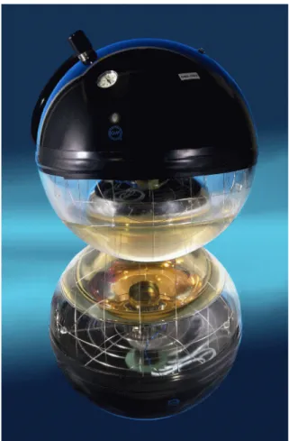
Figure 7 shows an assembled OM. The same test bench as for the naked
536
PMT is used to test the OM. Dark count rate, gain and LED functionality
537
are checked.
538
18EurOc´eanique S.A., part of MacArtney Underwater Technology, http://www.macartney.com
Figure 7: Photograph of an optical module. It is positioned on a mirror to better show the full assembly.
3.1.3. OM support
539
The OM support is made of a stamped Ti grade 2 conical plate (OD = 280 mm)
540
on which the OM is pulled by a pair of Ti wires ( = 4 mm) under tension
541
running around the glass sphere (Figure 8). The wires are designed to follow
542
a great circle of the sphere, which results in their stable equilibrium position
543
on the glass surface. A set of 5 rubber pads are inserted between the metal
544
parts and the OM to protect the glass surface and to keep the assembly under
545
tension in spite of the pressure shrinking. Tests at 250 bar (25 MPa) showed
546
that the support allows the OM to sustain a test torque of 5 Nm without
547
rotating. The titanium plate is also the interface to the optical module frame.
Figure 8: OM support mechanics.
3.2. Storey
549
3.2.1. Optical module frame
550
The role of the optical module frame (OMF) is to hold the three OMs
551
of the storey, the associated LCM container and to connect both mechanical
552
terminations of the EMCs. The OMF and its connections are specified up
553
to a breaking load of 7 tons. Some OMFs also hold optional equipment such
554
as LED beacons [14], positioning hydrophones and certain oceanographic
555
sensors.
556
The OMF (Figure 9) is a welded vertical structure of Ti (grade 2; chosen
557
for the ease of welding) and of three-fold periodic symmetry around the
558
vertical axis. The main elements are:
559
• at the top and bottom, two rings (ID = 85 mm) on which are locked
560
the EMC mechanical terminations;
561
• three shaped tubes (OD = 33.4 mm, thickness = 3.38 mm) connecting
562
these rings vertically with an overall height of 2.12 m (2 m between
563
EMC mechanical terminations);
564
• four spacers of triangular shape made of 12 mm diameter rod between
565
the three tubes:
566
– the bottom triangle holds the LCM container on the vertical axis
567
of the OMF;
568
– the next spacer stiffens the structure at the height of the 3 OM
569
fixture plates (80×80×5 mm), welded on each tube at a distance
570
of 195 mm from the axis;
Figure 9: OMF equipped with the 3 OMs, the LCM and an LED beacon. The mechanical parts used for fixing cables toward the upper and the lower storeys are omitted.
– the two top spacers are used to hold the optional LED beacon.
572
All OMFs were validated by applying a traction load of 80 kN, which is
573
in fact higher than the load resulting from the design rule of 7 tons.
574
3.2.2. Local control module
575
3.2.2.1. Container.
576
The housing of the readout electronics is a Ti grade 5 container made
577
of a hollow cylinder (600 mm long, 179 mm outer diameter and 22 mm
578
wall thickness) closed by two end caps (30 mm thick). The top end cap
579
accommodates the two large penetrators of the EMC linking the storey to
580
its upper and lower adjacent storey. The bottom end cap accommodates
581
three connectors linking the LCM to its three optical modules. In some of
582
the LCMs, a 4th connector is needed for additional equipment. The fixation
583
of the end caps on the cylinder and of the whole container on the OMF is
made with three external threaded rods of 6 mm diameter in Ti grade 2.
585
The thickness of the cylinder and of the end-caps was optimised by Finite
586
Element Method analysis with the goal to stay within the yield strength
587
of the material at an external pressure of 310 bars. The calculations were
588
tested by the collapse under pressure of an Al alloy container of the same
589
configuration. Ti grade 5 was chosen for its yield strength around 900 MPa,
590
compared to that of grade 2 which is around 300 MPa.
591
3.2.2.2. Electronics.
592
In order to optimally fill the cylindrical volume offered by the container,
593
a dedicated crate was developed. This crate accepts circular shaped printed
594
circuit boards plugged on a backplane which distributes the signals as well
595
as the DC power supplied by the local power box. The crate was designed
596
to ensure that its mechanical structure acts as a medium that transfers the
597
heat produced by the electronics to the Ti cylinder in contact with the water.
598
After evaluating different metals, the final choice was made for aluminium
599
which can guarantee good performance with light weight and at an affordable
600
price. Furthermore, boards having high power consumption are equipped
601
with metal cooling bases which are in thermal contact with the crate.
602
Most of the LCMs contain the same set of electronics cards. However, due
603
to the segmentation of a line in sectors, one in five LCMs, called Master LCM
604
or MLCM, acts as a master for other LCMs of the same sector and houses
605
additional boards. Other differences between individual LCMs are due to
606
electronics necessary for optional equipment on the storey (hydrophone, LED
607
beacon, ...).
608
A standard LCM contains the following elements:
609
• LPB. Fixed on the crate, the local power box is fed by the 400 V DC
610
from the bottom of the line, and provides the 48 V for the optical
611
modules and several different low voltages for the electronics boards.
612
An embedded micro-controller allows the monitoring of the voltages,
613
the temperatures and the current consumptions as well as the remote
614
setting of the 48 V for the OMs.
615
• CLOCK. The clock reference signal coming from shore reaches the
bot-616
tom of the line where it is repeated and sent to each sector. Within
617
a sector, the clock signal is daisy-chained between LCMs. The role of
618
the CLOCK card is to receive the clock signal from the lower LCM,
619
to distribute it on the backplane and to repeat it toward the upper
LCM of the sector. It also has the capability to pass commands on the
621
backplane which are coded within the clock signal.
622
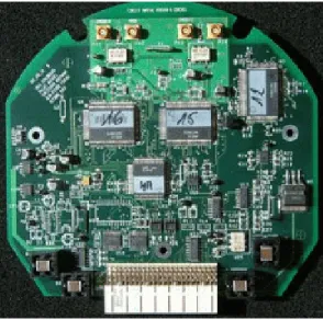
• ARS MB (Figure 10). The ARS motherboards host the front-end
elec-623
tronics of the OMs (one board per OM). This front-end electronics
con-624
sists of a custom-built Analogue Ring Sampler (ARS) chip [9] which
Figure 10: The ARS MB board with the 2 ARSs (labelled 16 and 15). The 3rd one (top right, labelled 12) is foreseen for trigger purposes.
625
digitizes the charge and the time of the analogue signal coming from
626
the PMTs, provided its amplitude is larger than a given threshold.
627
The level of this threshold is tuneable by slow-control commands. The
628
analogue signal is integrated by an AVC (Amplitude to Voltage
Con-629
verter) to obtain the charge which is digitized by an ADC. The ARS
630
can also operate like a flash-ADC using analog memories with a
sam-631
pling tuneable down to sub-nanosecond values. The output consists of
632
a waveform of 128 amplitude samples. The arrival time is determined
633
from the signal of the clock system in the LCM and from a TVC (Time
634
to Voltage Converter) which provides a sub-nanosecond resolution. To
635
minimise the dead time induced by the digitization, each ARS MB card
636
is equipped with 2 ARSs working in a token ring scheme. For a storey
637
with an optical beacon, a 4thARS MB is installed to digitize the signals
638
sent by the internal PMT of the beacon.
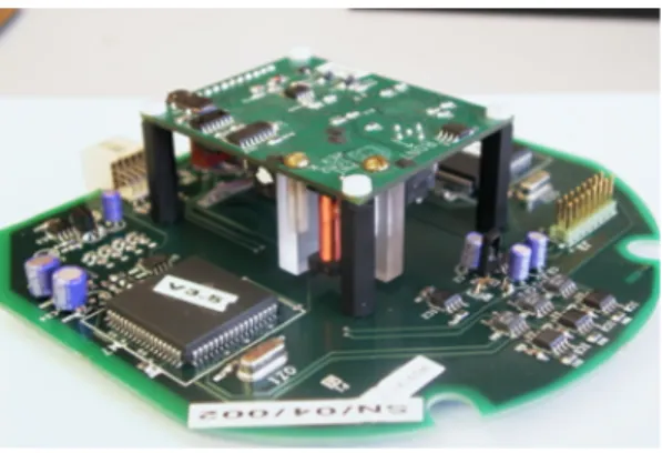
• DAQ/SC (Figure 11). The DAQ/Slow-Control card host the local
pro-640
cessor and memory. The processor is a Motorola MPC860P which
641
runs the VxWorks real time operating system19 and hosts the software
642
processes [8]. These processes are used to handle the data from the
643
ARS chips and from the slow control, respectively. The processor has
644
a fast Ethernet controller (100 Mb s−1) that is optically connected to
645
an Ethernet switch in the MLCM of the corresponding sector. Three
Figure 11: The DAQ/SC board holding the processor (centre), the FPGA (left) and the optical link to the MLCM (right).
646
serial ports, two with RS485 links and one with RS232 links, using the
647
MODBUS protocol20 are used to handle the slow control signals. The
648
specific hardware for the readout of the ARS chips and data
format-649
ing is implemented in a high density field programmable gate array21.
650
The data are temporarily stored in a high capacity memory (64 MB
651
SDRAM) allowing a de-randomisation of the data flow.
652
• COMPASS MB (Figure 12). The compass motherboard hosts a TCM22
653
sensor which provides heading, pitch and roll of the LCM (i.e. of the
654
19Wind River, http://www.windriver.com 20http://www.modbus.org
21Virtex-EXCV1000E, http://www.xilinx.com 22PNI Sensor Corp., http://www.pnicorp.com
OMF) used for the reconstruction of the line shape and PMT positions.
655
The heading is measured with an accuracy of 1◦ over the full cycle and
656
the tilts with an accuracy of 0.2◦ over a range of ±20◦. The same
657
card supports two micro-controllers dedicated to the slow control: they
658
control the measurements of various temperatures and the humidity,
659
and set and monitor the PMT high voltages.
Figure 12: The COMPASS MB equipped with a TCM2 sensor on a raised daughter card.
660
For LCMs performing acoustic functions (cf. Section 3.8), there are three
661
additional cards: one housing a pre-amplifier, one a CPU and the third a
662
digital signal processor. These cards are commercial products from ECA23,
663
re-shaped to fit in the crate.
664
An MLCM holds the following additional cards:
665
• BIDICON. It communicates via bi-directional optical fibres with the
666
four other LCMs of the sector, and performs the electrical↔optical
con-667
version of signals transmitted via the backplane to or from the SWITCH
668
card.
669
• SWITCH. An Ethernet switch which consists of a combination of eight
670
100 Mb s−1ports and two 1 Gb s−1ports24. One of the 100 Mb s−1ports
671
is connected to the processor of the MLCM and four to the BIDICON
672
card via the backplane. One of the two Gb s−1 ports is connected to a
673
Dense Wavelength (De)-Multiplexer (DWDM) transceiver.
674
23ECA S.A., http://www.eca.fr
• DWDM (Figure 13). The role of the transceiver is to perform the
675
electrical↔optical conversion for the full sector and to communicate
676
with the shore via the SCM located at the bottom of the line. It
677
is electrically connected to the SWITCH card via coaxial cables and
678
optically to the SCM via two uni-directional optical fibres (Rx and Tx)
679
at a connection speed of 1 Gb s−1. For each MLCM (i.e. sector) of a
680
line, the laser mounted on the card has a specific frequency chosen in
681
the range from 192.1 to 194.9 THz, the frequency spacing being 400
682
GHz.
Figure 13: The DWDM board.
683
Figure 14 shows an MLCM crate equipped with the full set of the
elec-684
tronics cards. A description of the components in the SPM/SCM container
685
will be given later in the BSS Section 3.4.3.
686
3.3. Electro-optical mechanical cable (EMC)
687
The EMC cable has three roles:
688
• optical data link: 21 single mode optical fibres ( =9/125/250 µm) run
689
along the cable;
690
• power distribution: 9 electrical conductors (Cu section = 1 mm2 with
691
insulation = 2.5 mm);
692
• mechanical link: breaking tension above 177 kN.
Figure 14: The crate of an MLCM equipped with the electronics boards.
To facilitate the line handling and deployment with its cumulative length
694
of ≈ 480 m, the minimal allowed radius of curvature of the cable was specified
695
to be less than 300 mm (180 mm for the naked core).
696
The cable, developed under the responsibility of EurOc´eanique18is
assem-697
bled in successive layers as shown in Figure 15. The two internal layers are
ARAMID BRAID FILLING BODY CONDUCTOR FIBRE TUBE PU LDPE
Figure 15: Cross section of the EMC. From centre to outside one can distinguish the layer with 3 tubes, each housing 7 optical fibres, the layer with 9 copper conductors, the LDPE jacket, the aramid braid and the polyurethane sheath. The external diameter is 30 mm.
698
assembled with silicon compound filling the space between the elements.
Wa-699
ter can penetrate through the 2 external layers, while the inner polyethylene
700
jacket acts as a water barrier. The polyurethane (PU) sheath is in contact
with the water. Its role is to protect the aramid braid and the cable
be-702
fore and during deployment. The two outer layers end inside the mechanical
703
termination where the aramid braid is firmly held by a cone locking-system
704
and the rest of the cable, called the “core”, continues for a few meters to
705
the LCM penetrators. Each section sustained a static test tension of 50 kN.
706
During this test, the insulation of electrical conductors and the attenuation
707
on the optical fibres are controlled. The cable length between the mechanical
708
terminations is 98 m for the bottom cable section and 12.5 m for the 25 other
709
sections of a line (including the passive section linking the top storey to the
710
buoy), resulting in a pitch between optical modules of 14.5 m. The actual
711
length of each section delivered was measured under a tension of one ton,
712
with an accuracy of ±5 mm, and the results were recorded in a database as
713
input to the line shape reconstruction. Figure 16 gives a schematic view of
714
the top and bottom mechanical terminations and their PU bending limitors.
715 TOP BOTTOM EMC Core Bending limitor (PU) Locking groove Core EMC
holding pointDeployment hook (PU) Bending limitor Locking groove
Figure 16: Mechanical termination of an EMC.
716
Two different types of LCM penetrators are mounted at the ends of the
717
core: a pair of water-blocking (WB) penetrators for the sections located
718
between sectors and a less expensive pair of non-water-blocking (NWB)
etrators elsewhere. In case of a flooded cable, the WB type stops the
prop-720
agation of the water along the cable and thus limits the flooded part of the
721
line to one sector (the WB penetrator only stops water propagation from the
722
cable to the container and not in the opposite direction). Figure 17 gives
723
a schematic view of the NWB penetrator (left) and of the WB penetrator
724
(right). In both cases, the fibre tubes are mechanically blocked in an epoxy
725
moulding, itself blocked in the penetrator body to avoid extrusion when the
726
cable is subject to water pressure.
Figure 17: EMC penetrators of the LCM container. Left: non water blocking. Right: water blocking. For clarity, the 3rd fibre tube and the 9 conductors are not shown.
727
When subjectted to a uniform horizontal sea current, as present at the
728
ANTARES site, the 3-fold periodic symmetry of the storey induces a torque
729
which is a function of the actual azimuth of the storey. The storey is in stable
730
equilibrium when one of the three OMs is upstream of the current. From
731
measurements performed in a pool, the torque was found to be proportional
732
to the square of the current with a proportionality constant of 9.47 N s2 m−1.
733
Between two adjacent storeys, the EMC acts as a torsion spring tending to
734
keep them at the same relative angle. This torque was measured as a function
735
of the cable tension on a prototype and found to be proportional to the
736
cable torsion angle per unit length and to the tension with a proportionality
737
constant of 1.3 × 10⁻³ m2 rad−1. In order to specify the minimum torsion
738
strength of the cable, the torsion behaviour of the line was simulated using
739
the above data and for very unfavorable environmental conditions: uniform