A benchmark study on the thermal conductivity of nanofluids
The MIT Faculty has made this article openly available.
Please share
how this access benefits you. Your story matters.
Citation
Buongiorno, Jacopo et al. “A benchmark study on the thermal
conductivity of nanofluids.” Journal of Applied Physics 106 (2009):
094312. Copyright © 2009, American Institute of Physics
As Published
http://dx.doi.org/10.1063/1.3245330
Publisher
American Institute of Physics
Version
Final published version
Citable link
http://hdl.handle.net/1721.1/66196
Terms of Use
Article is made available in accordance with the publisher's
policy and may be subject to US copyright law. Please refer to the
publisher's site for terms of use.
A benchmark study on the thermal conductivity of nanofluids
Jacopo Buongiorno,1,a兲 David C. Venerus,2Naveen Prabhat,1Thomas McKrell,1 Jessica Townsend,3Rebecca Christianson,3 Yuriy V. Tolmachev,4Pawel Keblinski,5 Lin-wen Hu,1Jorge L. Alvarado,6In Cheol Bang,7,8Sandra W. Bishnoi,2Marco Bonetti,9 Frank Botz,10Anselmo Cecere,11Yun Chang,12Gang Chen,1Haisheng Chen,13
Sung Jae Chung,14Minking K. Chyu,14Sarit K. Das,15Roberto Di Paola,11Yulong Ding,13 Frank Dubois,16Grzegorz Dzido,17Jacob Eapen,18Werner Escher,19,20
Denis Funfschilling,21Quentin Galand,16Jinwei Gao,1Patricia E. Gharagozloo,22 Kenneth E. Goodson,22 Jorge Gustavo Gutierrez,23 Haiping Hong,24 Mark Horton,24 Kyo Sik Hwang,25Carlo S. Iorio,16Seok Pil Jang,25Andrzej B. Jarzebski,17Yiran Jiang,2 Liwen Jin,26 Stephan Kabelac,27 Aravind Kamath,6 Mark A. Kedzierski,28
Lim Geok Kieng,29Chongyoup Kim,30Ji-Hyun Kim,7Seokwon Kim,30Seung Hyun Lee,25 Kai Choong Leong,26Indranil Manna,31Bruno Michel,19Rui Ni,21Hrishikesh E. Patel,15 John Philip,32 Dimos Poulikakos,20 Cecile Reynaud,9 Raffaele Savino,11
Pawan K. Singh,15Pengxiang Song,33Thirumalachari Sundararajan,15Elena Timofeeva,34 Todd Tritcak,10Aleksandr N. Turanov,4Stefan Van Vaerenbergh,16Dongsheng Wen,33 Sanjeeva Witharana,13Chun Yang,26Wei-Hsun Yeh,2Xiao-Zheng Zhao,21and Sheng-Qi Zhou21
1
Massachusetts Institute of Technology (MIT), 77 Massachusetts Avenue, Cambridge, Massachusetts 02139, USA
2
Illinois Institute of Technology, 10 W. 33rd St., Chicago, Illinois 6016, USA 3
Olin College of Engineering, Olin Way, Needham, Massachusetts 02492, USA 4
Kent State University, Williams Hall, Kent, Ohio 44242, USA 5
Materials Research Center, Rensselaer Polytechnic Institute (RPI), 110 8th Street, Troy, New York 12180, USA
6
Texas A&M University, MS 3367, College Station, Texas 77843, USA 7
School of Energy Engineering, Ulsan National Institute of Science and Technology, San 194 Banyeon-ri, Eonyang-eup, Ulju-gun, Ulsan Metropolitan City, Republic of Korea
8
Tokyo Institute of Technology, 2-12-1 Ookayama, Meguro-ku, Tokyo 152-8550, Japan 9
Commissariat à l’Énergie Atomique (CEA), IRAMIS, 91191 Gif sur Yvette, France 10
METSS Corporation, 300 Westdale Avenue, Westerville, Ohio 43082, USA 11
Department of Aerospace Engineering, University of Naples, P.le V. Tecchio 80, 80125 Naples, Italy 12
SASOL of North America, 2201 Old Spanish Trail, Westlake, Louisiana 70669-0727, USA 13
University of Leeds, Clarendon Road, Leeds LS2 9JT, United Kingdom
14Department of Mechanical Engineering and Materials Science, University of Pittsburgh, 648 Benedum Hall, 3700 O’Hara Street, Pittsburgh, Pennsylvania 15261, USA
15Department of Mechanical Engineering, Indian Institute of Technology-Madras, Chennai 600036, India 16Université Libre de Bruxelles, Chimie-Physique E.P. CP 165/62 Avenue P.Heger, Bat. UD3,
Bruxelles 1050, Belgium
17Department of Chemical and Processing Engineering, Silesian University of Technology, ul. M. Strzody 7, 44-100 Gliwice, Poland
18
Department of Nuclear Engineering, North Carolina State University, Raleigh, North Carolina 27695-7909, USA
19
Zurich Research Laboratory, IBM Research GmbH, Saeumerstr. 4, CH-8803 Rüschlikon, Switzerland 20
Department of Mechanical and Process Engineering, Laboratory of Thermodynamics in Emerging Technologies, ETH Zurich, 8092 Zurich, Switzerland
21
Department of Physics, Chinese University of Hong Kong, G6, North Block, Science Center, Shatin NT, Hong Kong, China
22
Stanford University, 440 Escondido Mall Rm 224, Stanford, California 94305, USA 23
Department of Mechanical Engineering, University of Puerto Rico-Mayaguez, 259 Boulevard Alfonso Valdes, Mayaguez 00681, Puerto Rico
24
South Dakota School of Mines and Technology, 501 E Saint Joseph Street, Rapid City, South Dakota 57701, USA
25
School of Aerospace & Mechanical Engineering, Korea Aerospace University, 100, Hwajeon-dong, Deogyang-gu, Goyang-city, Gyeonggi-do 412-791, Republic of Korea
26
School of Mechanical and Aerospace Engineering, Nanyang Technological University, 50 Nanyang Avenue, Singapore 639798, Singapore
27
Institute for Thermodynamics, Helmut-Schmidt University Hamburg, D-22039 Hamburg, Germany 28
National Institute of Standards and Technology (NIST), MS 863, Gaithersburg, Maryland 20899, USA 29
DSO National Laboratories, 20 Science Park Drive, Singapore 118230, Singapore 30
Korea University, Anam-dong, Sungbuk-ku, Seoul 136-713, Republic of Korea 31
Department of Metallurgical and Materials Engineering, Indian Institute of Technology-Kharagpur, West Bengal 721302, India
a兲Author to whom correspondence should be addressed. Electronic mail: [email protected]. Tel.:⫹1共617兲253-7316.
32
SMARTS, NDED, Metallurgy and Materials Group, Indira Gandhi Centre for Atomic Research, Kalpakkam 603102, India
33
School of Engineering and Materials Science, Queen Mary University of London, Mile End Road, London E1 4NS, United Kingdom
34
Argonne National Laboratory, 9700 S. Cass Avenue, Argonne, Illinois 60439, USA
共Received 12 June 2009; accepted 6 September 2009; published online 13 November 2009兲 This article reports on the International Nanofluid Property Benchmark Exercise, or INPBE, in which the thermal conductivity of identical samples of colloidally stable dispersions of nanoparticles or “nanofluids,” was measured by over 30 organizations worldwide, using a variety of experimental approaches, including the transient hot wire method, steady-state methods, and optical methods. The nanofluids tested in the exercise were comprised of aqueous and nonaqueous basefluids, metal and metal oxide particles, near-spherical and elongated particles, at low and high particle concentrations. The data analysis reveals that the data from most organizations lie within a relatively narrow band共⫾10% or less兲 about the sample average with only few outliers. The thermal conductivity of the nanofluids was found to increase with particle concentration and aspect ratio, as expected from classical theory. There are共small兲 systematic differences in the absolute values of the nanofluid thermal conductivity among the various experimental approaches; however, such differences tend to disappear when the data are normalized to the measured thermal conductivity of the basefluid. The effective medium theory developed for dispersed particles by Maxwell in 1881 and recently generalized by Nan et al.关J. Appl. Phys. 81, 6692 共1997兲兴, was found to be in good agreement with the experimental data, suggesting that no anomalous enhancement of thermal conductivity was achieved in the nanofluids tested in this exercise. © 2009 American Institute of
Physics.关doi:10.1063/1.3245330兴
I. INTRODUCTION
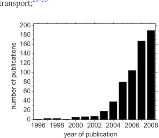
Engineered suspensions of nanoparticles in liquids, known recently as “nanofluids,” have generated considerable interest for their potential to enhance the heat transfer rate in engineering systems, while reducing, or possibly eliminating, the issues of erosion, sedimentation and clogging that plagued earlier solid-liquid mixtures with larger particles. According to SciFinder Scholar, in 2008 alone 189 nanofluid-related publications 共journal articles and patents兲 appeared共see Fig.1兲, and it is estimated that more than 300 research groups and companies are engaged in nanofluids research worldwide. Furthermore, several review papers on nanofluid heat transfer have been published1–7 and recently even a book entirely dedicated to nanofluids has been released.8
In spite of the attention received by this field, uncertain-ties concerning the fundamental effects of nanoparticles on thermophysical properties of solvent media remain. Thermal conductivity is the property that has catalyzed the attention of the nanofluids research community the most. As disper-sions of solid particles in a continuous liquid matrix, nano-fluids are expected to have a thermal conductivity that obeys the effective medium theory developed by Maxwell over 100 years ago.9 Maxwell’s model for spherical and well-dispersed particles culminates in a simple equation giving the ratio of the nanofluid thermal conductivity 共k兲 to the thermal conductivity of the basefluid共kf兲
k kf
=kp+ 2kf+ 2共kp− kf兲
kp+ 2kf−共kp− kf兲
, 共1兲
where kp is the particle thermal conductivity and is the
particle volumetric fraction. Note that the model predicts no explicit dependence of the nanofluid thermal conductivity on
the particle size or temperature. Also, in the limit of kpⰇkf
andⰆ1, the dependence on particle loading is expected to be linear, as given by k/kf⬇1+3. However, several
devia-tions from the predicdevia-tions of Maxwell’s model have been reported, including:
• a strong thermal conductivity enhancement beyond that predicted by Eq.共1兲with a nonlinear dependence on particle loading;10–16
• a dependence of the thermal conductivity enhancement on particle size and shape; and15,17–25
• a dependence of the thermal conductivity enhancement on fluid temperature.20,26–28
To explain these unexpected and intriguing findings, sev-eral hypotheses were recently formulated. For example, it was proposed that:
• particle Brownian motion agitates the fluid, thus creat-ing a microconvection effect that increases energy transport;29–33 1996 1998 2000 2002 2004 2006 2008 0 20 40 60 80 100 120 140 160 180 200 number of pu blicat ions year of publication
FIG. 1. Number of publications containing the term nanofluid according to SciFinder Scholar.
• clusters or agglomerates of particles form within the nanofluid, and heat percolates preferentially along such clusters;34–39and
• basefluid molecules form a highly ordered high-thermal-conductivity layer around the particles, thus augmenting the effective volumetric fraction of the particles.34,38,40,41
Experimental confirmation of these mechanisms has been weak; some mechanisms have been openly questioned. For example, the microconvection hypothesis has been shown to yield predictions in conflict with the experimental evidence.25,42 In addition to theoretical inconsistencies, the nanofluid thermal conductivity data are sparse and inconsis-tent, possibly due to共i兲 the broad range of experimental ap-proaches that have been implemented to measure nanofluid thermal conductivity 共e.g., transient hot wire, steady-state heated plates, oscillating temperature, and thermal lensing兲, 共ii兲 the often-incomplete characterization of the nanofluid samples used in those measurements, and共iii兲 the differences in the synthesis processes used to prepare those samples, even for nominally similar nanofluids. In summary, the pos-sibility of very large thermal conductivity enhancement in nanofluids beyond Maxwell’s prediction and the associated physical mechanisms are still a hotly debated topic.
At the first scientific conference centered on nanofluids 共Nanofluids: Fundamentals and Applications, September 16– 20, 2007, Copper Mountain, Colorado兲, it was decided to launch an international nanofluid property benchmark exer-cise 共INPBE兲, to resolve the inconsistencies in the database and help advance the debate on nanofluid properties. This article reports on the INPBE effort, and in particular on the thermal conductivity data. Other property data collected in INPBE共prominently viscosity兲 will be reported in a separate publication in the near future. The article is structured as follows. The INPBE methodology is described in Sec. II. The nanofluid samples used in the exercise are described in Sec. III. The thermal conductivity data are presented in Sec. IV. The thermal conductivity data are compared with the ef-fective medium theory predictions in Sec. V. The findings are summarized in Sec. VI.
II. INPBE METHODOLOGY
The exercise’s main objective was to compare thermal conductivity data obtained by different organizations for the same samples. Four sets of test nanofluids were procured 共see Sec. III兲. To minimize spurious effects due to nanofluid preparation and handling, all participating organizations were given identical samples from these sets and were asked to adhere to the same sample handling protocol. The exercise was “semiblind,” as only minimal information about the samples was given to the participants at the time of sample shipment. The minimum requirement to participate in the exercise was to measure and report the thermal conductivity of at least one test nanofluid at room temperature. However, participants could also measure 共at their discretion兲 thermal conductivity at higher temperature and/or various other nanofluid properties, including 共but not necessarily limited to兲 viscosity, density, specific heat, particle size and
concen-tration. The data were then reported in a standardized form to the exercise coordinator at the Massachusetts Institute of Technology共MIT兲 and posted, unedited, at the INPBE web-site 共http://mit.edu/nse/nanofluids/benchmark/index.html兲. The complete list of organizations that participated in IN-PBE, along with the data they contributed, is reported in Table I. INPBE climaxed in a workshop, held on January 29–30 2009 in Beverly Hills, California, where the results were presented and discussed by the participants. The work-shop presentations can also be found at the INPBE website.
III. TEST NANOFLUIDS
To strengthen the generality of the INPBE results, it was desirable to select test nanofluids with a broad diversity of parameters; for example, we wanted to explore aqueous and nonaqueous basefluids, metallic and oxidic particles, near-spherical and elongated particles, and high and low particle loadings. Also, given the large number of participating orga-nizations, the test nanofluids had to be available in large quantities共⬎2 l兲 and at reasonably low cost.
Accordingly, four sets of test samples were procured. The providers were Sasol共set 1兲, DSO National Laboratories 共set 2兲, W. R. Grace & Co. 共set 3兲, and the University of Puerto Rico at Mayaguez共set 4兲. The providers reported in-formation regarding the particle materials, particle size and concentration, basefluid material, the additives/stabilizers used in the synthesis of the nanofluid, and the material safety data sheets. Said information was independently verified, to the extent possible, by the INPBE coordinators 共MIT and Illinois Institute of Technology, IIT兲, as reported in the next sections. Identical samples were shipped to all participating organizations.
A. Set 1
The samples in set 1 were supplied by Sasol. The num-bering for these samples is as follows:
共1兲 alumina nanorods in de-ionized water, 共2兲 de-ionized water 共basefluid sample兲,
共3兲 alumina nanoparticles 共first concentration兲 in polyalpha-olefins lubricant共PAO兲+surfactant,
共4兲 alumina nanoparticles 共second concentration兲 in PAO + surfactant,
共5兲 alumina nanorods 共first concentration兲 in PAO + surfactant
共6兲 alumina nanorods 共second concentration兲 in PAO + surfactant, and
共7兲 PAO+surfactant 共basefluid sample兲.
The synthesis methods have not been published, so a brief summary is given here. For sample 1, alumina nanorods were simply added to water and dispersed by sonication. Sample 2, de-ionized water, was not actually sent to the par-ticipants. The synthesis of samples 3–7 involved three steps. First, the basefluid was created by mixing PAO 共SpectraSyn-10 by Exxon Oil兲 and 5 wt % dispersant 共Sol-sperse 21000 by Lubrizol Chemical兲, and heating and stirring the mixture at 70 ° C for 2 h, to ensure complete dissolution of the dispersant. Second, hydrophilic alumina nanoparticles
TABLE I. Participating organizations in and data generated for INPBE.
Organization/contact person
Experimental methodafor thermal conductivity measurement共Ref.兲
Generated data for
Set 1 Set 2 Set 3 Set 4
Argonne National Laboratory/E. V. Timofeeva KD2 Pro TCb TC TC TC
CEA/C. Reynaud Steady-state coaxial cylindersc TC
Chinese University of Hong Kong/S.-Q. Zhou Steady state parallel plated Ve TC, V TC, V DSO National Laboratories/L. G. Kieng Supplied nanofluid samples
ETH Zurich and IBM Research/W. Escher THW and parallel hot platesf TC TC TC TC Helmut-Schmidt University Armed Forces/
S. Kabelac Guarded hot plated TC, V TC, V TC, V
Illinois Institute of Technology/D. Venerus Forced Rayleigh scatteringg TC, V TC Indian Institute of Technology, Kharagpur/
I. Manna KD2 Pro TC TC TC TC
Indian Institute of Technology, Madras/T. Sundararajan, S. K.
Das THWh TC TC
Indira Gandhi Centre for Atomic Research/J. Philip THWd, KD2 TC TC TC
Kent State University/Y. Tolmachev KD2 Pro TC TC, V TC TC
Korea Aerospace University/S. P. Jang THWi TC
Korea Univ./C. Kim THWd TC, V TC, V TC, V
METSS Corp./F. Botz THWd TC TC TC
MIT/J. Buongiorno, L.W. Hu, T. McKrell THWj TC TC TC TC
MIT/G. Chen THWk TC TC, V
Nanyang Technological University/K. C. Leong THWl TC TC
NIST/M. A Kedzierski KD2 Pro TC, V, Dm V, D V, D V, D
North Carolina State University-Raleigh/J. Eapen Contributed to data analysis
Olin College of Engineering/R. Christianson, J. Townsend THWn TC, V TC
Queen Mary University of London/D. Wen THWd TC, V TC TC TC
RPI/P. Keblinski Contributed to data analysis SASOL of North America/Y. Chang Supplied nanofluid samples
Silesian University of Technology/A. B. Jarzebski, G. Dzido THWo TC, V TC, V
South Dakota School of Mines and Technology/H. Hong Hot Diskp TC TC TC TC
Stanford University/P. Gharagozloo, K. Goodson IR thermometryq TC TC TC
Texas A&M University/J. L. Alvarado KD2 Pro TC TC TC TC
Ulsan National Institute of Science and Technology; Tokyo
Institute of Technology/I. C. Bang, J. H. Kim KD2 Pro TC, V TC, V TC, V TC, V Université Libre de Bruxelles, University of Naples/C. S. Iorio Modified hot wall techniquer, Parallel platess TC, V, D TC, V, D University of Leeds/Y. Ding KD2 and parallel hot platest TC, V TC TC, V TC, V University of Pittsburgh/M. K. Chyu Unitherm™ 2022共Guarded heat flow meter兲 TC TC TC, V
University of Puerto Rico-Mayaguez/J. G. Gutierrez THWu TC TC
aTHW= transient hot wire; KD2 and KD2 Pro共information about these devices athttp://www.decagon.com/thermal/instrumentation/instruments.php兲;
Unith-erm™ 2022共information about this device at http://anter.com/2022.htm兲.
bTC= thermal conductivity. cReference61.
dA publication with detailed information about this apparatus is not available. eV = viscosity. fReference62. gReference63. hReference33. iReference64. jReference65. kReference66. lReference19. mD = density. nReference67. oReference68. pReference69. qReference70. rReference71. sReference28. tReference72. uReference73.
or nanorods 共in aqueous dispersion兲 were coated with a monolayer of hydrophobic linear alkyl benzene sulfonic acid and then spray dried. Third, the dry nanoparticles or nano-rods were dispersed into the basefluid.
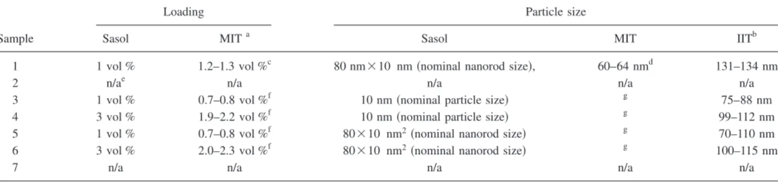
TableIIreports the information received by Sasol along with the results of some measurements done at MIT and IIT. Figure2shows transmission electron microscopy共TEM兲 im-ages for samples 1 and 3. TEM imim-ages for samples 4–6 are not available.
B. Set 2
The samples in set 2 were supplied by Dr. Lim Geok Kieng of DSO National Laboratories in Singapore. The num-bering for these samples is as follows:
共1兲 gold nanoparticles in de-ionized water and trisodium ci-trate stabilizer and
共2兲 de-ionized water+sodium citrate stabilizer 共basefluid sample兲.
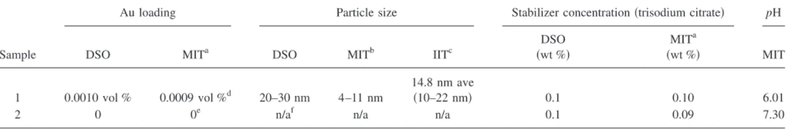
The nanofluid sample was produced according to a one-step “citrate method,” in which 100 ml of 1.18 mM gold共III兲 chloride trihydrate solution and 10 ml of 3.9 mM trisodium citrate dehydrate solution were mixed, brought to boil and stirred for 15 min. Gold nanoparticles formed as the solution was let cool to room temperature. TableIIIreports the infor-mation received by DSO National Laboratories along with the results of some measurements done at MIT and IIT. Fig-ure3 shows the TEM images for sample 1.
C. Set 3
Set 3 consisted of a single sample, supplied by W. R. Grace & Co.Silica monodispersed spherical nanoparticles and stabilizer in de-ionized water. The silica particles were synthesized by ion exchange of sodium silicate solution in a proprietary process. A general description of this process can be found in the literature.43Grace commercializes this nano-fluid as Ludox TM-50, and indicated that the nanoparticles are stabilized by making the system alkaline, the base being deprotonated silanol 共SiO−兲 groups on the surface with Na+ as the counterion共0.1–0.2 wt % of Na ions兲. The dispersion contains also 500 ppm of a proprietary biocide. Grace stated that it was not possible to supply a basefluid sample with only water and stabilizer “because of the way the particles are made.” Given the low concentration of the stabilizer and biocide, de-ionized water was assumed to be the basefluid sample, and designated “sample 2,” though it was not actu-ally sent to the participants. TableIVreports the information received by Grace along with the results of some measure-ments done at MIT. Figure4shows the TEM images for the set 3 sample.
D. Set 4
The samples in set 4 were supplied by Dr. Jorge Gustavo Gutierrez of the University of Puerto Rico-Mayaguez
TABLE II. Characteristics of the set 1 samples.
Sample
Loading Particle size
Sasol MITa Sasol MIT IITb
1 1 vol % 1.2–1.3 vol %c 80 nm⫻10 nm 共nominal nanorod size兲, 60–64 nmd 131–134 nm
2 n/ae n/a n/a n/a n/a
3 1 vol % 0.7–0.8 vol %f 10 nm共nominal particle size兲 g 75–88 nm
4 3 vol % 1.9–2.2 vol %f 10 nm共nominal particle size兲 g 99–112 nm
5 1 vol % 0.7–0.8 vol %f 80⫻10 nm2共nominal nanorod size兲 g 70–110 nm
6 3 vol % 2.0–2.3 vol %f 80⫻10 nm2共nominal nanorod size兲 g 100–115 nm
7 n/a n/a n/a n/a n/a
aRange of values is given to account for expected hydration range of alumina共boehmite兲. Boehmite’s chemical formula is Al
2O3· nH2O, where n = 1 to 2. The
hydrate is bound and cannot be dissolved in water. In most boehmites there is 70–82 wt % Al2O3per gram of powder. Boehmite density is 3.04 g/cm3. bAverage size of dispersed phase, measured by dynamic light scattering共DLS兲. The range indicates the spread of six nominally identical measurements. DLS
systemic uncertainty is of the order of⫾10 nm. Malvern NanoS used to collect data.
cMeasurements by inductive coupled plasma共ICP兲.
dAverage size of dispersed phase, measured by DLS. The range indicates the spread of multiple nominally identical measurements. DLS systemic uncertainty
is of the order of⫾10 nm.
eNot applicable.
fMeasurements by neutron activation analysis共NAA兲.
gNot available due to unreliability of DLS analyzer with PAO-based samples.
FIG. 2. Set 1—TEM pictures of samples 1共a兲 and 3 共b兲, respectively. The nanorod dimensions in sample 1 are in reasonable agreement with the nomi-nal size共80 nm⫻10 nm兲 stated by Sasol. However, smaller particles of lower aspect ratio are clearly present along with the nanorods. TEM pictures of PAO-based samples have generally been of lower quality. However, the nanoparticles in sample 3 appear to be roughly spherical and of approximate diameter 10–20 nm, thus consistent with the nominal size of 10 nm stated by Sasol.
共UPRM兲. A chemical coprecipitation method was used to synthesize the particles.44 The set 4 sample numbering is as follows:
共1兲 Mn–Zn ferrite 共Mn1/2– Zn1/2– Fe2O4兲 particles in
solu-tion of stabilizer and water and
共2兲 solution of stabilizer 共25 wt %兲 and water 共75 wt %兲 共basefluid sample兲.
The stabilizer is tetramethylammonium hydroxide or 共CH3兲4NOH. Table V reports the information received by
UPRM along with the results of some measurements done at MIT. Figure5 shows the TEM images for sample 1.
IV. THERMAL CONDUCTIVITY DATA
The thermal conductivity data generated by the partici-pating organizations are shown in Figs.6–18, one for each sample in each set. In these figures the data are anonymous, i.e., there is no correspondence between the organization number in the figures and the organization list in TableI. The data points indicate the mean value for each organization, while the error bars indicate the standard deviation calculated using the procedure described in Appendix A. The sample average, i.e., the average of all data points, is shown as a solid line, and the standard error of the mean is denoted by the dotted lines to facilitate visualization of the data spread. The standard error of the mean is typically much lower than the standard deviation because it takes into account the total
number of measurements made to arrive at the sample aver-age. Each measurement technique is denoted by a different symbol, and averages for each of the measurement tech-niques are shown. The measurement techtech-niques were grouped into four categories: the KD2 thermal properties analyzer共Decagon兲, custom thermal hot wire 共THW兲, steady state parallel plate, and other techniques. Outliers 共deter-mined using Peirce’s criterion兲 are shown as filled data points and were not included in either the technique or en-semble averages.
It can be seen that for all water-based samples in all four sets most organizations report values of the thermal conduc-tivity that are within ⫾5% of the sample average. For the PAO-based samples the spread is a little wider with most organizations reporting values that are within ⫾10% of the sample average. A note of caution is in order: while all data reported here are nominally for room temperature, what con-stitutes “room temperature” varies from organization to or-ganization. The data shown in Figs.6–18include only mea-surements conducted in the range of 20– 30 ° C. Over this range of temperatures, the thermal conductivity of the test fluids is expected to vary minimally; for example, the water thermal conductivity varies by less than 2.5%. Where de-ionized water was the basefluid共Figs.7and16兲, the range of nominal thermal conductivity of water for 20– 30 ° C is shown as a red band plotted on top of the measured data.
Figures19–26show the thermal conductivity
“enhance-TABLE III. Characteristicsf the set 2 samples.
Sample
Au loading Particle size Stabilizer concentration共trisodium citrate兲 pH
DSO MITa DSO MITb IITc
DSO 共wt %兲 MITa 共wt %兲 MIT 1 0.0010 vol % 0.0009 vol %d 20–30 nm 4–11 nm 14.8 nm ave 共10–22 nm兲 0.1 0.10 6.01
2 0 0e n/af n/a n/a 0.1 0.09 7.30
aMeasurements by inductive coupled plasma共ICP兲. ICP has an accuracy of 0.6% of the reported value for gold in the concentration range of interest. bNumber-weighted average size of particles, measured by DLS. The range indicates the spread of two nominally identical measurements. DLS systemic
uncertainty is of the order of⫾10 nm.
cMeasurements by DLS. The values reported are the number-weighted average and the range at the full-width half maximum for six measurements. dAssumed density of gold is 19.32 g/cm3.
eWithin the detection limit of ICP. fNot applicable.
FIG. 3. Set 2—TEM pictures of sample 1. The nanoparticles are roughly spherical and of diameter⬍20 nm, thus somewhat smaller than the nominal size of 20–30 nm stated by DSO National Laboratories.
FIG. 4. Set 3—TEM pictures of sample 1. The nanoparticles are roughly spherical and of diameter 20–30 nm, thus consistent with the nominal size of 22 nm stated by Grace.
TABLE IV. Characteristics of the set 3 samples.
Sample
Silica共SiO2兲 loading Na2SO4concentration Particle size pH
Grace MIT Grace MITa Grace MITb Grace MIT
1 49.8 wt % 43.6 wt %a 0.1–0.2 wt % of Na 0.27 wt % of Na 22 nm 20–40 nm 8.9 9.03 31.1 vol %c 26.0 vol %c
2d n/ae n/a n/a n/a n/a n/a n/a n/a
aMeasured by inductive coupled plasma共ICP兲. ICP has an accuracy of 0.6% of the reported value.
bNumber-weighted average size of particles, measured by dynamic light scattering 共DLS兲. The range indicates the spread of three nominally identical
measurements. DLS systemic uncertainty is of the order of⫾10 nm.
cAssumed density of silica共SiO
2兲 is 2.2 g/cm3.
dSample 2 is simply de-ionized water, which was assumed to be the basefluid sample, but was not actually sent to the participants. eNot applicable.
TABLE V. Characteristics of the set 4 samples.
Sample
Particle loading Particle composition Particle size pH
UPRM MIT UPRM MITa UPRM MIT MIT
1 0.17 vol %b 0.16 vol %c Mn1/2– Zn1/2– Fe2d Mn⬃15 at. %, 7.4 nme 6–11 nmf 15.2
Zn⬃14 at. %, Fe⬃71 at. %
2 n/ag n/a n/a n/a n/a n/a 15.1
aAtomic fraction of metals measured by energy dispersive x-ray spectroscopy共EDS兲. bDetermined from magnetic measurements.
cMeasurements by inductive coupled plasma共ICP兲. Assumed density of 4.8 g/cm3for Mn–Zn ferrite. ICP has an accuracy of 0.6% of the reported value. dThe molar fraction of Mn and Zn was determined from stoichiometric balance.
eAverage magnetic particle diameter.
fNumber-weighted average size of particles, measured by dynamic light scattering 共DLS兲. The range indicates the spread of four nominally identical
measurements. DLS systemic uncertainty is of the order of⫾10 nm.
gNot applicable.
FIG. 5. Set 4—TEM pictures of sample 1. The nanoparticles have irregular shape and approximate size⬍20 nm, thus consistent with the nominal size of⬃7 nm stated by UPRM.
FIG. 6.共Color兲 Thermal conductivity data for sample 1, set 1.
FIG. 7. 共Color兲 Thermal conductivity data for sample 2 共basefluid兲, set 1.
FIG. 9.共Color兲 Thermal conductivity data for sample 4, set 1.
FIG. 10.共Color兲 Thermal conductivity data for sample 5, set 1.
FIG. 11.共Color兲 Thermal conductivity data for sample 6, set 1.
FIG. 12.共Color兲 Thermal conductivity data for sample 7, set 1.
FIG. 13.共Color兲 Thermal conductivity data for sample 1, set 2.
FIG. 14.共Color兲 Thermal conductivity data for sample 2, set 2.
FIG. 15.共Color兲 Thermal conductivity data for sample 1, set 3.
FIG. 16. 共Color兲 Thermal conductivity data for sample 2 共basefluid兲, set 3.
FIG. 17.共Color兲 Thermal conductivity data for sample 1, set 4.
FIG. 19. 共Color兲 Thermal conductivity enhancement data for sample 1, set 1.
FIG. 20. 共Color兲 Thermal conductivity enhancement data for sample 3, set 1.
FIG. 21. 共Color兲 Thermal conductivity enhancement data for sample 4, set 1.
FIG. 22. 共Color兲 Thermal conductivity enhancement data for sample 5, set 1.
FIG. 23. 共Color兲 Thermal conductivity enhancement data for sample 6, set 1.
FIG. 24. 共Color兲 Thermal conductivity enhancement data for sample 1, set 2.
FIG. 25. 共Color兲 Thermal conductivity enhancement data for sample 1, set 3.
FIG. 26. 共Color兲 Thermal conductivity enhancement data for sample 1, set 4.
ment” for all nanofluid samples, i.e., the ratio of the nano-fluid thermal conductivity to the basenano-fluid thermal conduc-tivity. For each organization, the data point represents the ratio of the mean thermal conductivities of the nanofluid and basefluid, while the error bars represent the standard devia-tion calculated according to the procedure described in Ap-pendix A. If a participating organization did not measure the basefluid thermal conductivity in their laboratory, a calcula-tion of enhancement was not made. Again, the sample aver-age is shown as a solid line along with the standard error of the mean, and outliers are indicated by filled data points. Note that there is reasonable consistency 共within ⫾5%兲 in the thermal conductivity ratio data among most organizations and for all four sets, including water-based and PAO-based samples.
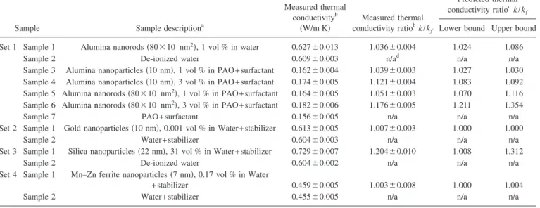
The INPBE database is summarized in TableVI. Com-paring the data for samples 3, 4, 5, and 6 in set 1, it is noted that, everything else being the same, the thermal conductiv-ity enhancement is higher at higher particle concentration, and higher for elongated particles than for near-spherical par-ticles. Comparing the data for samples 1 and 5 in set 1, it is noted that the thermal conductivity enhancement is some-what higher for the PAO basefluid than for water. The set 2 data suggest that the thermal conductivity enhancement is negligible, if the particle concentration is very low, even if metal particles of high thermal conductivity are used. On the other hand, the set 3 data suggest that a robust enhancement can be achieved, if the particle concentration is high, even if the particle material has a modest thermal conductivity. All these trends are expected, based on the effective medium theory, as will be discussed in Sec. V below.
A. Effects of the experimental approach on the thermal conductivity measurements
TableIreports the experimental techniques used by the various organizations to measure thermal conductivity, and
provides, when available, a reference where more informa-tion about those techniques can be found. Transient, steady-state, and optical techniques were used to measure thermal conductivity. There are transient measurement techniques that require the immersion of a dual heating and sensing element in the sample, such as the transient hot wire共THW兲 and transient hot disk techniques. The THW technique is based on the relationship between the thermal response of a very small 共⬍100 m兲 diameter wire immersed in a fluid sample to a step change in heating and the thermal conduc-tivity of the fluid sample.45The THW technique was used by over half of the participating organizations, many of which used a custom built apparatus. The KD2 thermal properties analyzer made by Decagon, an off-the-shelf device that is based on the THW approach, was also used. The transient hot disk technique is similar to the THW technique, except that the heater/sensor is a planar disk coated in Kapton.46In steady-state techniques such as the parallel plate47 and co-axial cylinder48 methods, heat is transferred between two plates共or coaxial cylinders兲 sandwiching the test fluid. Mea-surement of the temperature difference and heat transfer rate across the fluid can be used to determine the thermal con-ductivity via Fourier’s law. The thermal comparator method, also a steady-state method, measures the voltage difference between a heated probe in point contact with the surface of the fluid sample and a reference, which can be converted to thermal conductivity using a calibration curve of samples of known conductivity.49 In the forced Rayleigh scattering method, an optical grating is created in a sample of the fluid using the intersection of two beams from a high-powered laser. The resulting temperature change causes small-scale density changes that create a refraction index grating that can be detected using another laser. The relaxation time of the refraction index grating is related to the thermal diffusivity of the fluid from which the thermal conductivity can be evaluated.50
TABLE VI. Summary of INPBE results.
Sample Sample descriptiona
Measured thermal conductivityb 共W/m K兲 Measured thermal conductivity ratiobk/kf Predicted thermal conductivity ratiock/kf
Lower bound Upper bound
Set 1 Sample 1 Alumina nanorods共80⫻10 nm2兲, 1 vol % in water 0.627⫾0.013 1.036⫾0.004 1.024 1.086
Sample 2 De-ionized water 0.609⫾0.003 n/ad n/a n/a
Sample 3 Alumina nanoparticles共10 nm兲, 1 vol % in PAO+surfactant 0.162⫾0.004 1.039⫾0.003 1.027 1.030 Sample 4 Alumina nanoparticles共10 nm兲, 3 vol % in PAO+surfactant 0.174⫾0.005 1.121⫾0.004 1.083 1.092 Sample 5 Alumina nanorods共80⫻10 nm2兲, 1 vol % in PAO+surfactant 0.164⫾0.005 1.051⫾0.003 1.070 1.116
Sample 6 Alumina nanorods共80⫻10 nm2兲, 3 vol % in PAO+surfactant 0.182⫾0.006 1.176⫾0.005 1.211 1.354
Sample 7 PAO+ surfactant 0.156⫾0.005 n/a n/a n/a
Set 2 Sample 1 Gold nanoparticles共10 nm兲, 0.001 vol % in Water+stabilizer 0.613⫾0.005 1.007⫾0.003 1.000 1.000
Sample 2 Water+ stabilizer 0.604⫾0.003 n/a n/a n/a
Set 3 Sample 1 Silica nanoparticles共22 nm兲, 31 vol % in Water+stabilizer 0.729⫾0.007 1.204⫾0.010 1.008 1.312
Sample 2 De-ionized water 0.604⫾0.002 n/a n/a n/a
Set 4 Sample 1 Mn–Zn ferrite nanoparticles共7 nm兲, 0.17 vol % in Water
+ stabilizer 0.459⫾0.005 1.003⫾0.008 1.000 1.004
Sample 2 Water+ stabilizer 0.455⫾0.005 n/a n/a n/a
aNominal values for nanoparticle concentration and size. bSample average and standard error of the mean. cCalculated with the assumptions in Appendix B. dNot applicable.
The measurement techniques were grouped into KD2, custom THW, parallel plate, and other共which include ther-mal comparator, hot disk, forced Rayleigh scattering, and coaxial cylinders兲. Thermal conductivity and enhancement data for each group of measurement techniques is shown in Figs.6–26.
For each of the four measurement technique groupings, the average thermal conductivity is shown on the plot and is indicated by the solid line. In the custom THW data on Figs. 6 and 7, there is one measurement that is well above the average in both figures. This was the only THW apparatus with an uninsulated wire. Typically an insulated wire is used in this method to reduce the current leakage into the fluid. The higher thermal conductivity measured here may be a result of that effect. Excepting the outliers, all the measure-ment techniques show good agreemeasure-ment for de-ionized water 共Figs.7 and16兲. For the PAO basefluid 共Fig.12兲 the unin-sulated hot wire measurement共organization 14兲 is no longer an outlier. PAO is not as electrically conductive as water, and the current leakage effect should be less of an issue for this fluid.
As described in Appendix A, a fixed effects model was used to determine whether differences in the data from dif-ferent measurement techniques are statistically significant. Because of the low number of data points in the parallel plate and Other categories, only the KD2 and custom hot wire techniques were compared. For all the samples in sets 1, 2, and 3, the KD2 thermal conductivity average is lower than the custom THW average. The fixed effects model shows that this is a statistically significant difference for samples 1, 3, 4, 6, and 7, in set 1, and sample 2 in set 3. In set 4, the KD2 average is higher than the Custom THW, but this dif-ference is statistically significant only for sample 2 共the water+ stabilizer basefluid for the ferrofluid兲. It is not clear why the KD2 measurements are lower than the THW mea-surements for all fluids except those in set 4. Finally, in most cases, there is less scatter in the KD2 data for the PAO-based nanofluids than the water-based nanofluids. This may be due to the higher viscosity of the PAO, which counteracts ther-mal convection during the 30 s KD2 heating cycle.
It is difficult to make specific conclusions about thermal conductivity measurements using the parallel plate technique due to the low number of data points and the amount of scatter for some samples共see Figs.13–15兲. Additional mea-surements would be needed to determine if there is a system-atic difference between the parallel plate technique and other techniques.
Although the thermal conductivity data show some clear differences in measurement technique, these differences be-come less apparent once the data are normalized with the basefluid thermal conductivities共Figs.19–26兲. A comparison of the KD2 and THW techniques was again performed using the fixed effects model. The only statistically significant dif-ference between the two techniques was for set 1, sample 4 共Fig.21兲, the 3% volume fraction alumina-PAO nanofluid.
This study shows that the choice of measurement tech-nique can affect the measured value of thermal conductivity, but if the enhancement is the parameter of interest, the mea-surement technique is less important, at least for the KD2
and THW techniques. Therefore, to ensure accurate determi-nations of nanofluid thermal conductivity enhancement using these techniques, it is important to measure both the base-fluid and nanobase-fluid thermal conductivity using the same tech-nique and at the same temperature.
V. COMPARISON OF DATA TO EFFECTIVE MEDIUM THEORY
Equation 共1兲 is valid for well-dispersed noninteracting spherical particles with negligible thermal resistance at the particle/fluid interface. To include the effects of particle ge-ometry and finite interfacial resistance, Nan et al.51 general-ized Maxwell’s model to yield the following expression for the thermal conductivity ratio:
k kf
=3 +关211共1 − L11兲 +33共1 − L33兲兴 3 −共211L11+33L33兲
, 共2兲
where for particles shaped as prolate ellipsoids with principal axes a11= a22⬍a33 L11= p2 2共p2− 1兲− p 2共p2− 1兲3/2cosh−1p, L33= 1 − 2L11, p = a33/a11, ii= kii c − kf kf+ Lii共kii c − kf兲 , kii c = kp 1 +␥Liikp/kf , ␥=共2 + 1/p兲Rbdkf/共a11/2兲,
and Rbd is the 共Kapitza兲 interfacial thermal resistance. The
limiting case of very long aspect ratio in the theory of Nan et
al. is bounded by the nanoparticle linear aggregation models
proposed by Prasher et al.37, Keblinski et al.52, and Eapen.53 Obviously, Eq.共2兲 reduces to Eq. 共1兲 for spherical particles 共p=1兲 and negligible interfacial thermal resistance 共Rbd= 0兲,
as it can be easily verified. Equation 共2兲 predicts that, if kp
⬎kf, the thermal conductivity enhancement increases with
increasing particle loading, increasing particle aspect ratio and decreasing basefluid thermal conductivity, as observed for the data in INPBE set 1. More quantitatively, the theory was applied to the INPBE test nanofluids with the assump-tions reported in Appendix B. Figure27shows the
cumula-FIG. 27. 共Color兲 Percentage of all INPBE experimental data that are pre-dicted by the theory of Nan et al. within the error indicated on the x-axis.
tive accuracy information of the effective medium theory for all the INPBE data. Two curves are shown: one for zero interfacial thermal resistance 共upper bound兲, and one for a typical value of the interfacial resistance, 10−8 m2K/W.54–56
It can be seen that all INPBE data can be predicted by the lower bound theory with⬍17% error, while the upper bound estimate predicts 90% of the data with ⬍18% error.
The above data analysis demonstrates that our colloi-dally stable nanofluids exhibit thermal conductivity in good agreement with the predictions of the effective medium theory for well-dispersed nanoparticles. That is, no anoma-lous thermal conductivity enhancement was observed for the nanofluids tested in this study. As such, resorting to the other theories proposed in the literature 共e.g., Brownian motion, liquid layering, and aggregation兲 is not necessary for the in-terpretation of the INPBE database. It should be noted, how-ever, that the ranges of parameters explored in INPBE, while broad, are not exhaustive. For example, only one nanofluid with metallic nanoparticles was tested, and only at very low concentration. Also, the temperature effect on thermal con-ductivity was not investigated.
VI. CONCLUSIONS
An international nanofluid property benchmark exercise, or INPBE, was conducted by 34 organizations participating from around the world. The objective was to compare ther-mal conductivity data obtained by different experimental ap-proaches for identical samples of various nanofluids. The main findings of the study were as follows.
共1兲 The thermal conductivity enhancement afforded by the tested nanofluids increased with increasing particle load-ing, particle aspect ratio and decreasing basefluid ther-mal conductivity.
共2兲 For all water-based samples tested, the data from most organizations deviated from the sample average by⫾5% or less. For all PAO-based samples tested, the data from most organizations deviated from the sample average by ⫾10% or less.
共3兲 The classic effective medium theory for well-dispersed particles accurately reproduced the INPBE experimental data; thus, suggesting that no anomalous enhancement of thermal conductivity was observed in the limited set of nanofluids tested in this exercise.
共4兲 Some systematic differences in thermal conductivity measurements were seen for different measurement techniques. However, as long as the same measurement technique at the same temperature conditions was used to measure the thermal conductivity of the basefluid, the thermal conductivity enhancement was consistent be-tween measurement techniques.
ACKNOWLEDGMENTS
This work was made possible by the support of the Na-tional Science Foundation under Grant No. CBET-0812804. The authors are also grateful to Sasol and W. R. Grace & Co. for donating some of the samples used in INPBE. Special
thanks to Mr. Edmund Carlevale of MIT for creating and maintaining the INPBE website.
APPENDIX A: STATISTICAL TREATMENT OF DATA
For each fluid sample, the thermal conductivity raw data 共xi1, xi2, . . . , xini兲 from the ith organization were processed to
estimate the organization’s mean共x¯i兲 and standard deviation
共si兲, respectively, as x ¯i= 1 ni
兺
j=1 ni xij and si=冑
1 ni− 1兺
j=1 ni 共xij− x¯i兲2. 共A1兲The values of x¯i and si for each organization are shown in
Figs. 6–18 as data points and error bars, respectively. The normality of the xijdata sets was checked using the Shapiro–
Francia W
⬘
test57 and was found to be satisfactory. Peirce’s criterion58 was used to identify outliers which were not in-cluded in the sample average and variance calculations de-scribed below, but are shown in Figs. 6–18 as filled data points.The analysis of data among different organizations was carried out using the random effects model.57In the random effects model, an assumption is made that the conclusions from the analysis can be applied to a wider class of measure-ments of which the ni populations共or organizations, in this
case兲 are a representative subset. The model assumes that
xij=+␣i+ eij, 共A2兲
where is the estimator of the sample mean,␣i is the
sys-tematic error for each organization共which are treated as ran-dom errors among organizations兲, and eij is the random or
unexplained error for each measurement. It is helpful to note that
␣i= x¯i−,
eij= xij− x¯i. 共A3兲
It is assumed that ␣i and eij are normally distributed with
zero means and standard deviations of a and e,
respec-tively. The normality of the eijdata sets was checked using
the Shapiro–Francia W
⬘
test and was found to be satisfactory. This analysis assumes that standard deviations within the organizations are equal 共i=e兲. This was checked byper-forming pair-wise F-tests on i.
The standard random effects model uses a weighted av-erage as the sample avav-erage共taking into account the number of data points reported by each organization兲,
= x¯ = 1 N
兺
i=1I
ni¯xi. 共A4兲
We believe that this definition overemphasizes the contribu-tions from organizacontribu-tions that reported many data points. For the purposes of this study, a more appropriate estimator of the sample mean is an unweighted average of organization averages given in the following equation:
x ¯ =1 I
兺
i=1 I x ¯i. 共A5兲This way, each organization contributes equally to the en-semble average. This estimator has been analyzed in the literature57 and its variance is given by
2= Var共x¯兲 = 1 I2
兺
i=1 I冉
e 2 ni +a 2冊
, 共A6兲 where e2= 1 共N − I兲兺
i=1 I 共ni− 1兲si2, 共A7兲 N =兺
i=1 I ni, 共A8兲 a 2 =共MSA −e 2兲 no , 共A9兲 MSA = 1 共I − 1兲冉
兺
i=1 I ni¯xi 2 − Nx¯2冊
, 共A10兲 no= 1 I − 1冢
N − 兺 i=1 I ni2 N冣
. 共A11兲The standard error共兲 of the unweighted average is shown in Figs. 6–18 as dotted lines plotted above and below the sample average. The literature shows that the estimator共A5兲 is preferred over the estimator共A4兲 ifa2⬎e2.
57,59
The sta-tistical analysis shows that this condition is satisfied for the INPBE data.
Thermal conductivity enhancements were determined from the ratio of the nanofluid thermal conductivity to the basefluid thermal conductivity and are given as yi. If an
or-ganizational mean for a given fluid sample was identified as an outlier in the thermal conductivity analysis, it was not excluded here in determining enhancements. A second round of applying the Peirce criterion excluded those enhancements that were outliers.
The standard deviation 共error bars兲 of the thermal con-ductivity enhancements共data points兲 for individual organiza-tions shown in Figs. 19–26were calculated by propagating the standard deviation of the numerator and denominator.60 That is, if y = xnf/xbf, then:
senh y =
冑
冉
snf xnf冊
+冉
sbf xbf冊
. 共A12兲The procedure for calculating the thermal conductivity en-hancement sample average and its variance was based on Eqs. 共A5兲–共A11兲, where the thermal conductivity for each organization, x¯i, is replaced by the thermal conductivity
en-hancement for each organization, y¯i, and ni is the harmonic
average of the total number of measurements used to calcu-late the enhancement.
To compare the different measurement techniques, the fixed effects model was used.57For each technique, the tech-nique average and the variance were determined using Eqs. 共A5兲–共A11兲above. For an unbalanced data set共one in which there are a different number of data points for each measure-ment technique to be compared兲, the approximate Tukey– Kramer intervals were used, which depend on the probability statement, P
再
i−i⬘苸 y¯i− y¯i⬘⫾ q␣,k,si冋
1 2冉
1 ni + 1 ni⬘冊
册
1/2for all i,i
⬘
冎
= 1 −␣, 共A13兲 where q␣,k, is the upper␣ point of the “studentized” range distribution for k 共the number of measurement techniques compared兲 and , the degrees of freedom 共N−k兲. If the in-terval given in Eq.共A12兲does not contain zero for any com-bination of two measurement techniques, then the difference in technique mean is statistically significant.APPENDIX B: ASSUMPTIONS USED IN THE EFFECTIVE MEDIUM MODEL FOR THERMAL CONDUCTIVITY
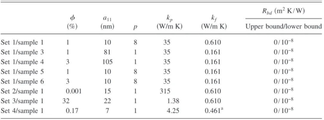
Use of the model of Nan et al. requires input of the values of the particle volumetric fraction共兲, particle mini-mum axis 共a11兲, particle aspect ratio 共p兲, particle thermal
conductivity 共kp兲, basefluid thermal conductivity 共kf兲, and TABLE VII. Input for effective medium model calculations.
共%兲 a11 共nm兲 p kp 共W/m K兲 kf 共W/m K兲 Rbd共m2K/W兲
Upper bound/lower bound
Set 1/sample 1 1 10 8 35 0.610 0/10−8 Set 1/sample 3 1 81 1 35 0.161 0/10−8 Set 1/sample 4 3 105 1 35 0.161 0/10−8 Set 1/sample 5 1 10 8 35 0.161 0/10−8 Set 1/sample 6 3 10 8 35 0.161 0/10−8 Set 2/sample 1 0.001 15 1 315 0.610 0/10−8 Set 3/sample 1 32 22 1 1.38 0.610 0/10−8 Set 4/sample 1 0.17 7 1 4.25 0.461a 0/10−8
interfacial thermal resistance共Rbd兲. The nominal values used
to generate the curves in Fig.27are shown in TableVII.
1J. A. Eastman, S. R. Phillpot, S. U. S. Choi, and P. Keblinski,Annu. Rev.
Mater. Res.34, 219共2004兲.
2S. K. Das, S. U. S. Choi, and H. E. Patel,Heat Transfer Eng.27, 3共2006兲. 3S. Kabelac and J. F. Kuhnke, Annals of the Assembly for International
Heat Transfer Conference, 2006共unpublished兲, Vol. 13, p. KN-11.
4V. Trisaksri and S. Wongwises,Renewable Sustainable Energy Rev.11,
512共2007兲.
5X. Q. Wang and A. S. Mujumdar,Int. J. Therm. Sci.46, 1共2007兲. 6S. M. S. Murshed, K. C. Leong, and C. Yang,Appl. Therm. Eng.28, 2109
共2008兲.
7W. Yu, D. M. France, J. L. Routbort, and S. U. S. Choi,Heat Transfer Eng. 29, 432共2008兲.
8S. K. Das, S. U. S. Choi, W. Yu, and T. Pradeep, Nanofluids: Science and
Technology共Wiley, New York, 2008兲.
9J. C. Maxwell, A Treatise on Electricity and Magnetism, 2nd ed.
共Claren-don, Oxford, 1881兲.
10Q. Li and Y. M. Xuan, in Heat Transfer Science and Technology, edited by
B. Wang共Higher Education Press, Beijing, 2000兲, pp. 757–762.
11J. A. Eastman, S. U. S. Choi, S. Li, W. Yu, and L. J. Thompson,Appl.
Phys. Lett.78, 718共2001兲.
12H. U. Kang, S. H. Kim, and J. M. Oh,Exp. Heat Transfer19, 181共2006兲. 13T.-K. Hong, H. Yang, and C. J. Choi,J. Appl. Phys.97, 064311共2005兲. 14S. Jana, A. Salehi-Khojin, and W. H. Zhong,Thermochim. Acta462, 45
共2007兲.
15M. Chopkar, P. K. Das, and I. Manna,Scr. Mater.55, 549共2006兲. 16S. Shaikh, K. Lafdi, and R. Ponnappan,J. Appl. Phys.101, 064302共2007兲. 17H. Xie, J. Wang, T. Xi, and F. Ai,J. Appl. Phys.91, 4568共2002兲. 18H. Xie, J. Wang, T. Xi, and Y. Liu,Int. J. Thermophys.23, 571共2002兲. 19S. M. S. Murshed, K. C. Leong, and C. Yang,Int. J. Therm. Sci.44, 367
共2005兲.
20C. H. Chon, K. D. Kihm, S. P. Lee, and S. U. S. Choi,Appl. Phys. Lett. 87, 153107共2005兲.
21K. S. Hong, T.-K. Hong, and H.-S. Yang,Appl. Phys. Lett.88, 031901
共2006兲.
22S. H. Kim, S. R. Choi, and D. Kim, ASME J. Heat Transfer129, 298
共2007兲.
23C. H. Li and G. P. Peterson,J. Appl. Phys.101, 044312共2007兲. 24G. Chen, W. H. Yu, D. Singh, D. Cookson, and J. Routbort,J. Nanopart.
Res.10, 1109共2008兲.
25P. D. Shima, J. Philip, and B. Raj, Appl. Phys. Lett. 94, 223101共2009兲. 26S. K. Das, N. Putra, P. Thiesen, and W. Roetzel,ASME J. Heat Transfer
125, 567共2003兲.
27D. Wen and Y. Ding,J. Thermophys. Heat Transfer18, 481共2004兲. 28C. H. Li and G. P. Peterson,J. Appl. Phys.99, 084314共2006兲. 29H. D. Kumar, H. E. Patel, K. V. R. Rajeev, T. Sundararajan, T. Pradeep,
and S. K. Das,Phys. Rev. Lett.93, 144301共2004兲.
30S. P. Jang and S. U. S. Choi,Appl. Phys. Lett.84, 4316共2004兲. 31R. Prasher, P. Bhattacharya, and P. E. Phelan,Phys. Rev. Lett.94, 025901
共2005兲.
32H. E. Patel, T. Sundararajan, T. Pradeep, A. Dasgupta, N. Dasgupta, and S.
K. Das,Pramana, J. Phys.65, 863共2005兲.
33H. E. Patel, T. Sundararajan, and S. K. Das,J. Nanopart. Res. 10, 87
共2008兲.
34P. Keblinski, S. R. Phillpot, S. U. S. Choi, and J. A. Eastman,Int. J. Heat
Mass Transfer45, 855共2002兲.
35B. X. Wang, L. P. Zhou, and X. F. Peng,Int. J. Heat Mass Transfer46,
2665共2003兲.
36M. Foygel, R. D. Morris, D. Anez, S. French, and V. L. Sobolev,Phys.
Rev. B71, 104201共2005兲.
37R. Prasher, W. Evans, P. Meakin, J. Fish, P. Phelan, and P. Keblinski,
Appl. Phys. Lett.89, 143119共2006兲.
38J. Eapen, J. Li, and S. Yip,Phys. Rev. E76, 062501共2007兲.
39J. Philip, P. D. Shima and R. Baldev,Nanotechnology19, 305706共2008兲. 40W. Yu and S. U. S. Choi,J. Nanopart. Res.5, 167共2003兲.
41J. Eapen, J. Li, and S. Yip,Phys. Rev. Lett.98, 028302共2007兲.
42J. Eapen, W. C. Williams, J. Buongiorno, L. W. Hu, S. Yip, R. Rusconi,
and R. Piazza,Phys. Rev. Lett.99, 095901共2007兲.
43R. K. Iler, The Chemistry of Silica共Wiley, New York, 1979兲, Chap. 4. 44J. G. Gutierrez and M. Riccetti, Proceedings of the ASME International
Mechanical Engineering Congress and Exposition, Boston, Massachusetts, 31 October–6 November 2008共unpublished兲.
45J. J. Healy, J. J. de Groot, and J. Kestin,Physica C82, 392共1976兲. 46T. Boumaza and J. Redgrove,Int. J. Thermophys.24, 501共2003兲. 47R. G. Miller and L. S. Fletcher, Proceedings of the Tenth Southeastern
Seminar on Thermal Sciences, New Orleans, LA, 1974共unpublished兲, pp. 263–285.
48H. Ziebland, in Thermal Conductivity, edited by R. P. Tye 共Academic,
London, 1969兲, Vol. 2, pp. 96–110.
49R. W. Powell, in Thermal Conductivity, edited by R. P. Tye共Academic,
London, 1969兲, Vol. 2, pp. 288–295.
50H. Eichler, G. Salje, and H. Stahl,J. Appl. Phys.44, 5383共1973兲. 51C. W. Nan, R. Birringer, D. R. Clarke, and H. Gleiter,J. Appl. Phys.81,
6692共1997兲.
52P. Keblinski, R. Prasher, and J. Eapen,J. Nanopart. Res.10, 1089共2008兲. 53J. Eapen, Thermal conduction mechanism in nanofluids, solid composites
and liquid mixtures, Proceedings of 2009 ASME Summer Heat Transfer
Conference共HT2009-88236兲, July 19-23, 2009, San Francisco, CA.
54O. M. Wilson, X. Hu, D. G. Cahill, and P. V. Braun,Phys. Rev. B66,
224301共2002兲.
55S. Huxtable, D. G. Cahill, S. Shenogin, L. Xue, R. Ozisik, P. Barone, M.
Usrey, M. S. Strano, G. Siddons, M. Shim, and P. Keblinski,Nature Mater. 2, 731共2003兲.
56E. V. Timofeeva, A. N. Gavrilov, J. M. McCloskey, Y. V. Tolmachev, S.
Sprunt, L. M. Lopatina, and J. V. Selinger, Phys. Rev. E 76, 061203
共2007兲.
57R. G. Miller, Beyond ANOVA, Basics of Applied Statistics共CRC, Boca
Raton, 1997兲, pp. 69–111.
58S. M. Ross, J. Engineering Technology 20, 38共2003兲.
59G. W. Snedecore and W. G. Cochran, Statistical Methods 共Iowa State
University Press, Ames, 1989兲.
60H. Motulsky, Intuitive Biostatistics共Oxford University Press, New York,
1995兲, pp. 284–286.
61J. Glory, M. Bonetti, M. Helezen, M. Mayne-L’Hermite, and C. Reynaud,
J. Appl. Phys.103, 094309共2008兲.
62N. Shalkevich, W. Escher, T. Buergi, B. Michel, L. Si-Ahmed, and D.
Poulikakos, “On the thermal conductivity of gold nanoparticle colloids,” Langmuir共in press兲.
63D. C. Venerus, M. S. Kabahdi, S. Lee, and V. Perez-Luna,J. Appl. Phys. 100, 094310共2006兲.
64J.-H. Lee, K. S. Hwang, S. P. Jang, B. H. Lee, J. H. Kim, S. U. S. Choi,
and C. J. Choi,Int. J. Heat Mass Transfer51, 2651共2008兲.
65R. Rusconi, W. C. Williams, J. Buongiorno, R. Piazza, and L. W. Hu,Int.
J. Thermophys.28, 1131共2007兲.
66J. Garg, B. Poudel, M. Chiesa, J. B. Gordon, J. J. Ma, J. B. Wang, Z. F.
Ren, Y. T. Kang, H. Ohtani, J. Nanda, G. H. McKinley, and G. Chen,J.
Appl. Phys.103, 074301共2008兲.
67J. Townsend and R. Christianson, Proceedings of the 17th Symposium on
Thermophysical Properties, Boulder, CO, 21–16 June 2009共unpublished兲.
68A. Jarzebski, M. Palica, A. Gierczycki, K. Chmiel-Kurowska, and G.
Dzido, Silesian University of Technology Internal Report No. BW-459/ RCh6/2007/6, 2007.
69B. Wright, D. Thomas, H. Hong, L. Groven, J. Puszynski, D. Edward, X.
Ye, and S. Jin,Appl. Phys. Lett.91, 173116共2007兲.
70P. E. Gharagozloo and K. E. Goodson, Appl. Phys. Lett. 93, 103110
共2008兲.
71S. Van Vaerenbergh, T. Maré, C. Tam Nguyen, and A. Guerin, VIII-ème
Colloque Interuniversitaire Franco-Québécois sur la Thermique des Systèmes, Montréal, Canada, 28–30 May 2007共unpublished兲.
72D. Wen and Y. Ding,IEEE Trans. Nanotechnol.5, 220共2006兲. 73J. G. Gutierrez and R. Rodriguez, Proceedings of the ASME International
Mechanical Engineering Congress and Exposition, Seattle, Washington, 11–15 November 2007共unpublished兲.