Dynamic programming applied to electromagnetic satellite actuation

(1)

Dynamic Programming Applied to

Electromagnetic Satellite Actuation

by

Gregory John Eslinger

B.S., United States Air Force Academy (2011)

Submitted to the Department of Aeronautics and Astronautics

in partial fulfillment of the requirements for the degree of

Master of Science in Aeronautics and Astronautics

at the

MASSACHUSETTS INSTITUTE OF TECHNOLOGY

June 2013

This material is declared a work of the U.S. Government and is not

subject to copyright protection in the United States

Author . . . .

Department of Aeronautics and Astronautics

May 22, 2013

Certified by. . . .

Alvar Saenz-Otero

Principal Research Scientist

Thesis Supervisor

Certified by. . . .

David W. Miller

Professor of Aeronautics and Astronautics

Thesis Supervisor

Accepted by . . . .

Eytan H. Modiano

Professor of Aeronautics and Astronautics

Chair, Graduate Program Committee

(2)

Disclaimer: The views expressed in this thesis are those of the author and do not reflect the official policy or position of the United States Air Force, Department of

(3)

Dynamic Programming Applied to Electromagnetic Satellite

Actuation

by

Gregory John Eslinger

Submitted to the Department of Aeronautics and Astronautics on May 22, 2013, in partial fulfillment of the

requirements for the degree of

Master of Science in Aeronautics and Astronautics

Abstract

Electromagnetic formation flight (EMFF) is an enabling technology for a number of space mission architectures. While much work has been done for EMFF control for large separation distances, little work has been done for close-proximity EMFF control, where the system dynamics are quite complex. Dynamic programming has been heavily used in the optimization world, but not on embedded systems. In this thesis, dynamic programming is applied to satellite control, using close-proximity EMFF control as a case study. The concepts of dynamic programming and approx-imate dynamic programming are discussed. Several versions of the close-proximity EMFF control problem are formulated as a dynamic programming problems. One of the formulations is used as a case study for developing and examining the cost-to-go. Methods for implementing an approximate dynamic programming controller on a satellite are discussed. Methods for resolving physical states and dynamic program-ming states are presented. Because the success of dynamic programprogram-ming depends on the system model, a novel method for finding the mass properties of a satellite, which would likely be used in the dynamic programming model, is introduced. This method is used to characterize the mass properties of three satellite systems: SPHERES, VERTIGO, and RINGS. Finally, a method for position and attitude estimation for systems that use line-of-sight measurements that does not require the use of a model is developed. This method is useful for model validation of the models used in the dynamic programming formulation.

Thesis Supervisor: Alvar Saenz-Otero Title: Principal Research Scientist

Thesis Supervisor: David W. Miller

(4)

(5)

Acknowledgments

I would like to thank the Air Force for allowing me the opportunity to attend graduate school. I would also like to recognize a number of people and entities for their support of RINGS.

• DARPA, especially Dave Barnhart.

• Aurora Flight Sciences, including John, Roedolph, and Joanne.

• The RINGS team at the University of Maryland: Allison Porter, Dustin Alinger, and Dr. Raymond Sedwick.

• My thesis supervisors, Prof. Miller and Dr. Saenz-Otero. I would also like to recognize the following people:

• Alex Buck, my partner in crime. Despite you being in the Navy, we managed to make a good team. Best of luck.

• Bruno Alvisio, good luck carrying on RINGS.

• Hal Schmidt and Evan Wise, its been a pleasure working at the mill with you gentlemen. May our adventures in California prove even more fruitful.

• My fellow labmates and SPHERES team members. Keep up the good work. • Michael Frossard, for keeping America safe (or at least training to) while I wrote

this work.

(6)

(7)

List of Figures

1-1 Scope of Motivation . . . 17

1-2 Example of a Mission Architecture That Uses Wireless Power Transfer 23 1-3 Example of Non-Keplerian Orbits Using EMFF . . . 24

1-4 RINGS and SPHERES During an RGA Flight . . . 25

1-5 Linear Track EMFF Testbed . . . 29

1-6 3 DoF EMFF Testbed . . . 30

1-7 µEMFF Testbed . . . 30

2-1 Simple Markov Process . . . 35

2-2 Dynamic Programming Analysis of a Simple Markov Process . . . 36

2-3 Stochastic Shortest Path Markov Process . . . 41

2-4 Illustration of State Aggregation . . . 43

2-5 Aggregation Formulation . . . 44

2-6 Illustration of Aggregation Techniques . . . 44

2-7 Controller Development Using Dynamic Programming . . . 49

3-1 Definition of Two Coils in Proximity . . . 52

3-2 General RINGS State Illustration . . . 54

3-3 Definition of Coil Normal Vector . . . 56

3-4 Static Axial RINGS Setup . . . 57

3-5 Rotating Axial RINGS Setup . . . 58

3-6 Full Planer Motion RINGS Setup . . . 60

(12)

4-2 Cost To Go Using Cost Approximation With Sample Trajectories . . 64

4-3 Aggregation Performance Over Differing Number of Divisions . . . . 66

4-4 Aggregation Performance Over Differing Number of Divisions . . . . 68

5-1 Controller Development Flow . . . 72

5-2 General Control Architecture . . . 76

5-3 State Breakout Architecture . . . 77

5-4 RINGS Static Axial Breakout Architecture . . . 78

5-5 Direct Input Controller Architecture . . . 80

5-6 Rollout Controller Architecture . . . 82

6-1 Hidden Markov Model . . . 85

6-2 Mass Property Identification Simulation . . . 96

7-1 SPHERES With Expansion Port . . . 98

7-2 Results of Thruster Characterization Test . . . 101

7-3 Results of Thruster Characterization Test . . . 103

7-4 The VERTIGO System with NASA Astronaut Tom Marshburn [75] . 105 7-5 VERTIGO Thruster Characterization Results . . . 107

7-6 Results of VERTIGO Mass Identification Maneuvers . . . 109

7-7 RINGS Center of Gravity Ground Test . . . 111

7-8 RINGS Thruster Characterization Results . . . 113

8-1 Example Transmitter Setup . . . 119

8-2 SPHERES Receiver Locations . . . 120

8-3 Transmitter Distance Illustration . . . 122

8-4 Bearing Angle and Range Adjustment Probability Distribution Functions124 8-5 Position Estimate Error Analysis . . . 129

(13)

List of Tables

1.1 RINGS Technical Specifications . . . 25

5.1 Controller Trade Space . . . 72

5.2 Problem Formulation Model Trade Space . . . 73

6.1 Mass Identification Assumptions . . . 87

7.1 SPHERES CAD Mass Property Predictions . . . 99

7.2 SPHERES Parallelogram Mass Property Results . . . 99

7.3 SPHERES KC-135 Mass Property Results . . . 100

7.4 Monte-Carlo Setup for SPHERES Expansion Port Mass Identification 102 7.5 Monte-Carlo Results for SPHERES Expansion Port Mass Identification 104 7.6 Monte-Carlo Setup for SPHERES/VERTIGO Mass Identification . . 108

7.7 Monte-Carlo Setup for SPHERES/VERTIGO Mass Identification . . 110

7.8 RINGS Center of Mass Ground Testing Results . . . 111

7.9 RINGS Inertia Prediction Calculations . . . 112

7.10 RINGS Inertia Prediction . . . 112

7.11 RINGS MassID RGA Test Results . . . 114

7.12 RINGS Inertia Experimental Results . . . 114

8.1 SPHERES Receiver Locations . . . 121

8.2 Model-Free State Assumptions . . . 121

(14)

(15)

Chapter 1 Introduction

Electromagnetic Formation Flight (EMFF) is the concept of using electromagnets to control the relative position and orientation of spacecraft while flying in a formation. EMFF is an enabling technology for a number of spacecraft missions architectures. While EMFF has been demonstrated on the ground [1], it has yet to be demonstrated in space. The Resonant Inductive Near-field Generation System (RINGS) will be the first time EMFF is demonstrated in a microgravity environment [2]. However, the close proximity of the non-holonomic coils makes control of RINGS difficult, requir-ing advanced control methods. While there are many potential control methods for RINGS, this work will use RINGS as a case study for applying dynamic programming to satellite control.

Dynamic programming has been used as a tool for optimization in many different fields of study, including mathematics, economics, and computer science; however, it is rarely used for spacecraft applications. Until recently, spacecraft dynamics, which include translational and rotational dynamics, were simple enough that linear con-trollers were sufficient. With the advent of novel, nonlinear actuators, spacecraft dynamics are becoming increasingly complex, making dynamic programming a po-tentially useful option. The limiting factor for dynamic programming was the limited processing power and storage capacity of spacecraft avionics. While computing on spacecraft still lags behind terrestrial processors, there have been advances in space-craft processing, making dynamic programming a possibility.

(16)

However, applying dynamic programming to a physical, embedded systems is not as straightforward as applying it to a simulation. An embedded system is a system that a person does not have the ability to directly interface with the system. For example, engineers typically cannot connect a monitor and keyboard to a satellite, instead the engineers must infer the state of the system via telemetry and physical actuation. When dynamic programming is applied to simulations, the simulations typically are built to easily interface with the dynamic program. Embedded systems, on the other hand, are not inherently designed to accommodate controllers built using dynamic programming. This thesis discusses methods for bridging the gap between embedded physical systems, specifically satellites, and dynamic programming.

The rest of this thesis is organized in two general sections. Chapters 2 to 5 discuss applying dynamic programming to RINGS. Chapter 2 gives an overview of dynamic programming and approximate dynamic programming. Chapter 3 formulates the RINGS system as a dynamic programming problem. Chapter 4 discusses how to find the cost-to-go using the formulations described in Chapter 3. Chapter 5 describes methods for implementing the solutions derived in Chapter 4 on the physical system. The second half of the thesis, Chapters 6 to 8, describes methods for finding and validating the spacecraft model, which is significant because the model is an integral part of the dynamic programming formulation. Chapter 6 presents a novel method for determining the mass properties of a satellite using nonlinear program-ming. Chapter 7 applies Chapter 6 to three different systems, including RINGS. Chapter 8 discusses methods for state estimation without the use of models, which is useful for dynamic programming model validation.

1.1 Motivation

This thesis applies dynamic programming to spacecraft actuation, with a primary focus on EMFF and RINGS. However, this work can be abstracted to the more general notion of spacecraft formation control using dynamic programming, or even general satellite control using dynamic programming. The areas this thesis is motivated by

(17)

Spacecraft Mission Architecture Spacecraft Formation Flight Electromagnetic Formation Flight

RINGS

Spacecraft Control Using Dynamic Programming Decreasing

Scope

Figure 1-1: Scope of Motivation

is described by Fig. 1-1.

While the motivation for spacecraft development is well known, the motivation for spacecraft formation flight, electromagnetic formation flight, and RINGS are not. The motivations for these are discussed in Sections 1.1.1, 1.1.2 and 1.1.3, respectively.

1.1.1 Spacecraft Formation Flight

Spacecraft formation flight is the concept of having multiple spacecraft flying in prox-imity in order to accomplish a mission. Spacecraft formations can be used to enhance a number of missions, including:

• Remote Sensing

• Robotic Assembly

• Fractionated Spacecraft Architectures

(18)

Remote Sensing

Remote sensing stands as one of the major advantages of space [3]. However, mono-lithic remote sensing satellites have reached the maximum size and weight allowed by launch vehicles [4]. By using a distributed spacecraft architecture, scientists can achieve higher resolution images by taking advantage of the distributed, re-configurable constellation.

For example, synthetic aperture radar (SAR) has proven to be a revolutionary technology for scientific, commercial, and military applications. However, "the accu-racy of present spaceborne SAR interferometers is severely limited by either temporal de-correlation associated with repeat pass interferometry (e.g. Envisat, ERS) or by the physical dimensions of the spacecraft bus that constraints the achievable baseline length (e.g. X-SAR/SRTM Shuttle Topography mission). These limitations may be overcome by means of two spacecrafts flying in close formation building a distributed array of sensors, where the two antennas are located on different platforms" [5].

Fractionated Architectures

Tightening budgets, increasingly demanding missions, and a shifting geopolitical land-scape have given rise to a potential new type of spacecraft architecture. Instead of putting all of the components of a satellite in one monolithic unit, individual compo-nents of a spacecraft could be flown in proximity. In this architecture, compocompo-nents can be added or replaced by launching a new component, instead of an entirely new satel-lites. This architecture can make the system resilient to technical failures, funding fluctuations, changing missions, and even physical threats [6].

Robotic Assembly

As the complexity of space missions architectures increase, launch vehicle limitations will limit the size of monolithic spacecraft. If fractionated architectures are not an option for a particular space mission, then assembly of the spacecraft on-orbit will be required. Instead of relying on astronauts for assembly of these systems in orbit,

(19)

robotic assembly stands as a potentially cheaper and safer method of assembling these satellites [7].

An example of a spacecraft mission that uses robotic assembly is the X-ray Evolv-ing Universe Spectroscopy (XEUS) satellite. XEUS is designed to search for large black holes created about 10 billion years ago at the beginning of the universe [8]. During the middle of the mission, the satellite will dock with the International Space Station in order to replace one part of the satellite with a new part [9].

The University of Southern California has developed a method for robotic assem-bly that involves using retractable tethers in a microgravity environment to assemble the structure in a particular configuration [10]. Tethers are a lighter alternative to a truss structure and allow limited reconfiguration of the system. However, the tethers must be kept in tension, which complicates the concept of operations.

Carnegie Mellon University is developing the Skyworker system. The concept of Skyworker is that a machine would "walk" on an existing structure in order to add new pieces to the existing structure [11]. This system eliminates the problems associated with free-flying assembly methods, but requires significant infrastructure and may not be able to service all parts of a structure.

Large Satellite Arrays

Satellite arrays with a large number of satellites could potentially be used to solve some of the planet’s strategic problems, such as energy shortages. Solar power satel-lites have the potential of delivering megawatts of power from space [12]. These satellite arrays would require hundreds of satellites that would have to be either as-sembled in space or flown in a formation.

1.1.2 Electromagnetic Formation Flight

In order to maintain a spacecraft formation, each satellite must have an actuator in order to maintain its position and attitude relative to the other satellites. Thrusters, the conventional technology used for relative and absolute satellite position and

(20)

at-titude control, have limited fuel and can cloud sensitive optics. Tethers are another option for maintaining a satellite formation; however, they are difficult to deploy, limit the orientations of the structure, and require physical attachment of compo-nents. Electrostatic forces, which are generated by charging up spacecraft, could be used for formation flight; however, this introduces a risk of arcing to the satellites [13].

Electromagnetic formation flight is an enabling technology that would remove the limitations on spacecraft formations due to thruster or tether requirements. Electric-ity can be generated via solar panels, giving the system a replenishable power source. Electromagnets will not cloud optics, nor do they require physical attachment between spacecraft.

Satellite Array Control

The primary function of electromagnetic formation flight is to control and maintain a spacecraft formation, making it an enabling technology for satellite formation flight (Section 1.1.1). Using electromagnets, spacecraft can control their position and at-titude relative to other spacecraft. Since all forces on the satellite array are internal, the center of mass of the system does not change.

Electromagnetic formation flight has several major advantages over other forma-tion flight opforma-tions. Unlike thrusters, EMFF does not require an expendable pro-pellant; instead, electricity is used. That electricity can be harvested from the sun via solar panels or produced by other means. This means EMFF can theoretically operate so long as the satellite has sufficient power. In reality this means that the "propellant," electricity in this case, may no longer be the limiting factor for mission lifetime. Another advantage of EMFF for formation flight is the fact that EMFF is contamination-free. This makes EMFF a potential candidate for formation flight missions where contamination of optical sensors is a concern [14], [15].

The idea for electromagntic formation flight was originally motiviated by the en-gineering challenges of the Terrestrial Planet Finder (TPF). The primary goal of the Terrestrial Planet Finder was to detect Earth-like planets located in habitable orbits

(21)

around solar type stars using a nulling infrared interferometer [16]. This architec-ture requires a constantly rotating formation of satellites. Different methods have been proposed, including tethers and plasma propulsion systems [17]. Propulsion systems will limit the mission lifetime due to fuel constrictions. Also, plumes from the thrusters could also cloud the sensitive optics required for such a mission. EMFF could solve both of these issues, providing a centripetal force without any consumables or optical impingement.

Satellite thrusters are not the only method for formation flight. As discussed in Section 1.1.1, tethers and physical attachments have also been proposed for the specific formation flight mission of robotic assembly. The advantage EMFF holds is that physical attachment between spacecraft is not required. Tethered formation flight requires the tethers to be attached to each spacecraft and deployed. This means the system must either be fully assembled on the ground, which defeats some of the advantages of spacecraft formation flight, or assembled on-orbit, which is not possible with tethers alone. Tether anchors cannot not be reconfigured on-orbit, reducing the flexibility of the system.

Physical attachments for robotic assembly, such as the Skyworker system [11], re-quire a structure that allows another system to traverse upon it. While this allows the system to be re-configurable, this also requires building the system robustly enough that a system could traverse the structure of the satellite. This structural robust-ness, given the high cost of launch opportunities, may severely stunt the growth of an on-orbit assembly project. EMFF for robotic assembly would still require extra in-frastructure for the coils; however, given the close proximity of movement for robotic assembly, the infrastructure required may be relatively small.

The next generation X-ray telescope, or Gen-X, serves as an excellent case study for the advantages of EMFF. The Gen-X system will require focal lengths greater than 50 m. In a trade study for Gen-X, Ahsun, Rodgers, and Miller compared a structurally connected X-ray telescope (SCX), a propellant-based spacecraft formation (PFF), and an based spacecraft formation [18]. The authors found that an EMFF-based system is less massive than a SCX or PFF EMFF-based system under certain mission

(22)

conditions. They also found that EMFF becomes even more advantageous when satellite movement is required. The advantages of EMFF also increase as the mass of the detector module increases.

EMFF is not without its own disadvantages for formation flight. First, to achieve actuation authority at significant distances, large amounts of current are required. While these currents can be achieved using superconducting electromagnets, these electromagnets then need to be cooled. To realize the advantages of an extended mission life and no optical contamination, a closed-loop cooling system is required. While work has been done on these systems, they are not at the same technological readiness level as EMFF [19]–[21].

Wireless Power Transfer

Wireless power transfer is another potential benefit of electromagnetic formation flight. If the satellites use electromagnets with an alternating current, an alternating magnetic field can be generated. This alternating magnetic field can be used to power or charge other spacecraft without a physical connection.

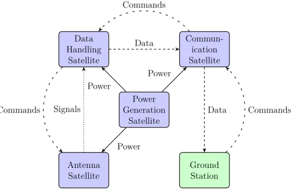
Consider a satellite architecture where only one satellite in a formation is respon-sible for power generation. This satellite could have solar panels, a Radioisotope Thermoelectric Generator (RTG), or other source of power. It could then transfer some of its power to satellites flying in formation. This would mean the other satel-lites would not need a power generation source since the power can be supplied to them remotely. This allows the other satellites to be more specialized for a different purpose. This architecture is illustrated in Fig. 1-2.

Other Applications

Another use of electromagnetic formation flight is maintaining non-Keplerian motion of a satellite. Although the center of mass of a satellite formation using electromag-netic formation flight would move in a Keplerian manner, each satellite would appear to move in a manner that was not governed by Kepler’s laws of motion. Since most satellite orbit estimators rely on Keplerian assumptions, flying in a non-Keplerian

(23)

Power Generation Satellite Commun-ication Satellite Antenna

Satellite GroundStation Data Handling Satellite Power Power Power Signals Data Data Commands Commands Commands

Figure 1-2: Example of a Mission Architecture That Uses Wireless Power Transfer

manner could defeat conventional satellite tracking methods. This would make the satellite difficult to track, which is advantageous from a satellite defense perspective. Fig. 1-3 illustrates a potential orbit where EMFF is used to maintain a non-Keplerian orbit. Satellites A and B maintain a spin about the cross-track direction, keeping formation together using an attractive electromagnetic force between the two. The system center of mass obeys Kepler’s laws, but Satellite A and Satellite B individually appear to move in a manner that is not predictable under Keplerian assumptions.

The electromagnets used for electromagnetic formation flight can also be used to protect the spacecraft from energetic spacecraft radiation. Energetic radiation can damage spacecraft electronics, resulting in data corruption, satellite resets, or even permanent satellite failure [22]. However, active magnetic shielding can be used to deflect the radiation, thus reducing the chances of radiation affecting the spacecraft [23]. By using the electromagnets on the spacecraft, the spacecraft can generate an active magnetic field that would act as a radiation shield for the spacecraft.

(24)

Earth

System Center of Mass Satellite A Satellite B

Figure 1-3: Example of Non-Keplerian Orbits Using EMFF (Not To Scale)

1.1.3 Resonant Inductive Near-Field Generation System

The Resonant Inductive Near-Field Generation System (RINGS) is a testbed that will be used to demonstrate electromagnetic formation flight in a space. RINGS is spon-sored by the Defense Advanced Research Project Agency (DARPA) and is lead by Professor Raymond Sedwick of the University of Maryland. The RINGS are designed to be integrated into the Synchronized Position Hold Engage and Reorient Exper-imental Satellites (SPHERES) testbed, which has been onboard the International Space Station since 2006 [24]–[26]. The combined RINGS and SPHERES system can be seen during an Reduced Gravity Aircraft (RGA) flight in Fig. 1-4. The RINGS sys-tem consists of two units; each unit is an AC electromagnet with supporting control avionics. The specifications of RINGS can be seen in Table 1.1

The RINGS have two general modes: Electromagnetic Formation Flight and Wire-less Power Transfer. In electromagnetic formation flight mode, the units generate a synchronized alternating magnetic field that attracts, repels, and torques the units. Both the amplitude and phase of each unit can be independently controlled. In Wire-less Power Transfer mode, one unit generates an alternating magnetic field while the other "receives" the power by placing a load resistor in line with the circuit, dissipating

(25)

Figure 1-4: RINGS and SPHERES During an RGA Flight

Table 1.1: RINGS Technical Specifications Description Value Number of Units 2 Mean Coil Diameter 0.64 m Number of Turns 100 Max Current (RMS) 18 A EMFF Frequency 83 Hz WPT Frequency 460 Hz Unit Mass 17.1 kg

(26)

the transferred power. While wireless power transfer is a promising new technology, the focus of this work will be on electromagnetic formation flight relating to RINGS.

1.1.4 RINGS Control

To date, all of the work on EMFF control has assumed a fully controllable dipole. In a six degree of freedom environment, this requires three orthogonal coils (or at least three coils where no two are parallel). This allows the magnetic dipole to be pointed in any direction by controlling the amount of current in each coil. For EMFF testbeds on the ground, only two coils were required for a controllable dipole, since the system is limited to three degrees of freedom.

Despite operating in a six degree of freedom environment, RINGS only has one coil per vehicle. This means the dipole is not fully controllable; instead, only the magnitude and the polarity of the coil are controllable by the electromagnet itself. To control the direction of the dipole, the system must be physically rotated. This makes the system non-holonomic, and subsequently makes the control of RINGS more difficult than a holonomic EMFF system.

RINGS control is also difficult because of the proximity of the coil. Previous EMFF work assumed the coils were at least several coil diameters apart. At this distance, the first term of the Taylor series expansion of the force and torque equations is sufficient for describing the system behavior. This "far-field" model is used in nearly all of the previous EMFF research. However, the RINGS will be confined to the SPHERES working volume. This means the RINGS will rarely ever be more than a few coil diameters apart. Therefore, the "near-field" model will need to be used to describe the motion of the RINGS. There is no closed form solution of the "near-field" force and torque model as a function of attitude and separation, making controller development even more difficult. Additionally, the "near-field" model is highly nonlinear with satellite position and attitude.

(27)

1.1.5 Dynamic Programming

Because of the unique and difficult dynamics presenting by RINGS, dynamic program-ming was chosen as the control method for this work. While other control methods can be used [27], dynamic programming was chosen for two main reasons. First, dy-namic programming offers a robustness for nonlinear systems, something that many other control methods do not. Secondly, modeling the RINGS system for a dynamic program requires making less assumptions than other types of controllers.

While dynamic programming is used often in simulation and optimization, it is rarely used for embedded systems. This is most likely because of the large amount of storage space required for the lookup tables generated by dynamic programming. However, this does not mean dynamic programming cannot be applied to embedded systems. The next generation of aircraft collision avoidance uses dynamic program-ming to advise pilots of the optimal action when faced with a potential collision [28]. Neural dynamic programming has also been applied to the tracking, control, and trimming of helicopters [29]–[31].

While Chapters 3 and 4 are specific to the RINGS system, Chapter 2, which discusses the theory behind dynamic programming and approximate dynamic pro-gramming, and Chapter 5, which discusses implementing dynamic programming con-trollers, can be applied to any embedded system. This means that dynamic program-ming is not necessarily limited to RINGS or EMFF. Given the advances in computing power and data compression, dynamic programming may become a more prevalent option for control engineers.

1.2 Previous Work

The previous work discusses in this section pertains to electromagnetic formation flight. The limited amount of previous work on applying dynamic programming to embedded systems is discussed in Section 1.1.4. The previous work completed on mass property identification is discussed in Section 6.1.

(28)

using superconducting electromagnets to maintain a satellite formation in low earth orbit (LEO) [32], [33]. Since then, the Massachusetts Institute of Technology’s Space Systems Laboratory has taken the initiative on EMFF. While a significant amount of work has been done examining EMFF at the systems level [15], [34]–[39], the focus of this literature review will be on the technical aspects of EMFF, namely modeling and simulation, testbed, and control.

1.2.1 EMFF Dynamics

In the thesis by Elias, a non-linear model of EMFF dynamics was developed [40]. This analysis assumed each satellite had a fully controllable dipole. The satellites were also assumed to be separated enough such that the "far-field" assumption held. This "far-field" model assumes the coils are far enough apart such that only the first term of the Taylor series approximation of the force between two coils is sufficient to describe their interaction. The model derived by Elias accounts for electromagnetic forces as well as reaction wheels, the spacecraft bus, and the coupling between the reaction wheels and the spacecraft.

In a thesis by Schweighart, an in-depth model of the intra-satellite forces gener-ated by electromagnets is developed [41]. A "near-field" model is developed for the first time, which describes the forces and torques produced by electromagnetic coils regardless of separation distance. From the "near-field" model, the "far-field" model is then derived and compared against the "near-field" model. Methods for solving the equations of motion are then discussed.

1.2.2 EMFF Testbeds

Under the direction of Professor David Miller, the Massachusetts Institute of Technol-ogy’s Space Systems Laboratory (MIT SSL) has developed several EMFF testbeds. Elias developed an 1 Degree of Freedom (DoF) EMFF testbed which rode on a linear air track [40]. The system consisted of a permanent magnet on a low friction car-riage, which was allowed to move along the linear track, and an electromagnet fixed

(29)

Figure 1-5: Linear Track EMFF Testbed [40]

at the end of the track. The current in the electromagnet was manipulated in order to control the position of the permanent magnet. An ultrasonic ranging device was used to provide position data. The poles of the system could be changed by changing the inclination of the air track. This testbed is seen in Fig. 1-5.

The next testbed was 3 DoF testbed consisting of two vehicles, each with two or-thogonal high temperature superconducting electromagnets [42]. Each vehicle floated on a planer surface using air bearings. The first testbed was originally designed by undergraduates [43], with additional work completed by graduate students [1]. The testbed was able to demonstrate position holds as well as the ability to follow a tra-jectory using EMFF [44]. One of the vehicles, along with Professor Miller, is seen in Fig. 1-61_.

In an investigation of the use of non-superconducting electromagnets for EMFF, Sakaguchi developed the µEMFF testbed [45]. This testbed consisted of two tra-ditional (non-superconducting) electromagnetic coils. One coil was fixed to a servo motor while another was cantilevered from a bar that was allowed to rotate about an air bearing. The attitude of the cantilevered coil was also controlled via a servo mo-tor. The system was able to demonstrate EMFF without the use of superconducting electromagnets. The µEMFF testbed is seen in Fig. 1-7.

(30)

Figure 1-6: Professor David Miller with the 3 Degree of Freedom EMFF Testbed

(a) Conceptual Rendering. (b) Actual System.

(31)

1.2.3 EMFF Control

The first investigation into the control of an electromagnetic formation flight was conducted by Hashimoto, Sakai, Ninomiya, et al. [32], [33]. In their analysis, a two satellite co-planer formation is considered. These satellites maintain an inertially fixed separation distance. The effects of disturbance torques and forces are analyzed for low earth orbit. A phase-shift controller is presented to control the satellite positions. Kong examined the controllability of an EMFF system [35]. The analysis models each electromagnetic field as a stationary multi-pole. The analysis showed that the system is able to control all degrees of translational motion from small perturbations from a nominal position.

In a thesis [46] and series of papers [37], [47]–[49] by Ashun, a non-linear control law is developed for EMFF systems. The controller is designed for a system with any number of satellites. Ashun also shows that, under general assumptions, a multi-satellite formation can be stabilized [47]. Legendre Psedudospectral Methods are used to generate the optimal trajectories, while adaptive control is used to account for the disturbances of Earth’s magnetic field and the errors of the "far-field" EMFF model [48], [49].

In a thesis by Ramirez Riberos, a method for controlling an EMFF system using decentralized control is presented [50]. The control method presented uses a "token" approach where one satellite, which has the "token", is allowed to actuate at a time. The control problem is split into a "high level" and "low level" problem. In the high level problem, the order in which the satellites actuate is determined using dynamic programming. In the lower level problem, a Legendre pseudospectral decomposition approach to find the appropriate actuator control is used.

In a series of papers by Schweighart [39], [51], [52], control methods are presented for a mutli-satellite EMFF formation. Control methods for spinning a satellite array using EMFF are presented [51]. These maneuvers are significant because they would be required for a sparse aperture satellite formation architecture. For other maneu-vers, a method of using Newton’s method combined with the continuation method

(32)

was presented [39], [52]. Since the EMFF dipole solutions are over-determined, a method for choosing the dipole strengths is also presented [52].

In a paper by Cai, Yang, Zhu, et al., methods for finding the optimal trajectory for a satellite formation reconfiguration using EMFF is developed [53]. In their for-mulation, the objective is to minimize the power required to reconfigure a satellite formation using EMFF. Power was chosen as the objective in order to minimize the strain on an EMFF cooling system. Gauss Pseudospectral Methods are used to de-termine the optimal trajectories. In order to implement the trajectories, a trajectory tracking controller is presented that uses both output feedback feedback linearization on an inner control loop and adaptive sliding mode control on an outer loop. The-oretical convergence guarantees for the control are also presented. Simulations are also shown. The simulations show proper trajectory tracking but also show control "chatter" in the dipole solutions.

In a series of papers by Wawrzaszek and Banaszkiewicz, the control of a two satellite planer spinning array is discussed [54], [55]. A linearized model is developed using the "near-field" model of force is developed for two satellites spinning in an array, with the coils axially aligned along the line connecting the two satellites’ center of mass. Stability analysis showed this system is unstable without feedback control. A linear controller is presented that stabilizes the system for a range of disturbances. A three body planer formulation where a third coil is centered between two coils is also presented. The system is shown to be neutrally stable in low earth orbit without control. Using a linear controller, the system is demonstrated to be stabilized for a limited set of disturbances.

In a series of papers by Zhang, Yang, Zhu, et al., a nonlinear control method for docking satellites in six degrees of freedom using EMFF is presented [56], [57]. The "far-field" force and torque model is used to develop a nonlinear system for control. The satellites are assumed to have independent angular control, so only translational control is considered. A controller is developed that uses a linear quadratic regulator around a pre-designed trajectory. The controller was shown in simulation to control a docking of two satellites. The paper is novel in that it is the first to address

(33)

docking of EMFF satellites, but uses the "far-field" model for control development despite operating the "near-field". The paper does not state whether the "far-field" or "near-field" model was used for the dynamics of the simulation.

In a paper by Zeng and Hu, a finite time controller for translational dynamics is presented [58]. A standard "far-field" model is developed and is used for a planer two satellite system. Convergence of the controller in finite, rather than asymptotic, time is proven. The controller was shown in simulation to converge in finite time for multiple scenarios.

(34)

(35)

Chapter 2 Dynamic Programming

The idea of dynamic programming was conceived by Richard Bellman. In his work, Bellman writes "An optimal policy has the property that whatever the initial state and the initial decision are, the remaining decisions must constitute an optimal policy with regard to the state resulting from the first decision" [59]. This is known as Bellman’s

Principle, and is the central idea to dynamic programming. More simply stated, if

an trajectory is known to be optimal, then any sub-trajectory of that trajectory is also optimal.

To illustrate this idea, consider the process illustrated in Fig. 2-1. Each circle is a state, while each line is a path with an associated transition cost. The objective is to move from node A to node F with minimum cost. If the optimal trajectory from A to F is A-C-D-F, then Bellman’s principle states that the optimal trajectory from C is C-D-F. A B C D E F a₁ a₂ b₁ c₁ b₂ c₂ d e

Figure 2-1: Simple Markov Process

(36)

can be found by working backwards from node F. Any trajectory that reaches node F must go through either nodes D or E. The "cost-to-go" from node D to node F is known, as well as the cost-to-go from node E to node F. This step is illustrated in Fig. 2-2(a). Now, the cost-to-go from node B to node F through node D is simply the summation of the transition cost from B to D and the cost-to-go from node D to F. The cost-to-go from B to F going through node E can also be computed in the same manner. The optimal trajectory from node B is simply the trajectory that results in the lowest cost-to-go. The cost-to-go for node C can be found in a similar manner. This step is illustrated in Fig. 2-2(b).

A B C D E F Cost: d Cost: e a₁ a₂ b₁ c₁ b₂ c₂ d e (a) Step 1. A B C D E F Cost: b Cost: e Cost: d Cost: c c= min{c₁ + d, c₂+ e} b= min{b₁+ d, b₂+ e} a₁ a₂ b₁ c₁ b₂ c₂ d e (b) Step 2.

Figure 2-2: Dynamic Programming Analysis of a Simple Markov Process

With the cost-to-go to node F from both B and C known, the cost-to-go from node A to F through node C is the summation of the transition cost from A to C and the cost-to-go from node C to F. This is significant because the cost of all paths from node C to F are not required; rather, only the cost-to-go from C to F is required. The path from A to F through B can also be evaluated in such a manner. The optimal path from A is whichever path that results in minimum cost, determined by Eq. (2.1).

(37)

If a2+ c < a1+ b, then the optimal path from A is the path to C. The optimal path

from C is found in a similar manner, solving min{c1+d, c2+e}. If c1+d < c2+e, then

the optimal path from C is to D and then F. This example illustrates the fundamental principles of dynamic programming.

While it is easy to evaluate all paths for Fig. 2-1, typical dynamic programming problems have many more states, making the possibility of evaluating all paths nearly impossible. The power of dynamic programming is that every path does not need to be evaluated. Instead, the optimal path can be methodically found in reverse, reducing the number of paths evaluated.

2.1 Fundamentals of Dynamic Programming

Let xk be the state of a system at time k. The state equation of a system, seen in

Eq. (2.2), computes the propagation of state xk one time step based on the input uk.

xk+1 = f (xk, uk) (2.2)

In a traditional control sense, the objective of a controller is to minimize the cost function J₀(x₀) = N X k=0 gk(xk, uk, xk+1) (2.3)

where gk(xk, uk, xk+1) is the cost of transitioning from state xk to state xk+1 using

input uk. The cost at time k can be written as

Jk(xk) = gk(xk, uk, xk+1) + Jk+1(xk+1) (2.4) where Jk+1(xk+1) = N X i=k+1 gi(xi, ui, xi+1) (2.5) Jk₊₁(xk+1) is called the cost-to-go from state xk+1, since it is encapsulates the

remain-ing cost of the trajectory. Bellman’s Principle states that if the optimal cost-to-go at time k + 1, written as J∗

(38)

at time k can be solved using Eq. (2.6).

J_k∗(xk) = min

uk∈Uk

gk(xk, uk, f(xk, uk)) + Jk∗+1(f(xk, uk)) (2.6)

Eq. (2.6) is known as Bellman’s Equation and is the basis of dynamic programming. Dynamic programming finds the optimal cost-to-go for a system by using Bellman’s Equation backwards on a trajectory. If the terminal costs J∗

N(xN) are known for all

xN, then JN −∗ 1(xN −1) can be found for all xN −1 by using Bellman’s Equation. Once J_{N −}∗ ₁(xN −1) is known for all xN −1, then JN −∗ 2(xN −2) can be found for all xN −2. This

process can be repeated until J∗

0(x0) is known for all x0. With the optimal cost-to-go

known for all states and times, the optimal input of the system at xk can be found

by solving Eq. (2.7)

u∗_k= arg min

uk∈Uk

gk(xk, uk, f(xk, uk)) + Jk∗+1(f(xk, uk)) (2.7)

The advantage of dynamic programming is that it computes the optimal trajectory for every possible state, meaning dynamic programming converges on the global min-imum of Eq. (2.3). Other control methods, such as Gauss Pseudospectral methods, often do not have the global minimum convergence guarantees that dynamic pro-gramming offers. The convergence guarantees come at the cost of having to compute and store the cost-to-go for every possible state at every time step. While this is done off-line, this can still be cumbersome in terms of both required computational power and required memory. The amount of computation and memory for a dynamic program increases exponentially with the number of states. This is known as the "curse of dimensionality".

One way to reduce the amount of computation and memory required is to late the control problem as an infinite horizon problem. In an infinite horizon formu-lation, the system is assumed to be run for an infinite amount of time. This makes the optimal cost-to-go time invariant, which removes the dimension of time from

(39)

formulation. The cost-to-go for an infinite horizon formulation is seen in Eq. (2.8). J(x₀) = lim N →∞ 1 N N −1 X k=0 gk(xk, uk, xk+1) (2.8)

In anticipation of the large number of states for dynamic programming formula-tions of satellite control problems, the remainder of this work will focus on infinite horizon dynamic programming.

2.2 Dynamic Programming Formulation Types

If an infinite horizon dynamic program is not formulated correctly, the cost-to-go described by Eq. (2.8) can become unbounded, which renders the program unsolvable. There are three general formulations for infinite horizon dynamic programming that provide bounds on Eq. (2.8). They are:

• Discounted Cost

• Stochastic Shortest Path • Average Cost

These formulations are described in Sections 2.2.1 to 2.2.3, respectively.

2.2.1 Discounted Cost

In a discounted dynamic programming formulation, the cost function seen in Eq. (2.8) is adapted by adding a discount factor, α ∈ (0, 1). Using the discount factor, Eq. (2.8) becomes J(x₀) = lim N →∞ 1 N N −1 X k=0 αkgk(xk, uk, xk+1) (2.9)

Assuming that gk(xk, uk, xk+1) ∈ R for all xk, xk+1 ∈ Rn and uk ∈ uk, Eq. (2.9) will

converge finitely [60].

This formulation has the best convergence guarantees out of the three methods discussed in Section 2.2. It also requires the least amount of adaptation when

(40)

con-verting a finite horizon problem into an infinite horizon problem. The downside of a discounted cost formulation is that the trajectories governed by the discounted cost formulation, when compared against trajectories from a stochastic shortest path or average cost formulation, may be sub-optimal.

A discounted cost formulation generally works well with a linear quadratic regula-tor (LQR) cost function, seen in Eq. (2.10). An LQR cost function is quite common in the control field due to its desirable properties of convexity, existence and simplicity of the first derivative, and performance guarantees for linear systems. Let xt be the

target state of the system. The LQR cost function takes the form

gk(xk, uk) = (xk− xt)

>

Q(xk− xt) + u>kRuk (2.10)

where Q and R are positive definite weighting matrices corresponding to state error and control input, respectively. An LQR style cost function would work well with a discounted dynamic programming formulation for regulating a system around a target state. Assuming that all possible states and controls are in the set of real numbers, then the LQR cost function will always be bounded, meaning all trajectories in a discounted DP formulation will have a finite cost.

2.2.2 Stochastic Shortest Path

Consider the Markov process illustrated in Fig. 2-3. In this process, the state of the system is allowed to travel freely between nodes A,B,C,D, and E. However, once the state of the system reaches node T, the system will remain at node T for the remainder of time.

(41)

A

C

B

D E

T

Figure 2-3: Stochastic Shortest Path Markov Process

In a stochastic shortest path dynamic programming formulation, the Markov pro-cess is augmented with a state called the termination state, T. If the transition costs are defined as gk(xk, uk, xk+1) =        gk(xk, uk, xk+1) , xk6∈ T 0, xk∈ T (2.11)

and there is a positive probability of reaching the termination state from any given state, then the cost-to-go will remain bounded [60].

As the name suggests, this type of formulation is best for driving a system to a target set of states via the shortest path. The definition of path will drive the form of the transition cost function. If this objective is to drive the system to a state via the shortest spatial route, then the cost function will be driven by the distances between nodes. If a minimum-time path is desired, then the transition cost will be driven by the transition time between nodes.

The advantage of stochastic shortest path formulations is that it finds the true shortest path between any node and the termination state. Discounted cost formu-lations, when used to find the shortest path to target states(s), may not converge on the actual shortest path. This is because the discount factor reduces the importance of the cost-to-go from a particular node, increasing the weight of transition costs on the state’s cost-to-go. This may result in convergence on a trajectory that is not truly the shortest path.

The disadvantage of stochastic shortest path formulations is the potential exis-tence of improper policy. An improper policy exists when a trajectory from a certain

(42)

state never reaches the termination state. This will cause the trajectory cost to be-come unbounded, resulting in an infinite cost-to-go for certain states. To ensure that the cost-to-go is bounded, there must be a positive probability that the system will reach the termination state from any state.

2.2.3 Average Cost

The average cost formulation can be considered an extension of the stochastic shortest path formulation. Instead of a termination state, there is a recurring state. The goal of the dynamic program is to reduce the average cost of the system, where the cost is reset when the system reaches the recurring state. Unlike the stochastic shortest path formulation, the system may leave the recurring state. The cost-to-go of an average cost formulation is bounded so long as there is a positive probability of reaching the recurrent state from any given state of the system.

2.3 Approximate Dynamic Programming

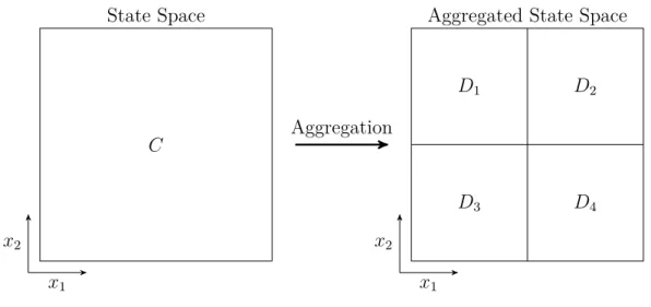
Despite continual advances in computers, many dynamic programs cannot be directly solved due to the shear number of states. However, recent advances in approximate dynamic programming provide approximate solutions for the cost-to-go for a system that cannot be solved using dynamic programming. There are two general ways to solve dynamic programs of large scales: state aggregation and cost approximation. State aggregation is analogous to "lumping" similar states together into an aggregate state, reducing the total number of states of the formulation. Cost evaluation involves approximating the cost function with an basis function. This requires projecting the cost vector into a subspace.

2.3.1 Aggregation

Let C be the set of all possible states of the system. For dynamic programming to be feasible, the state space must be reduced to a finite number of states. Therefore,

(43)

Aggregation

C

D₁ D₂

D₃ D₄

State Space Aggregated State Space

x₁ x₂

Figure 2-4: Illustration of State Aggregation

subsets of points in C are aggregated to make mutually disjoint subsets of C. The state of the system of this formulation becomes i = 0, ..., n, while Di ⊂ C, i =

0, ..., n represent the set of states that the discrete state i represents. The concept of aggregation is illustrated in Fig. 2-4.

This type of formulation transforms a deterministic formulation into a stochastic one. When the system is at state i, the actual state of the system is one of the states in Di. Let pij(u) be the probability of transitioning from aggregate state i

to aggregate state j when input u is applied to the system. Using the framework described in Fig. 2-5, the aggregate state transition probabilities can be computed using Eq. (2.12). pij(u) =X x dixX y pxy(u)ayj (2.12)

There are many ways to define the dissaggregation and aggregation probabilities. The simplest method is called hard aggregation. The hard aggregation technique is equivalent to a nearest-point approximation, where the aggregation probabilities are assigned based on singular aggregate state that encompasses the point. Hard aggregation can be described using Eqs. (2.13a) and (2.13b) and is illustrated in Fig. 2-6(a). dix =        1, x ∈ Di 0, x 6∈ Di (2.13a)

(44)

Aggregate State i System State x Aggregate State j System State y Disaggregation Probabilities dix Transition Probability pxy(u) Aggregation Probabilities ayj Transition Probability pij(u)

Figure 2-5: Aggregation Formulation [60]

1 2

3 4

x₁ x₂

(a) Hard Aggregation.

1 2

3 4

x₁ x₂

(b) Soft Aggregation.

Figure 2-6: Illustration of Aggregation Techniques

ayj =        1, y ∈ Dj 0, y 6∈ Dj (2.13b)

Another aggregation and disaggregation method is called soft aggregation. In soft aggregation, the probabilities are are assigned based on an interpolation of the prob-abilities of the aggregate states. Soft aggregation is illustrated in Fig. 2-6(b).

Bellman’s equation for an aggregate state formulation can be seen in Eq. (2.14).

J∗(i) = g (i, u) + n

X

j=0

pij(u) J∗(j) (2.14)

(45)

to use:

• Value Iteration • Policy Iteration • Linear Programming

Policy iteration and linear programming are better suited problems with a small number of states, while value iteration is more suitable for problems with a large number of states. In anticipation of dealing with a large number of states, value iteration will be the solution method considered here. Let

(T J)(i) = min

u∈U(i)g(i, u) + n

X

j=1

pij(u)J(j) (2.15)

be the mapping of T . Value iteration looks to find the fixed point J∗_{(i) = T J}∗_{(i) for}

all i = 0, ..., n by iterating the mapping T J(i).

J∗(i) = lim k→∞(T

k_J_)(i) _(2.16)

For value iteration to be implemented, the term pij(u)J(j) must be approximated.

If points in Di, i = 0, ..., n are uniformly distributed and sampled q times, pij(u)J(j)

can be approximated by pij(u)J(j) ≈ 1 q q X s=1 J(js) (2.17) where xs ∈ Di (2.18a) f(xs, u) ∈ Djs (2.18b)

The other other adjustment for aggregation methods is if f(xk, uk) /∈ C for all uk ∈ Uk. This happens when the system, by the nature of the dynamics, transitions out

of the state space regardless of the control applied. In this case, the system can be penalized with cost τ. If a stochastic shortest path formulation is used, the system can also transition to the termination state, since the system would terminate anyway.

(46)

The algorithm used for solving the the aggregation formulation is seen in Algo-rithm 1.

Algorithm 1Aggregation Value Iteration Algorithm

Given J0(i)

for k = 0, ..., N do . Run through N iterations

for i= 0, ..., n do . Loop through all aggregation sets

for m= 0, ..., p do . Loop through inputs in U um ∈ U

for s= 1, ..., q do . Run through q samples xk_s ∈ Di . Sample a point in Di xk+1

s = f(xks, um) . Propagate the state equation

ˆgk(s) = g(xks, xks+1, um) .Compute transition cost

if xk_s+1 ∈ C then/ . Check for out-of-bounds

ˆ

Jk(s) = τ . Penalize out of bounds

else ˆ Jk(s) = J(j), where xks+1 ∈ Dj end if end for ˜gk(m) = _p₊₁1 P p

s=0ˆgk(s) .Compute expected transition cost

˜

Jk(m) = _p₊₁1 P p

s=0Jˆk(s) . Compute expected cost-to-go

end for

Jk+1(i) = minm∈(1,..,p)gk(m) + ˜Jk(m) .Evaluate Bellman’s equation

end for end for

2.3.2 Cost Approximation

In cost approximation a basis function, combined with tuning parameters, is used to approximate the cost-to-go of the system. The cost approximation takes the general form of ˜J(φ(x), r), where φ(x) is a basis function that can be computed given state

x, and r is a tuning parameter for the approximation. In the linear case:

˜

J(x, r) = φ(x)r (2.19)

where φ(x) is a row vector and r is a column vector. The key concept of cost ap-proximation is that an apap-proximation for the cost-to-go can be found on-line using state information combined with a set of pre-computed tuning parameters r. The

(47)

true cost-to-go is mapped into the subspace described byφ(x) and r. There are sev-eral different methods to compute the tuning parameters for a linear approximation, including:

• Temporal Difference

• Least Squares Temporal Difference

• Least Squares Policy Evaluation

For this work the linear cost approximation, shown in Eq. (2.19), will be used. The

r vector will be updated according to the least squares temporal differences (LSTD)

method. This method involves simulating a long trajectory and building a matrix C and vector d such that

Cr∗ = d (2.20)

The LTSD finds r∗ _{iteratively using information from the trajectories. As a trajectory}

moves from ik to ik+1, Ck and dk are updated via Eqs. (2.21) and (2.22)

Ck = (1 − δk)Ck−1+ δkφ(ik) (φ(ik) − φ(ik+1))

>

(2.21)

dk= (1 − δk)dk−1+ δkφ(ik)g(ik, ik+1) (2.22)

When a batch of simulations is complete, rk is updated using Eq. (2.23).

rk= Ck−1dk (2.23)

Since the trajectories will eventually terminate, it is necessary to restart the trajecto-ries. To ensure sufficient exploration, a random feasible state is used as the starting state of the system.

Using the LSTD algorithm described in Algorithm 2 the parameter vector r that best matches the cost to go can be found via simulation.

(48)

Algorithm 2Cost Approximation Iteration Algorithm

Given r0

rk = r0

for k = 0, ..., n do .Loop through n iterations

x0 ∈ Ds C−1 = [0] d−1 = [0] i= 0

while i < N do .Run through N samples

ui = arg minu∈U(i)g(xi, f(xi, ui)) + ˜J(φ (f (xi, u)) r)

xi+1= f (xi, ui) . Propagate the state equation δk = _k₊₁1

Ci

k= (1 − δk)Cki−1+ δkφ(xi) (φ(xi) − φ(xi+1))

>

di_k = (1 − δk)dki−1+ δkφ(xi)g(xi)

if xi+1 _{∈ T then} _. _{Check for termination} xi+1 _{∈ D}

s . Restart with a new point

end if

i= i + 1

end while

rk+1 = (CkN)−1dNk

end for

2.4 Applying Dynamic Programming to a Physical

System

While dynamic programming has been used to solve a multitude of complex prob-lems, dynamic programming solutions have rarely been used as a control method for physical systems. The large amount of computation required combined with the large amount of storage space required have hindered dynamic programming’s use on physical systems. With advances in computing and storage, applying dynamic programming to physical systems is becoming a reality. The flow of development for a dynamic programming controller is described in Fig. 2-7.

There are several major considerations when developing a dynamic programming controller. The first is that the physical system needs to be able to be formulated in a dynamic programming formulation with as few states as possible. This will most likely involve mapping the states of the real system into a subspace, performing dynamic programming on the subspace, and mapping the subspace back to the real system. A

(49)

Problem Formulation Aggregation Cost Approx-imation Direct Input Method Rollout Method Cost-to-go _Controller

Figure 2-7: Controller Development Using Dynamic Programming

good understanding of the important versus the non-important states of the system will be required for the problem formulation. It is up to the control engineer to decide which states can be simplified and which must be accounted for.

The finding the cost-to-go for a physical system may also be difficult because the system lives in the real world where an infinite number of states are possible. While approximate dynamic programming maps the infinite number of states into a subspace, it is still up to the control engineer to decide which states are feasible and therefore be accounted for in the cost-to-go. For instance, certain states may be impossible to achieve because of obstructions or physical limitations. Also, there may be certain states that have associated trajectories that take the system out of the state space of the dynamic program. It is again up the control engineer on how to account for these cases. Chapter 4 will present one method for dealing with these problems, but there are multiple ways to address these issues.

More considerations for applying dynamic programming to a control problem are discussed in Section 5.1.

(50)

(51)

Chapter 3 Formulating RINGS as a Dynamic

Programming Problem

While the following two chapters will present novel results for RINGS control, the real purpose of these two chapters are to be a case study for formulating and solving a control problem for a satellite system using dynamic programming. This chapter will discuss specific formulations of the RINGS system that are convenient for dy-namic programming. Chapter 4 will develop solutions of the cost-to-go the specific formulation outlined in Section 3.2.1.

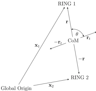
The most fundamental part of the RINGS formulation is the interaction between the two coils. The forces and torques on one electromagnet from the other can be found by integrating the Biot-Savart law, as seen in Eqs. (3.1) and (3.2) [41], where the terms in these equations are defined in Fig. 3-1.

~ F₂ = µ0i1i2 4π I   I ˆr × d~l 1 r3  ×d~l2 (3.1) ~τ₂ = µ0i1i2 4π I ~a₂ ×     I ˆr × d~l 1 r3  ×d~l2   (3.2)

There are no closed form solutions of Eqs. (3.1) and (3.2), so numerical methods will have to be used to approximate Eqs. (3.1) and (3.2).

(52)

~r d~l1 d~l2 ~a₁ ~a₂ i₁ i₂ Coil 1 Coil 2

Figure 3-1: Definition of Two Coils in Proximity

3.1 RINGS Dynamic Programming Formulations

Unlike a simulation built for dynamic programming, which limits the states to those that the dynamic program is concerned about, an embedded system has a set num-ber of real, physical states. To implement dynamic programming on an embedded system, the physical states must be mapped into states that are useful for dynamic programming. This section will map the physical states of RINGS into states that are useful for dynamic programming.

A satellite typically has thirteen standard states, which are grouped into four general categories:

• Position (3 states)

• Velocity (3 states)

• Attitude, measured in quaternions (4 states)

• Angular Rate (3 states)

For a two satellite system, this results in 26 states, which is far too many states for a dynamic programming formulation. However, symmetry in the problem can be used to reduce the number of states in the system.

Dynamic programming applied to electromagnetic satellite actuation

Dynamic Programming Applied to

Electromagnetic Satellite Actuation

by

Gregory John Eslinger

B.S., United States Air Force Academy (2011)

Submitted to the Department of Aeronautics and Astronautics

in partial fulfillment of the requirements for the degree of

Master of Science in Aeronautics and Astronautics

at the

MASSACHUSETTS INSTITUTE OF TECHNOLOGY

June 2013

This material is declared a work of the U.S. Government and is not

subject to copyright protection in the United States

Author . . . .

Department of Aeronautics and Astronautics

May 22, 2013

Certified by. . . .

Alvar Saenz-Otero

Principal Research Scientist

Thesis Supervisor

Certified by. . . .

David W. Miller

Professor of Aeronautics and Astronautics

Thesis Supervisor

Accepted by . . . .

Eytan H. Modiano

Professor of Aeronautics and Astronautics

Chair, Graduate Program Committee

Dynamic Programming Applied to Electromagnetic Satellite

Actuation

by

Gregory John Eslinger

Abstract

Acknowledgments

Contents

List of Figures

List of Tables

Chapter 1

Introduction

1.1

Motivation

1.1.1

Spacecraft Formation Flight

1.1.2

Electromagnetic Formation Flight

1.1.3

Resonant Inductive Near-Field Generation System

1.1.4

RINGS Control

1.1.5

Dynamic Programming

1.2

Previous Work

1.2.1

EMFF Dynamics

1.2.2

EMFF Testbeds

1.2.3

EMFF Control

Chapter 2

Dynamic Programming

2.1

Fundamentals of Dynamic Programming

2.2

Dynamic Programming Formulation Types

2.2.1

Discounted Cost

2.2.2

Stochastic Shortest Path

2.2.3

Average Cost

2.3

Approximate Dynamic Programming

2.3.1

Aggregation

2.3.2

Cost Approximation

2.4

Applying Dynamic Programming to a Physical