HAL Id: hal-00298515
https://hal.archives-ouvertes.fr/hal-00298515
Submitted on 7 Apr 2008
HAL is a multi-disciplinary open access
archive for the deposit and dissemination of
sci-entific research documents, whether they are
pub-lished or not. The documents may come from
teaching and research institutions in France or
abroad, or from public or private research centers.
L’archive ouverte pluridisciplinaire HAL, est
destinée au dépôt et à la diffusion de documents
scientifiques de niveau recherche, publiés ou non,
émanant des établissements d’enseignement et de
recherche français ou étrangers, des laboratoires
publics ou privés.
GLIMS case study of Bering Glacier System, Alaska
M. J. Beedle, M. Dyurgerov, W. Tangborn, S. J. S. Khalsa, C. Helm, B.
Raup, R. Armstrong, R. G. Barry
To cite this version:
M. J. Beedle, M. Dyurgerov, W. Tangborn, S. J. S. Khalsa, C. Helm, et al.. Improving estimation
of glacier volume change: a GLIMS case study of Bering Glacier System, Alaska. The Cryosphere,
Copernicus 2008, 2 (1), pp.33-51. �hal-00298515�
© Author(s) 2008. This work is distributed under the Creative Commons Attribution 3.0 License.
Improving estimation of glacier volume change: a GLIMS case
study of Bering Glacier System, Alaska
M. J. Beedle1,5, M. Dyurgerov2,3, W. Tangborn4, S. J. S. Khalsa1, C. Helm1, B. Raup1, R. Armstrong1, and R. G. Barry1
1National Snow and Ice Data Center, 449 UCB, University of Colorado – Boulder, CO 80309-0559, USA 2Institute of Arctic and Alpine Research, 450 UCB, University of Colorado – Boulder, CO 80309-0450, USA 3Department of Physical Geography & Quaternary Geology, Stockholm University, SE – 106 92 Stockholm, Sweden 4HyMet Inc., 13629 Burma Rd. SW, Vashon Island, WA 98070, USA
5Geography Program, University of Northern British Columbia, 3333 University Way, Prince George, B.C. V2N 4Z9, Canada
Received: 19 June 2007 – Published in The Cryosphere Discuss.: 9 July 2007 Revised: 12 March 2008 – Accepted: 12 March 2008 – Published: 7 April 2008
Abstract. The Global Land Ice Measurements from Space
(GLIMS) project has developed tools and methods that can be employed by analysts to create accurate glacier outlines. To illustrate the importance of accurate glacier outlines and the effectiveness of GLIMS standards we conducted a case study on Bering Glacier System (BGS), Alaska. BGS is a complex glacier system aggregated from multiple drainage basins, numerous tributaries, and many accumulation ar-eas. Published measurements of BGS surface area vary from 1740 to 6200 km2, depending on how the boundaries of this system have been defined. Utilizing GLIMS tools and stan-dards we have completed a new outline (3630 km2) and
anal-ysis of the area-altitude distribution (hypsometry) of BGS using Landsat images from 2000 and 2001 and a US Ge-ological Survey 15-min digital elevation model. We com-pared this new hypsometry with three different hypsome-tries to illustrate the errors that result from the widely vary-ing estimates of BGS extent. The use of different BGS hypsometries results in highly variable measures of volume change and net balance (bn). Applying a simple
hypsometry-dependent mass-balance model to different hypsometries re-sults in a bnrate range of −1.0 to −3.1 m a−1water
equiva-lent (W.E.), a volume change range of −3.8 to −6.7 km3a−1 W.E., and a near doubling in contributions to sea level equiv-alent, 0.011 mm a−1to 0.019 mm a−1. Current inaccuracies in glacier outlines hinder our ability to correctly quantify glacier change. Understanding of glacier extents can become
Correspondence to: M. J. Beedle
comprehensive and accurate. Such accuracy is possible with the increasing volume of satellite imagery of glacierized re-gions, recent advances in tools and standards, and dedication to this important task.
1 Introduction
Glaciers are valuable integrators of their local climate and thus, through their changes, indicators of climate change. Annual field measurements of glacier mass-balance have been undertaken in order to monitor annual change and to understand the relation between glaciers and climate. Such measurements of glacier mass-balance are time consuming, expensive, and arduous. Thus, the vast majority of mass-balance programs intentionally select small, easily accessi-ble, well-defined glaciers with little debris-cover (Fountain et al., 1999). This legacy of studying a small subset of “simple” glaciers has resulted in questionable representation of Earth’s complex mountain glaciers (e.g. Dyurgerov and Meier, 1997; Cogley and Adams, 1998). Indeed, few glaciers conform to the simplistic geographies (morphology and hypsometry) of those with detailed mass-balance studies.
New technology and subsequent techniques have resulted in many recent studies using remote sensing to study a broader spatial range of glaciers (e.g. Arendt et al., 2002; Larsen et al., 2007). Such studies have compared two or more measures of glacier surface height, typically separated on decadal time scales, resulting in vertical height change, volume loss or gain, and an average net balance (bn) rate for
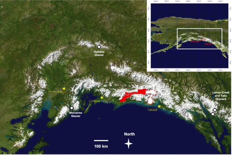
Fig. 1. Location of Bering Glacier System, Alaska.
Bering Glacier System (BGS) is shaded in red. The two meteorological stations used in the PTAA model, Cordova and Yakutat (yellow stars), are indicated to the west and east of BGS. The four glaciers with temporally significant mass-balance records in southern and southeast Alaska, which were tested as possible benchmark glaciers, are also indicated (white and black bordered diamonds). Malaspina Glacier is outlined in red just east of BGS.
Braithwaite and Zhang, 1999; Tangborn, 1999; and Paul et al., 2002) in order to extend our understanding of glacier change beyond the few glaciers with detailed annual field studies. Whether we compare remotely sensed glacier sur-faces to derive surface height change or use models of glacier mass-balance the glacier surfaces being assessed must be lat-erally constrained, or, in other words, extent of the glaciers must be outlined. Accurate glacier outlining is perhaps the most basic of glacier measurements, but one of significant importance. A glacier’s outline yields measurements of face area and length; and, when projected to a horizontal sur-face and combined with a digital elevation model (DEM), an outline leads to a glacier’s distribution of area with elevation (hypsometry). Perhaps most importantly, a glacier’s outline defines the surface area with which any measure of surface height change or mass-balance will be integrated to obtain an estimate of a glacier’s bn. Errant glacier outlines result in
in-accurate measures of glacier volume change and bn(Arendt
et al., 2006; Raup et al., 2006). Unfortunately, the seemingly simple task of accurately outlining a glacier meets with many complications.
Complications which hinder an accurate outline include different definitions of what should be included as glacier within an outline and the exceeding complexity of many glacier systems. In this paper we address these two com-plications by 1) illustrating the facility of a common glacier definition developed by and utilized for the Global Land Ice Measurements from Space (GLIMS) project, and 2) applying this glacier definition to a study of mass-balance and volume change of the complex Bering Glacier System (BGS), Alaska (Figs. 1 and 2).
1.1 This study
The GLIMS project at the National Snow and Ice Data Cen-ter, University of Colorado (Raup et al., 2006, 2007; Raup and Khalsa, 2006) is creating standardized methodology and
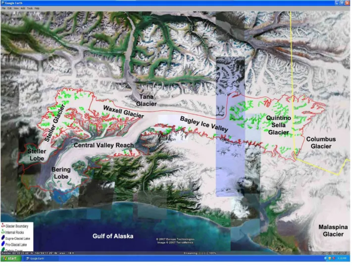
Fig. 2. Bering Glacier System.
Glacier outlines digitized in GLIMSView displayed in Google EarthTM. Surging Bering Glacier System (SBGS) and Steller Glacier (includ-ing Steller Lobe) are outlined in red. Together the SBGS and Steller Glacier comprise the Ber(includ-ing Glacier System. Nunataks are outlined in light green and debris-cover is outlined in dark green. The yellow line is the border between Alaska (west) and Yukon Territory, Canada (east).
tools, and a common glacier database through which the sci-entific community can pursue more accurate and more acces-sible knowledge of glacier characteristics and change, lead-ing to better monitorlead-ing of the world’s glaciers in regards to past, present, and future climatic change. This study, within the broader GLIMS project, aims to address the importance of accurate glacier outlining and hypsometry creation – es-pecially in regards to large, complex glaciers – as well as to demonstrate the facility of GLIMS methodology and tools. To do so we compare the results achieved when integrating net balance estimates (from three different models) with four different BGS hypsometries. In addition we examine charac-teristics such as debris-cover, surge dynamics, and multiple flow divides, which complicate studies of glacier extent and change.
The comparisons within this study yield: 1) an illustration of the importance of accurate glacier outlining via a common, or at least explicitly stated, glacier definition; 2) accurate, transparently-defined outlines and hypsometries of BGS; 3) a discussion of BGS mass-balance and volume change re-sults for the second half of the 20th century from three mod-els; and 4) a discussion of some of the problems facing the glaciological community in regards to accurately outlining and understanding some of the world’s major glaciers. 1.2 Bering Glacier System
Previous studies have noted the complexity of BGS. In their preliminary inventory of Alaska glaciers, Post and Meier (1980) use BGS as “a particularly extreme example.”
Table 1. Official Bering Glacier System nomenclature.
This table describes some of the Official (US Board on Geographic Names) Bering Glacier System (BGS) nomenclature that often leads to confusion when defining the component parts of BGS.
Name Description
Bering Glacier Entire piedmont lobe (Bering Piedmont Glacier), including Steller and Bering Glacier Piedmont Lobes Steller Lobe Portion of piedmont lobe fed by Steller Glacier
Steller Glacier Tributary feeding Steller Lobe
Central Medial Moraine Band Moraine covered ice between Steller and Bering Lobes Bering Lobe Portion of piedmont lobe fed by the main trunk glacier Central Valley Reach Central portion of main trunk glacier feeding Bering Lobe Bagley Ice Valley Main accumulation area both east and west
Waxell Glacier West branch of Bagley Ice Valley
Bering Glacier System Entire glacier flowing to the Bering Piedmont Glacier
It is in and between two countries (USA, Canada), two major drainages (Pacific, Chitina-Copper), and two major mountain ranges, (Chugach and St. Elias Mountains). Fur-thermore, the main glacier drainage system has at least five differently named component areas (Steller, Bering, Colum-bus, Quintino Sella Glaciers, and Bagley Ice Field), and esti-mates of its total area range from 1740 to 6200 km2 depend-ing on how the “Berdepend-ing Glacier” is defined.
Molnia and Post (1995) present a history of the exploration and study of BGS, a history including early explorers nam-ing portions of the same glacier individually, as a view of the entire glacier was not possible at the time. This history has led to “the nomenclature associated with [BGS being] con-fusing.” Some history clarifies how this has come about, and is a sobering reminder of the relative infancy of our ability to view larger glaciers in their entirety.
During the late 19th and early 20th centuries a number of expeditions to the region described and mapped portions of BGS. In 1880 the US Coast and Geodetic Survey named the Bering Glacier in honor of Captain Vitus Bering, an 18th century Danish sea captain. However, the vast expanse of the upper reaches of BGS was not recognized until many years later. In the intervening years, expeditions in the re-gion named portions of BGS. For example, an expedition in 1897 lead by the Duke of the Abruzzi on Mt. St. Elias, named a portion of BGS after Christopher Columbus, and a con-siderable tributary to the Columbus Glacier as the Quintino Sella Glacier after a renowned Italian alpinist (Fig. 2). It was not until 1938, when Bradford Washburn made the first aerial photographs of BGS that a complete view was obtained of the large upper elevation glacier complex that feeds the sprawling piedmont lobe (Molnia and Post, 1995).
Official (US Board on Geographic Names) BGS nomen-clature was championed by Austin Post in a significant effort to accurately preserve the history and honor vital crewmem-bers of Vitus Bering’s voyage. Table 1 presents a portion of the official BGS nomenclature that often leads to confusion when defining the component parts of BGS.
Recently, remote sensing, via aerial photography and satellite imagery, has afforded analysts the means of visual-izing, outlining and quantifying the entirety of BGS. Unfor-tunately confusion still lingers. Previous outlines have incor-porated different portions of BGS. Reported surface areas of BGS range from 1740 km2upwards to 6200 km2, with vari-ous measurements in between (Post and Meier, 1980; Molnia and Post, 1995; and Arendt et al., 2002). Note that all glacier definitions and measures of extent for BGS are commonly labeled as Bering Glacier. Bering Glacier officially refers to only the entire piedmont lobe fed by Steller Glacier and main trunk glacier (Central Valley Reach) flowing down from the Bagley Ice Valley (Fig. 4). For this study we outlined the individual glaciers that comprise BGS. For the purposes of studying individual glacier mass-balance and dynamics we divide BGS into two individual glaciers: 1) Steller Glacier (including Steller Lobe), and 2) the portion of BGS that con-tributes to the Bering Lobe, or, that part of BGS that surges or the “surging Bering Glacier System” (SBGS) (Figs. 3 and 8). Such a subdivision allows the analyst the freedom to study one glacier individually or the entire BGS.
The official (US Board on Geographic Names) and oft-published surface area of 5173 km2makes BGS the largest glacier in Alaska1. To put this behemoth in perspective BGS (by this measure) is nearly as large as all the glaciers in Scan-dinavia and the Alps combined (5287 km2) (Dyurgerov and Meier, 2005).
Recent work (Arendt et al., 2002) has concluded that shrinking Alaska glaciers comprise the largest glacier con-tribution to global sea level rise yet measured. A few mas-sive coastal glaciers (including BGS) are the biggest con-tributors. Accurate quantification of contributions to sea level rise begins with accurate glacier outlines, which lead 1The US Board on Geographic Names lists Bering Glacier Sys-tem (BGS) as having an area of 5173 km2, which is used here as the official area. BGS, according to Molnia and Post (1995), is 5174 km2.
Table 2. Description of glacier definitions used for four outlines.
This table includes the component glacier portions used to uniquely define the four glacier outlines used in this study.
Name Description
Arendt (A) outline Outline including Bering Lobe, portions of the Central Medial Moraine Band, Central Valley Reach and a portion of eastern Bagley Ice Valley
Surging Bering Glacier System (SBGS) outline
Outline of the surging portion of Bering Glacier System including Bering Lobe, portions of the Central Medial Moraine Band, Central Valley Reach, Bagley Ice Valley, Quintino Sella Glacier and a portion of Columbus Glacier
Bering Glacier System (BGS) outline
Outline of the entire Bering Glacier System including Bering Glacier, Steller Glacier, Central Medial Moraine Band, Central Valley Reach, Bagley Ice Valley, Quintino Sella Glacier and a portion of Columbus Glacier, but excluding all nunataks
Bering Glacier System –
nunataks included (BGS+N) outline
Outline of the entire Bering Glacier System as described above for BGS, but including all nunataks
to measurements of surface area – over which surface height change and mass-balance measurements are integrated. Un-fortunately an accurate, consensus measure of BGS surface area has not been realized in recent publications.
2 Data and methods
This study uses four different BGS outlines (Table 2 and Fig. 3) combined with a US Geological Survey (USGS) DEM to create four hypsometries. Three methods of mod-eling mass-balance are used with the four hypsometries to illustrate the potential errors resulting from different glacier outlines.
2.1 Outlines
The four outlines are discussed here in order from smallest to largest. The first outline was used in a previous study while the remaining three outlines were created for this study. These four outlines were chosen or created to represent a range of outlined areas using different glacier definitions. We also outlined debris-cover for each of the four glacier outlines in order to investigate the impacts of debris-cover on glacier mass-balance. Refer to Table 2 and Fig. 3 for abbreviated descriptions and images of these outlines.
2.1.1 Arendt (A) outline
The first outline was used by Arendt et al. (2002) (A) and yields a total surface area of 2193 km2. The A outline was digitized from 1972 USGS topographical maps. It should be noted that this outline knowingly encompasses “considerably less than the total area of the [BGS’s] hydrological basin” as the outline includes only ice deemed to be well represented by laser altimetry survey flights of 1995 (Arendt et al., 2002,
supporting online text; Arendt, 2007, personal communica-tion). The A outline is included here as a representative of the lower end of the range of previous estimates of BGS surface area.
2.1.2 Surging Bering Glacier System (SBGS) outline The SBGS outline includes all ice that contributes to the por-tion of the BGS piedmont lobe that surges. All nunataks are excluded. The SBGS outline has a surface area of 3630 km2. 2.1.3 Bering Glacier System (BGS) outline
The Bering Glacier System (BGS) outline includes all ice within the official US Board on Geographic Names definition of BGS (Table 1). All nunataks are excluded. This outline includes Steller and Bering Piedmont Lobes (Bering Glacier) and all ice that contributes to it. The BGS outline has a sur-face area of 4373 km2.
2.1.4 Bering Glacier System – nunataks included (BGS+N) outline
The Bering Glacier System – Nunataks Included (BGS+N) outline is identical to the BGS outline, but includes all nunataks. The BGS+N outline has a surface area of 4796 km2, and roughly follows the glacier definition of Mol-nia and Post (1995) (see detailed discussion in Sect. 4.1.2). We have included all nunataks in this outline to attempt to replicate this glacier definition that results in the official BGS surface area (5173 km2) and to illustrate the importance of
accounting for nunataks when mapping glaciers. 2.1.5 Debris-cover (DC) outlines
Debris-cover (DC) outlines were digitized in order to em-ploy a simple model that incorporates the hypsometry of DC
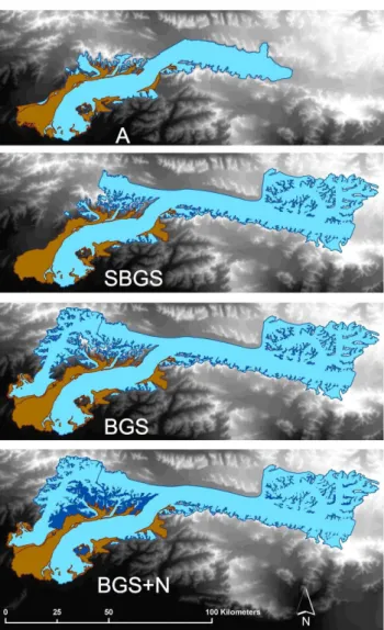
Fig. 3. Glacier outlines.
These four panels display the Arendt (A), Surging Bering Glacier System (SBGS), Bering Glacier System (BGS), and Bering Glacier System – nunataks included (BGS+N) outlines. Glacier and nunatak polygons are outlined in dark blue. Ice and snow sur-faces are light blue. Debris-cover is outlined in dark brown and colored light brown. Dark blue areas in the bottom (BGS+N) panel are nunataks.
ice and the insulating effects of this debris. DC ice extent varies depending upon the glacier outlines discussed above. The naming scheme used in this study is DC followed by the glacier outline acronym. The DC-A is 481 km2, the DC-SBGS is 561 km2and the DC-BGS and DC-BGS+N are both 624 km2.
2.2 Outlining methods
Here we describe the glacier definition used to outline SBGS followed by a discussion of the methodology used to cre-ate the SBGS, BGS, BGS+N and DC outlines. The glacier
definition and outlining standards used here were also used to digitize outlines for Steller Glacier and other glaciers in southern and southeast Alaska (Beedle, 2007).
2.2.1 SBGS glacier definition
Different glacier definitions will be employed depending upon the intent of a study. Here we discuss in detail the glacier definition of SBGS as an example.
SBGS is outlined here with the intent of being used to quantify the “iceshed” contributing to a unique terminus – Bering Lobe. While Bering Lobe is a portion of Bering Glacier (piedmont lobe) it surges and responds to climate change independently of the adjacent Steller Lobe (Fig. 4). In order to understand surges and climatic responses of these unique termini an outline of the contributing ice sheds must be used. The SBGS outline includes Bering Lobe, the SBGS portion of the Central Medial Moraine Band, Central Val-ley Reach, BagVal-ley Ice ValVal-ley (including Waxell Glacier), Quintino Sella Glacier, and a portion of Columbus Glacier (Fig. 2). The composite parts of SBGS can also be thought of as the larger BGS without Steller Glacier, Steller Lobe, and a small portion of the Central Medial Moraine Band deemed attributable to flow from Steller Glacier. In essence SBGS simply incorporates all portions of BGS except Steller Glacier and its tributaries. The outlined extent comprises all ice that contributes to a common terminus (Bering Lobe) with the intention of being used in studies of glacier mass-balance, and adheres to the GLIMS glacier definition devel-oped to reduce inconsistencies in glacier treatment (Raup and Khalsa, 2006).
More specifically, the glacier definition elaborated on in the GLIMS Analysis Tutorial and employed here, includes 1) ice bodies above bergschrunds that contribute ice and snow to the glacier, 2) connected stagnant ice masses even when supporting an old-growth forest, and 3) all debris-covered ice. Excluded are 1) all nunataks, 2) steep rock walls that avalanche snow onto the glacier, 3) all continuous, adja-cent ice masses which contribute to a terminus other than the Bering Lobe (e.g. Steller, Tana, and Malaspina Glaciers), 4) detached, hanging ice masses that may contribute ice via avalanching, and 5) adjacent snowfields, which do not con-tribute to the mass of BGS. While these standards are sug-gested by GLIMS and utilized in this study, the ultimate glacier definition is to be determined by the analyst, based on objectives and nature of the study. The definition em-ployed here is used in order to discern an individual glacier within a complex glacier system. The reader is directed to the complete GLIMS discussion of glacier definition and analy-sis standards within the GLIMS Analyanaly-sis Tutorial2.
Outlining the terminus of SBGS necessitates a decision on the inclusion or exclusion of certain levels of glacier 2http://www.glims.org/MapsAndDocs/guides.html (Raup and Khalsa, 2006)
Fig. 4. Bering Glacier piedmont lobe.
This GLIMSView screen image displays the Landsat 7 ETM+ panchromatic band (10 September 2001) used to outline the termini of Bering Glacier System. The Steller Glacier is outlined in yellow and part of Surging Bering Glacier System is shown outlined in white. Nunataks are outlined in green. Bering Glacier officially refers to the large piedmont lobe which includes the Steller Lobe, Central Medial Moraine Band, Bering Lobe and Central Valley Reach.
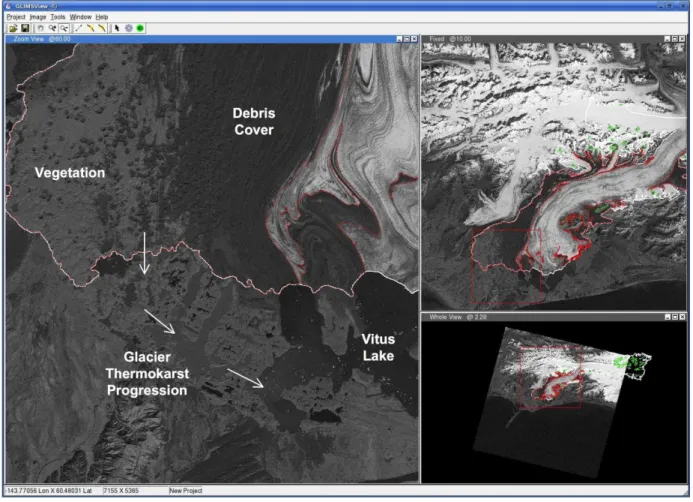
thermokarst (Fig. 5), although no standard has been proposed by GLIMS. Stagnant, debris-covered ice bodies, still in con-tact with the parent glacier, slowly disintegrate via progres-sion of glacier thermokarst; first, growth of debris contin-ues, second, moulins and crevasses develop into sinkholes and then into large water-filled depressions, third, only rem-nant ice cores remain (Benn and Evans, 1998). In the case of BGS termini, glacier thermokarst progression reaches a mature stage when melt pools erode into one another form-ing distinctive terminal lakes (e.g. Vitus Lake), definitively delimiting the receding glacier’s terminus. At what stage of glacier thermokarst should an adjacent ice body no longer be included as part of the parent glacier? Outlining the en-tire area of debris-covered, stagnant ice (all levels of glacier thermokarst included) results in an unchanging terminus po-sition, until the main body of the glacier recedes from the stagnant ice mass, then a large “jump” in glacier recession will be noted. For SBGS, BGS and BGS+N it was decided to
digitize the termini at the mature stage of glacier thermokarst. Defining a mature glacier thermokarst boundary is subject to the analyst’s perception of the continuum of conditions of glacier thermokarst, but serves to provide a progression of terminal disintegration until a definitive terminus can be out-lined.
2.2.2 SBGS, BGS and BGS+N outlining
The SBGS, BGS and BGS+N outlines created for this study were derived from two Landsat 7 ETM+ images (obtained from the Global Land Cover Facility http://glcf.umiacs.umd. edu/). The first image (acquired 31 August 2000)) was used to digitize the accumulation area. The second image (10 September 2001) was used to digitize the ablation area. Nei-ther image alone covers the entirety of BGS.
Outlining was done manually using GLIMSView, “A cross-platform application intended to aid and standardize the process of glacier digitization for the GLIMS project”
Fig. 5. Surging Bering Glacier System debris-cover.
This GLIMSView screen image displays the Landsat 7 ETM+ panchromatic band (10 September 2001) used to outline the termini of the Bering Glacier System. The three panels progress (counterclockwise from lower right) from a whole view of the entire Landsat 7 ETM+ scene to a zoom view of the western portion of the Bering Lobe. The Surging Bering Glacier System is outlined in white and the area defined as debris-cover is outlined in red. Nunataks are outlined in green. Note the large glacierized area covered by vegetation (lighter grey), the continuity of debris-cover, and the progressive stages of glacier thermokarst.
(Raup et al., 2007). GLIMSView is freely available on the GLIMS website (http://www.glims.org). Previous work (e.g. Paul, 2001; Albert, 2002) has been done on the accuracy of automated techniques, utilizing manual outlines as a known, accurate benchmark. We used manual outlining to achieve the most-accurate outline possible considering the complex-ity of BGS, which includes significant debris-cover, forest cover and numerous, complex flow divides. Other studies (e.g. Williams et al., 1991, 1997; Hall et al., 2003) have in-vestigated errors inherent in outlining glaciers due to compli-cations such as differing ice facies and image resolution, with a focus on accurately delimiting glacier termini from space. In this study, we focus more on errors that stem from glacier definition of large, complex glacier systems (such as BGS), because glacier definition is found to play an extremely im-portant role, with potential errors of hundreds to thousands km2.
USGS topographic maps were used to visually determine glacier “ice sheds”, particularly to define flow boundaries be-tween SBGS and the adjacent Steller, Tana, Baldwin, and Malaspina Glaciers. Further refinement and validation of the outline was done by visual analysis of linear surface fea-tures indicative of glacier flow. This task was aided by band stretching (Landsat 7 ETM+ bands 4, 3, and 2) within the his-togram function of GLIMSView, particularly in the largely featureless accumulation areas (Fig. 6).
2.2.3 DC outlining
We outlined DC from the 10 September 2001 Landsat 7 ETM+ scene, using the same methodology discussed above. All areas of DC with continuous (uninterrupted by any visi-ble ice) debris or vegetation cover, including areas of glacier thermokarst, are defined as DC (Fig. 5). This definition of DC was chosen for the purpose of delimiting the area that
Fig. 6. Steller Glacier and Surging Bering Glacier System flow divide.
This GLIMSView screen image shows the flow divide between Steller Glacier and the Waxell Glacier part of Surging Bering Glacier System. The image is a composite of Landsat 7 ETM+ bands 4, 3, and 2 (31 August 2000) ‘stretched’ within the histogram function of GLIMSView (see inset). The snow covered glacier surfaces are predominantly purple. Such stretching helps to visualize linear surface features indicative of glacier flow (indicated by small white arrows). The Surging Bering Glacier System outline is in white.
might be significantly impacted by a reduction of ablation due to a sufficiently thick debris-cover (discussed below). 2.3 DEM and hypsometry creation
To create glacier hypsometries we used each of the outlines to “clip” a 1972 15-min USGS DEM. Each glacier or DC hypsometry is comprised of the total area within every 50 m elevation bin over the outlined elevation range (Fig. 9). The 1972 USGS DEM is derived from 1:63 360 scale topographic maps (USGS, 1993). The aerial photography used to create the 1972 DEM was taken in various years between the 1950s and early 1970s. This DEM has been used in other studies (e.g. Arendt et al., 2002; Muskett et al., 2003) and has been noted as a source of potential error when deriving glacier sur-face height change. Muskett et al. (2003) estimated the 1972 DEM to range from 9±27 m too low to 4±3 m too high, depending upon site and the potential errors of the modern DEMs used as vertical control.
2.4 Mass-balance models
We use three mass-balance models to illustrate the variabil-ity of glacier mass-balance and volume change that can result from different glacier outlines. Each of these models relies on accurate measures of glacier hypsometry, DC area, ac-cumulation area ratio (AAR) and/or glacier shape to model mass-balance.
2.4.1 PTAA mass-balance and volume change
The Precipitation Temperature Area-Altitude (PTAA) model uses precipitation and temperature records from distant lower altitude stations plus a glacier’s hypsometry to model mass-balance (Tangborn, 1999). The PTAA model output (Fig. 10) used in this study is an average (1950–2004) rate of balance change for each 50 m elevation bin (termed mass-balance gradient here), derived from Cordova and Yaku-tat, Alaska (Fig. 1) meteorological records and the SBGS
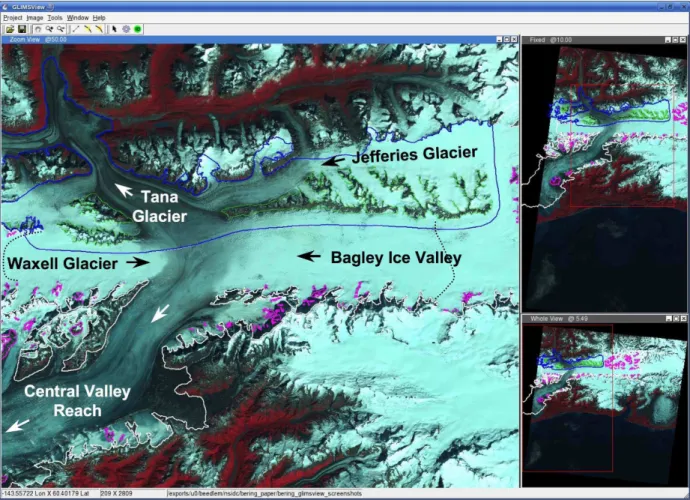
Fig. 7. Tana Glacier and Surging Bering Glacier System divide.
This GLIMSView screen image shows the complex flow divide between the Tana Glacier and Surging Bering Glacier System (SBGS). The three panels progress from a whole view of the entire Landsat 7 ETM+ scene (31 August 2000) (lower right) to a zoom view of the Tana/SBGS divide (left). Vegetation appears red. Tana Glacier is outlined in blue and Tana Glacier nunataks are outlined in green. SBGS is outlined in white with nunataks outlined in purple. Approximate location of the PTAA modeled 1500 m ELA is shown by black dotted lines on Bagley Ice Valley and Waxell Glacier. Compare these to the visible transient snow lines, which are at approximately 1200 m.
hypsometry (Fig. 9). Field measurements by Fleisher et al. (2005) found an average ablation rate (1998–2005) near the terminus of SBGS (below 100 m) of approximately
−10 m a−1which corresponds well with the PTAA modeled (1950–2004 average) ablation rate of between −10.8 m a−1
at sea level and −10.0 m a−1at 100 m. In situ measurements of accumulation are not available to validate the PTAA mod-eled mass-balance in the accumulation zone (additional dis-cussion below).
2.4.2 Debris-cover adjusted PTAA mass-balance and vol-ume change
In order to investigate the possible impact of DC on mass-balance and volume change, we adjusted the PTAA mass-balance gradient to reflect attenuated melting of DC ice resulting in a much flatter balance gradient for DC areas. This reduction in ablation is achieved by integrating DC hypsometry (Fig. 9)
with the adjusted PTAA balance gradient (Fig. 10). Then this DC total is added to the integration of the original PTAA bal-ance gradient and the hypsometry of debris-free ice, yielding a total, DC-adjusted bnand volume change.
It is assumed here that the outlined DC is composed of a debris mantle that is sufficiently thick (>5–10 cm) to insulate the underlying ice and significantly reduce ablation (Fig. 5). Ablation rates of DC ice drop dramatically with an increase in DC thickness greater than 1 cm to 2 cm (e.g. Nakawo and Rana, 1999; Benn and Evans, 1998). In this study the ad-justment for DC ice ablation is assigned to be one-quarter of the PTAA modeled mass-balance, thus significantly reduc-ing ablation for the DC areas. The intent is to investigate the possible significance of outlining and accounting for DC in remote sensing studies of mass-balance of glaciers with sig-nificant DC. The appropriateness of this assigned reduction in ablation under a DC mantle is discussed further below.
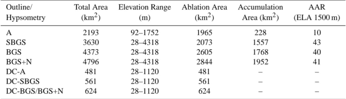
Table 3. Geographic statistics of four glacier outlines.
Total area, elevation range, ablation area, accumulation area and accumulation area ratio (AAR) statistics for the Arendt (A), Surging Bering Glacier System (SBGS), Bering Glacier System (BGS) and Bering Glacier System – nunataks included (BGS+N) outlines and their associated debris-covered (DC) areas.
Outline/ Total Area Elevation Range Ablation Area Accumulation AAR
Hypsometry (km2) (m) (km2) Area (km2) (ELA 1500 m)
A 2193 92–1752 1965 228 10 SBGS 3630 28–4318 2073 1557 43 BGS 4373 28–4318 2605 1768 40 BGS+N 4796 28–4318 2844 1952 41 DC-A 481 28–1120 481 – – DC-SBGS 561 28–1120 561 – – DC-BGS/BGS+N 624 28–1120 624 – –
2.4.3 Template method mass-balance and volume change A third method of modeling mass-balance, the template method (Dyurgerov, 1996; Khalsa et al., 2004), is used here to illustrate the importance of outlined glacier shape on estimates of mass-balance and volume change. The tem-plate method relies upon the relation between glacier mass-balance and AAR. A nearby “benchmark” glacier with an-nual, in situ, surface mass-balance measurements is selected as representative of other glaciers in a climatically homoge-nous region. The relation between mass-balance and AAR from the benchmark glacier is applied to the hypsometry of the glacier in question. Here we use the average (1950–2004) AAR of each outline to obtain an average mass-balance based upon the relation between mass-balance and AAR at a representative benchmark glacier. Of particular importance is the proximity of the benchmark glacier and the assump-tion that this nearby glacier realistically represents the re-gion’s climate. Taku, Lemon Creek, Gulkana and Wolverine Glaciers (Fig. 1) (the only glaciers in southern and southeast Alaska with temporally significant mass-balance records) were tested as possible benchmarks for the BGS area. Us-ing either Wolverine or Gulkana Glacier (both with similar distances from and closer to BGS) as the benchmark yields nearly identical results. The Gulkana Glacier is used here be-cause the in situ measurements agree best with laser altimetry studies (Arendt et al., 2002) as well as being best correlated with modeled BGS bn (r=0.62)3. Correlation coefficients
between modeled BGS bn and the other in situ records are
0.45 (Lemon Creek Glacier), 0.38 (Taku Glacier), and 0.37 (Wolverine Glacier).
3This modeled BGS b
nwas derived via the PTAA model
(Tang-born, 1999), but annually for the period 1950 to 2000, as opposed to the 1950–2004 average bnused in this study, and is included in
Dyurgerov and Meier (2005).
3 Results
3.1 Geographical statistics of outlines
Each of the three outlines created for this study has an ele-vation range of 28 to 4318 m, and a DC eleele-vation range of 28 to 1120 m. Refer to Table 3 for complete geographical statistics.
SBGS, as defined and outlined here from 2000 and 2001 imagery, is 3630 km2, which is 1543 km2or 30% less than the official BGS area (5173 km2). Nunataks outlined and
ex-cluded from the SBGS outline (Fig. 3) total 123 km2or 3% of SBGS area. The DC-SBGS outline has an area of 561 km2, 15% of the total SBGS area.
Possible variability in outlining the complex SBGS was estimated to not exceed ±330 km2, or 9% of total SBGS area. This error estimate accounts for different possible outlines within glacier thermokarst, debris and vegetation cover of the piedmont lobe (Fig. 4), errant divide assessment (Figs. 6 and 7), divide migration during surges, and inclusion or ex-clusion of nunataks. Additional details on these estimates are discussed below.
BGS, as outlined here from 2000 and 2001 satellite im-agery, is 4373 km2, which is 800 km2or 15% less than the official 5173 km2. Nunataks outlined and excluded from the BGS outline total 423 km2or 10% of BGS area (Fig. 3). The DC-BGS outline has an area of 624 km2, 14% of the total BGS area.
BGS+N is 4796 km2, which is 377 km2 or 7% less than the official 5173 km2. BGS+N includes all nunataks within the BGS outline (Fig. 3). The DC-BGS+N has an area of 624 km2, 13% of the total BGS+N area. The BGS+N outline was digitized using the same glacier definition that resulted in the official BGS area (5173 km2). Below we discuss
pos-sible reasons why BGS+N differs from this official area. Dividing the accumulation and ablation areas by the PTAA modeled average ELA of 1500 m (discussed below) results in AARs of 10, 43, 40, and 41 (percent accumulation area) for
Fig. 8. Surging Bering Glacier System.
Looking north-northeast on the Surging Bering Glacier System outline digitized in GLIMSView and displayed in Google EarthTMwith a 3 fold vertical exaggeration. The glacier outline is in red, nunataks are outlined in light green, and debris-cover is outlined in dark green.
the A, SBGS, BGS and BGS+N outlines respectively. Steady state AARs generally are between 50 and 80, with typical values between 55 and 65, and glaciers with debris-covered termini generally have lower AARs (<40) (Benn and Evans, 1998). The AAR of 10 for the A outline is extremely low, while the remaining AARs of 43, 40 and 41 are more rea-sonable, especially when considering the significant area of debris-cover on the lower reaches of BGS.
3.2 Mass-balance and volume change
Highly variable measures of bn and volume change result
from the use of different glacier outlines and resultant hyp-sometries (Table 4). Integration of the four hyphyp-sometries with modeled mass-balance results in a bnrange of −1.0 to
−4.2 m a−1, and volume change of −3.8 to −9.6 km3a−1. All bnand volume change results are in units of water
equiv-alent unless otherwise noted.
Use of the PTAA model with the four hypsometries re-sults in the greatest net mass loss. PTAA bnrates range from
−1.9 to −4.2 m a−1and volume change rates from −6.8 to
−9.6 km3a−1.
Adjusting the PTAA modeled mass-balance for DC results in a significant decrease in net mass loss, with the ranges of bn results changing to −1.0 to −3.1 m a−1 and volume
change to −3.8 to −6.7 km3a−1. Note that this adjustment for the effects of DC results in volume loss being reduced by over 3 km3a−1.
Use of the template method results in estimates of bnand
volume change similar to that of the DC-adjusted PTAA model with bnranging from −1.2 to −3.0 m a−1and volume
Fig. 9. Hypsometries of four Bering Glacier System outlines.
Area-altitude distribution (hypsometry) of the Arendt (A), Surging Bering Glacier System (SBGS), Bering Glacier System (BGS) and Bering Glacier System – nunataks included (BGS+N) and the debris-covered area associated with each. Each line plots total glacier surface area within 50-m elevation bins.
4 Discussion
4.1 Geographical statistics
Geographical statistics (Table 3) from the outlines created for this study are significantly different from those published previously. Here we discuss potential errors in defining and outlining BGS, why disparities exist between measures of BGS surface area, and implications of these results.
4.1.1 Potential errors of BGS outlines
The complex divide between BGS and Tana Glacier (Fig. 7) heavily influences our estimated error of ±330 km2(9% to-tal glacier area). Different outlines of this single flow di-vide may vary by as much as ±200 km2. Previous outlines of BGS may have included the entirety of Bagley Ice Val-ley, unrealistically diminishing Tana Glacier’s accumulation area. The estimated error of ±330 km2includes this uncer-tainty, and therefore may be too large.
The greatest likelihood of errors in the outlining of BGS stems from measurement difficulties of the accumulation area. Snow cover at upper elevations hinders accurate de-tection of glacier outlines. Adjacent snowfields, which do not contribute to glacier flow, may erroneously be included. Such errors serve to increase the accumulation area, result-ing in higher AAR values, and more positive mass-balance measurements.
Another likely source of error exists when outlining near ridge crests on steep, shaded slopes. Outlining in these ar-eas may include steep snow covered rock slopes that con-tribute to glacier mass-balance via avalanching, or negate ar-eas masked by shadow. These arar-eas are extremely small rel-ative to total glacier area, and assumed here to be negligible. 4.1.2 Disparities between different BGS outlines
Why do published BGS areas differ by a factor of three? Pri-marily this is caused by disparate glacier definitions. Sec-ondary causes of such disparities include errors that stem from the use of different methods employed for outlining, and actual changes in glacier extent.
Even when a common definition is not used to create glacier outlines, transparent understanding of the glacier’s extent can be realized through the explicit statement of the employed definition. Molnia and Post (1995) provide such a definition for the BGS outline that results in the official pub-lished surface area of 5173 km2.
We define the Bering Glacier system based on drainage-basin analysis, divide topography, ice-surface moraine pat-terns, and ice elevation and flow lines. We include: all of the Steller Glacier, virtually all of the Bagley Icefield (including the Quintino Sella Glacier, but excluding a small northward-flowing section of the icefield that feeds the Tana Glacier and an unnamed distributary draining north to Logan Glacier), and the area described by the [US] Board [on Geographic
Fig. 10. PTAA modeled mass-balance gradients.
Average (1950–2004) mass-balance gradient from the PTAA model (blue squares) and the debris-cover adjusted mass-balance gradient (brown circles).
Names] as the ‘Bering Glacier’ in 1932. (Molnia and Post,
1995; p. 98).
Via this definition of BGS we know that this outline in-cludes Steller Glacier (Fig. 2), which we find to be 743 km2, and deem to be separate from the SBGS portion of BGS. It is uncertain whether the Molnia and Post (1995) outline in-cludes or exin-cludes nunataks, but it likely included them, as the resultant area is significantly larger than our BGS out-line. We find the area within the BGS glacier boundary that is nunatak to be 423 km2. Excluding nunataks is likely the primary reason why our definition of BGS results in an area, which is 800 km2less.
Another, separate BGS definition, is that of Arendt et al. (2002) (A), which results in a surface area of 2193 km2 (Fig. 3). This glacier definition is discussed in regards to both BGS and Malaspina Glacier (Fig. 1):
Our outlined areas for these two glaciers are consider-ably less than the total area of their glacierized hydrological basins, because we terminated the outlines at the uppermost elevation contours that our profiling sampled. (Arendt et al.,
2002; online supporting text p. 6).
Such an outline results in very little accumulation area, an unrealistic AAR, and increased negative mass-balance (Ta-bles 3 and 4). It should be mentioned here that the Arendt et
Fig. 11. PTAA modeled daily transient snow line.
PTAA modeled daily transient snow line (TSL) for 2000 (light blue) and 2001 (black). The imaging dates of the Landsat 7 ETM+ scenes used in this study are labeled. Note that the highest TSL elevation occurs in mid-August, followed by a rapid decrease in elevation due to modeled snowfall in late August and early-September.
al. (2002) study was of regional mass-balance and that “the uppermost areas of these glaciers are accounted for in the St. Elias regional extrapolation, based on data from nearby glaciers” (Arendt et al., 2002; online supporting text p. 6).
Use of different methods to map glaciers can also result in errors. Digitization of glacier outlines can either be done manually or via an array of automated techniques (e.g. Al-bert, 2002). Manual digitization is still the most accurate tool for extracting accurate glacier outlines, but is also te-dious and time consuming (e.g. Raup et al., 2007). While automated techniques are rapid and consistent, they can fal-ter with regards to ambiguous surfaces, particularly the de-lineation of DC (e.g. Whalley and Martin, 1986; Sidjak and Wheate, 1999). All of the outlines used in this study were digitized manually.
BGS terminus retreat and advance may be a primary rea-son for disparities between the ablation areas of the A out-line (digitized from 1972 maps) and the SBGS, BGS and BGS+N outlines (digitized from 2000 and 2001 imagery). BGS surge dynamics, which have resulted in dramatic ter-minus advance followed by rapid retreat, have driven sur-face area changes of greater than 100 km2(Molnia and Post, 1995). Surges (1957–1960, 1965–1967, and 1993–1995) fol-lowed by terminus retreat occurred between the aerial pho-tography (1950s to 1970s) on which the A outline is based, and the 2000 and 2001 satellite imagery used for the other outlines in this study.
4.1.3 Largest glacier in the United States?
BGS (frequently referred to as Bering Glacier) is often listed as the largest glacier in the United States at 5173 km2, with the neighboring Malaspina Glacier (Fig. 1) number two with
Table 4. Mass-balance, volume change and sea level equivalent results.
Average annual mass-balance, volume change and sea level equivalent for the period 1950 to 2004 from three models (PTAA, DC-adjusted and Template method). Results are presented for the Arendt (A), Surging Bering Glacier System (SBGS), Bering Glacier System (BGS) and Bering Glacier System – nunataks included (BGS+N) outlines.
Model Units A SBGS BGS BGS+N
PTAA bn (m a−1W.E.) −4.2 −1.9 −2.1 −2.0
Volume Change (km3a−1W.E.) −9.3 −6.8 −9.0 −9.6
Sea Level Equivalent (mm a−1) 0.027 0.019 0.026 0.028
DC-adjusted bn (m a−1W.E.) −3.1 −1.0 −1.3 −1.3
Volume Change (km3a−1W.E.) −6.7 −3.8 −5.6 −6.2
Sea Level Equivalent (mm a−1) 0.019 0.011 0.016 0.018 Template Method bn (m a−1W.E.) −3.0 −1.2 −1.3 −1.3 Volume Change (km3a−1W.E.) −6.6 −4.4 −5.9 −6.4
Sea Level Equivalent (mm a−1) 0.019 0.013 0.017 0.018
an area of 5000 km2 (Molnia, 2001). Our SBGS, BGS, BGS+N areas of 3630 km2, 4373 km2 and 4796 km2 re-spectively may seem to alter this statistic, but measures of Malaspina Glacier suffer from the same complications of glacier definition as those discussed above for BGS. The greater Malaspina Glacier system has also been historically composed of numerous, separately named glaciers, includ-ing Columbus, Seward, Agassiz, and Malaspina Glaciers, all of which comprise the larger glacier system. Previous esti-mates of Malaspina Glacier area typically include the portion of the massive piedmont lobe attributable to Agassiz Glacier. Using the same general glacier definition and methodology employed to derive the SBGS outline results in a Malaspina Glacier area of 3220 km2, significantly smaller than even the SBGS.
4.2 Bering Glacier System volume change
Our results show wide-ranging differences in estimates of BGS volume change, depending upon variability among out-lines and mass-balance models (Table 4). Here we firstly discuss variability that is due solely to different outlines and resultant hypsometry, then variability attributable to the dif-ferent methods of modeling mass-balance, and finally, impli-cations of these results.
4.2.1 Variability due to different outlines and resultant hyp-sometries
In this section we use only DC-adjusted modeled mass-balance results (Table 4) to illustrate variability that stems from different glacier outlines. We find bn results varying
from −1.0 to −3.1 m a−1and average volume change rang-ing between −3.8 to −6.7 km3a−1, depending upon glacier outline variability alone. This is not surprising, but simply illustrates the importance of accurate glacier outlines,
espe-cially with regard to recent efforts to accurately discern con-tributions of mountain glaciers to sea level equivalent (SLE). The A outline, with an extremely low AAR of 10, not sur-prisingly results in the most negative bn, the greatest volume
loss and the greatest contribution to SLE. SBGS results in the least negative bn, least volume loss and the least contribution
to SLE.
Accurate glacier outlines are obviously extremely impor-tant to our understanding of the volume change and mass-balance of any glacier. Indeed, BGS outline variability plays a greater role in determining mass-balance estimates than the mass-balance models utilized in this study.
4.2.2 Variability due to different mass-balance models The three mass-balance models used in this study provide different results, all of which are negative, regardless of glacier outline or model (Table 4). Each of these models has unique assumptions, which highlight the importance of accu-rate glacier outlines and differently impact results. Here we discuss the variability of these results, the assumptions that lead to these results and make some comparisons with previ-ous studies. To do so we utilize the results for only SBGS, which has a bn range of −1.0 to −1.9 m a−1 and a volume
change range of −3.8 to −6.8 m a−1.
The PTAA model results in the most negative
bn (−1.9 m a−1) and the greatest volume change
(−6.8 km3a−1). Reliance upon distant, sea-level
mete-orological stations (Fig. 1) likely biases this model towards more negative mass-balance results, especially in such a topographically extreme region where precipitation will be highly variable, and may be significantly greater at upper elevations. Different studies have shown very high annual precipitation in the St. Elias Mountains. Mayo (1989) cites National Weather Service data of 2 to 6 m mean annual precipitation and the PRISM map (Daly et al., 1994) for Alaska and Yukon Territory, Canada indicates that BGS
accumulation area receives between 5 and 13 m of precip-itation annually. Thus, it is possible that the PTAA model underestimates accumulation. Tangborn (1999) found the PTAA model to reveal a more-negative cumulative bn than
the field measured cumulative bnof South Cascade Glacier,
Washington, due to the models “much greater ice ablation on the lower glacier.” With field measurements (Fleisher et al., 2005) of BGS ablation corroborating PTAA modeled ablation we hypothesize that the more-negative PTAA bias likely stems from underestimation of accumulation. However, other studies (Tangborn, 1997, and Tangborn and Post, 1998), find PTAA simulated accumulation balance to agree within 0.2 m for point measurements over a 5-year period on Columbia Glacier, Alaska. PTAA modeled ELA values may also reflect an underestimation of accumulation. Observed transient snow lines (TSL) in the two Landsat 7 ETM+ images used in this study reveal an approximate elevation of 1200 m for both scenes (Fig. 7), while the PTAA models TSL as 1513 m on 31 August 2000 and 1350 m on 10 September 2001 (Fig. 11). Daily TSL elevations from the PTAA model reveal that uppermost elevations are realized in mid-August in both 2000 and 2001, suggesting that late-August or September imaging may be too late to capture end of ablation season conditions on BGS, or that the PTAA model overestimates TSL elevation. The 1950–2004 average ELA used in this study (1500 m) may be too high. Additional in situ observations are needed to understand accumulation and transient snow line of BGS, originating in the topographically significant St. Elias Mountains.
The DC-adjusted model results in less negative bn
(−1.0 m a−1) and volume change (−3.8 km3a−1). This is due to the significant attenuation of ablation assigned to the 561 km2of DC, illustrating that the insulating effects of DC can be extremely important in assessments of mass-balance of glaciers with significantly DC areas (Fig. 5). The DC ad-justment assigned here results in a 3.0 km3a−1reduction in volume loss when compared with the PTAA modeled results. Arendt et al. (2002, online supporting text, p. 6) found thinning rates on the Malaspina Glacier piedmont lobe to be similar on both DC ice and nearby clean ice areas at the same elevation, and therefore included the DC ice of BGS in their volume change estimates without sampling this area. This result contradicts our debris-cover ablation rate assump-tions, suggesting that debris-cover (at least that which was characterized by the portion of Malaspina Glacier sampled in Arendt et al., 2002) may not have a significant impact on ablation rates, or that emergence velocity hindered detection of ablation when assessing surface height change.
Using the relative surface elevation of the DC of Central Medial Moraine Band (higher) and the adjacent bare ice of Bering and Steller Lobes (lower), Austin Post (personal com-munication, 2007) estimated the DC ice to have an ablation rate roughly half that of the adjacent clean ice. This ablation estimate is less negative than our assumed DC ablation rate of one-quarter of clean ice ablation rates.
Kayastha et al. (2000) find a 40 cm thick DC to reduce ablation rates by one-third, and negligible ablation rates for a DC greater than one meter. This result suggests that our outlined DC area (Fig. 5) must be in excess of 40 cm thick for our estimated ablation rate of one-quarter that of clean ice to be valid. In situ validation is needed to confirm our assumptions of DC thickness and attenuation of ablation.
While not fully understood, it is revealed here that accurate assessment of DC ablation rates, and accurate outlining of DC, is imperative in studies of volume change on glaciers with significant DC.
Template method estimates of SBGS mass-balance are also less negative than the PTAA model results with a bnof
−1.2 m a−1and volume change of −4.4 km3a−1, very sim-ilar to those from the DC-adjusted PTAA model. Assump-tions within the template method that may impact the accu-racy of these estimates include benchmark glacier proximity, climatic regime, glacier shape/hypsometry, and possible er-rors in BGS AAR estimates derived from the PTAA modeled ELA.
Gulkana Glacier, used here as the benchmark for the BGS area, is located approximately 350 km north north-west in a continental climatic zone (Fig. 1). The Gulkana Glacier mass-balance record correlates best with annual, PTAA mod-eled SBGS mass-balance. In addition, template method bn
for the A (−3.0 m a−1) compares well with the bnfound by
Arendt et al. (2002) for the period 1995–2000 (−2.8 m a−1)4. Regardless of such favorable comparisons, it seems implausi-ble that such a distant, continental glacier would serve well as a benchmark for mass-balance of the maritime BGS. Using the maritime Wolverine Glacier as the benchmark, however, yields template method modeled BGS results nearly identical to those that employ Gulkana Glacier as the benchmark. This may be due to the importance of glacier shape in the tem-plate method and the similar wedge-shape of both Gulkana and Wolverine Glaciers.
The shape of a glacier revealed via an accurate outline and quantified by its hypsometry will impact how glaciers within a common climatic region integrate climatic inputs, and thus will respond differently (Furbish and Andrews, 1984). Gulkana Glacier is generally wedge-shaped – with area in-creasing with elevation, whereas SBGS is more rectangular, with similar surface area regardless of elevation. A wedge-shaped glacier will preferentially weight the larger upper ele-vation accumulation areas, whereas a rectangular glacier will equally weight the evenly distributed areas, thus an identical AAR will not necessarily result in common mass-balance. For example, within the template method, the SBGS AAR of 43 (resulting from a 1500 m ELA) is assigned to have a bn resulting from an AAR of 43 on the Gulkana Glacier;
however it is unlikely that the relation between bnand AAR
4Presented as an ice equivalent in Arendt et al. (2002) of
−3.1 m a−1. A conversion to water equivalent results in an approx-imate bnof −2.8 m a−1.
will be identical on glaciers with different shapes. The use of Gulkana Glacier as a benchmark for SBGS may have re-sulted in slightly less negative mass-balance results, as the relation between Gulkana Glacier bn and AAR will reflect
the preferential weighting of upper elevation areas due to its shape.
The USGS DEM used in this study is a source of signif-icant error in all three models. Errors arise from the ques-tionable accuracy of the DEM, especially over the largely featureless accumulation areas, and various dates of aerial photography. Using an unchanging glacier surface to model mass-balance through time introduces large uncertainties, as any elevation – mass-balance feedback is negated. This may be especially significant on BGS due to significant ice dis-placement during recent surge events from 1957–1960, from 1965–1967, and from 1993–1995 (Molnia and Post, 1995).
The three models utilized in this study have individual as-sumptions inherent to each, with different impacts upon ac-curacy. Due to such assumptions and associated possible errors, we favor the estimates of volume change and mass-balance from the DC-adjusted PTAA model as the most plau-sible. Based upon this model we find SBGS bn to have
av-eraged −1.0 m a−1with volume change of −3.8 km3a−1for the period 1950–2004.
4.2.3 Implications
Our estimates of contributions to SLE (using the DC-adjusted model) range from 0.011 mm a−1to 0.019 mm a−1 (Table 4), or from 0.59 mm to 1.03 mm for the period 1950 to 2004, depending on glacier outline. This illustrates how accurate understanding of mountain glacier contributions to SLE is dependent upon accurate glacier outlines.
Previous studies (Arendt et al., 2002; Larsen et al., 2007) have illustrated the dramatic net mass loss from Alaska glaciers and associated contributions to SLE. Arendt et al. (2002) find BGS volume change to be −1.5 km3a−1from 1972 to 1995 and −5.97 km3a−1from 1995 to 2000, result-ing in a total net mass loss of −64.8 km3for the period 1972 to 2000. Using our DC-adjusted model and the same out-line (A) used by Arendt et al. (2002) (Fig. 3) over the period 1972 to 2000 we find volume loss of −5.8 km3a−1and cu-mulative volume loss of −156.6 km3, well over double the total net mass loss found by Arendt et al. (2002). The DC-adjusted modeled rate of volume loss for the period 1972 to 2000 (−5.8 km3a−1) is similar to the rate found by Arendt et
al. (2002) for the period 1995 to 2000 (−5.97 km3a−1). This
leads us to the hypothesis that previous results for the early period (1972–1995) may have underestimated volume loss. Such an underestimation could stem from errors in the 1972 USGS DEM and the 1993–1995 surge (Molnia and Post, 1995), which redistributed a large amount of volume to lower elevations, likely having a significant impact on emergence just prior to measurement in 1995. Note that this comparison of measured (Arendt et al., 2002) and modeled mass-balance
(this study) uses a common outline (A) and thus the varying results are due to the differences between and shortcomings of the measurement and modeling methods. Using our DC-adjusted model and the SBGS outline over the period 1972 to 2000 we find volume loss of −2.6 km3a−1and total volume loss of −70.2 km3. This is less than half the total volume loss found using the same model and the A outline, a huge differ-ence resulting entirely from glacier definition and outlining.
Larsen et al. (2007) find that glacier thinning in southeast Alaska is about double that of the Arendt et al. (2002) study due primarily to an under-representation of calving glaciers. While our results are for only one glacier system, it is pos-sible that previous measures (Arendt et al., 2002) underesti-mate contributions to SLE from Alaska glaciers, echoing the conclusions of other studies (Larsen et al., 2007). The dis-parity between our results and those of Arendt et al. (2002), however, is due to the differences between laser altimetry of glacier surface height change and mass-balance models as opposed to complications with regional extrapolation from a limited set of altimetry profiles.
5 Conclusions
Using accurate glacier outlines and hypsometries is impera-tive to understanding mass-balance, volumetric change, eu-static sea level rise, and relationships between changes in such measures and climate. To illustrate this point, we have used the complex BGS as a case study. Mass-balance re-sults for four different BGS outlines show widely differing results in bn, volume change, and contributions to SLE.
Out-line variability alone (using our DC-adjusted model) results in a bnrange of −1.0 to −3.1 m a−1, a volume change range
of −3.8 to −6.7 km3a−1, and a near doubling in contribu-tions to SLE, 0.011 mm a−1to 0.019 mm a−1. Such
variabil-ity, in the case of BGS, stems primarily from the use of dif-ferent glacier definitions.
The surface area of the BGS is found here to be 4373 km2, significantly less than the official area of BGS (5173 km2).
We favor dividing BGS into its two component glaciers (Steller Glacier and SBGS) allowing analysts to study ei-ther glacier individually or the larger BGS. This division re-sults in a definition of SBGS, which we find to be 3630 km2. This new outline and associated hypsometry, when inte-grated with the DC-adjusted PTAA model, result in SBGS mass-balance of −1.0 m a−1 and an annual volume change of −3.8 km3a−1 for the period 1950–2004. Accuracy of these results is dependent upon the shortcomings of the DC-adjusted PTAA model, which include potential underestima-tion of accumulaunderestima-tion at upper elevaunderestima-tions, reality of the as-signed attenuation of ablation under mapped DC area and accuracy and use of the single DEM.
In order to understand change of complex glacier systems, and what is causing these changes, it is imperative that we be-gin with accurate glacier outlines. While BGS is an extreme
case study, it is likely that the lack of an accurate outline extends to other large, important glaciers in Alaska and be-yond. This point is illustrated here by our preliminary mea-sure of Malaspina Glacier surface area, which we find to be 3262 km2, significantly less than the frequently published 5000 km2 (Molnia, 2001). Utilization of GLIMS tools and techniques will help in future assessment of glacier extents and change.
The GLIMS project’s methods, tools, and database, which were employed for this study, serve to standardize glacier definition, provide a user-friendly digitization tool (GLIMSView), and make glacier outlines (and subsequent geographical statistics) widely available to potential analysts via a common database. Utilization of these GLIMS stan-dards will result in a much-improved understanding of the extent of the world’s glaciers, assessment of how and why they are changing, and potential human impacts stemming from such changes (such as eustatic sea level rise).
It is imperative that glaciologists continue to study mass-balance of large complex glaciers and glacier systems, which represents a significant advance when compared with the legacy of detailed studies on small, simple, supposedly rep-resentative glaciers. To do so, however, we must begin with accurate glacier outlines. Such outlines will be a valuable platform from which we can gain a much more accurate un-derstanding of glacier extents, changes in extent, drivers of such changes, and implications of these changes.
With increasing satellite imagery coverage of glacierized regions, advances in tools such as GLIMSView and employ-ment of GLIMS standards there is no reason why our under-standing and inventory of glacier outlines and hypsometries should not be comprehensive and accurate.
Acknowledgements. We greatly appreciate significant
contri-butions by A. and R. Post to the discussion of Bering Glacier System nomenclature and history, as well as their very helpful additional comments and suggestions. Thanks are due to A. Arendt for generously providing one of the outlines used in this study and for a greatly appreciated, diligent review. We would like to thank R. Williams and an anonymous reviewer for helpful suggestions, and D. Hall for patience and assistance as editor. Thank you to P. J. Fleisher for willing contributions of in situ ablation measurements. GLIMS at NSIDC is supported by NASA award NNG04GF51A.
Edited by: D. Hall
References
Albert, T.: Evaluation of remote sensing techniques for ice-area classification applied to the tropical Quelccaya ice cap, Peru, Po-lar Geog., 26(3), 210–226, 2002.
Arendt, A. A., Echelmeyer, K. A., Harrison, W. D., Lingle, C. S., and Valentine, V. B.: Rapid wastage of Alaska glaciers and their contribution to rising sea level, Science, 297, 382–386, 2002.
Arendt, A., Echelmeyer, K., Harrison, W., Lingle, C., Zirnheld, S., Valentine, V., Ritchie, B., and Druckenmiller, M.: Updated esti-mates of glacier volume changes in the western Chugach Moun-tains, Alaska, and a comparison of regional extrapolation meth-ods, J. Geophys. Res., 111, F03019, doi:10.1029/2005JF000436, 2006.
Beedle, M. J.: GLIMS glacier database. Boulder, CO: National Snow and Ice Data Center/World Data Center for Glaciology, Digital Media, 2007.
Benn, D. I. and Evans, D. J. A.: Glaciers and glaciation, Arnold Publishers, New York, NY, 1998.
Braithwaite, R. J. and Zhang, Y.: Modelling changes in glacier mass balance that may occur as a result of climate changes, Geogr. Ann. A, 81(4), 489–496, 1999.
Cogley, J. G. and Adams, W. P.: Mass balance of glaciers other than the ice sheets, J. Glaciol., 44(147), 315–325, 1998.
Daly, C., Neilson, R. P., and Phillips, D. L.: A statistical-topographic model for mapping climatological precipitation over mountainous terrain, J. Appl. Meteorol., 33(2), 140–158, 1994. Dyurgerov, M.: Substitution of long-term mass-balance data by
measurements of one summer, Z. Gletsch., 32, 177–184, 1996. Dyurgerov, M. B. and Meier, M. F.: Mass balance of mountain and
subpolar glaciers: a new global assessment for 1961–1990, Arct. Alp. Res., 29(4), 379–391, 1997.
Dyurgerov, M. B. and Meier, M. F.: Glaciers and the changing earth system: A 2004 snapshot, Institute of Arctic and Alpine Re-search, University of Colorado, Occasional Paper No. 58, 2005. Fleisher, P. J., Bailey, P. K., Natel, E. M., Miller, J. R., and Tracy,
M. W.: Post-surge field measurements of ablation and retreat, eastern sector, Bering Glacier, Alaska, Abstracts with program, Geol. Soc. Am., 37, 7, 423, 2005.
Fountain, A. G., Jansson, P., Kaser, G., and Dyurgerov, M.: Sum-mary of the workshop on methods of mass balance measure-ments and modeling, Tarfala, Sweden August 10–12, 1998. Ge-ogr. Ann. A, 81(4), 461–465, 1999.
Furbish, D. J. and Andrews, J. T.: The use of hypsometry to indicate long-term stability and response of valley glaciers to changes in mass transfer, J. Glaciol., 30(105), 199–211, 1984.
Hall, D. K., Bayr, K. J., Sch¨oner, W., Bindschadler, R. A., and Chien, J. Y. L.: Consideration of errors inherent in mapping his-torical glacier positions in Austria from the ground and space (1893–2001), Rem. Sens. Environ., 86, 566–577, 2003. Kayastha, R. B., Takeuchi, Y., Nakawo, M., and Ageta, Y.:
Practi-cal prediction of ice melting beneath various thickness of debris-cover on Khumbu Glacier, Nepal, using a positive degree-day factor, Debris-covered glaciers, proceedings of a workshop held at Seattle, Washington, USA, September 2000, IAS Publ. no. 264, 71–81, 2000.
Khalsa, S. J. S., Dyurgerov, M. B., Khromova, T., Raup, B. H., and Barry, R. G.: Space-based mapping of glacier changes using ASTER and GIS tools, IEEE T. Geosci. Rem., 42(10), 2177– 2183, 2004.
Larsen, C. F., Motyka, R. J., Arendt, A. A., Echelmeyer, K. A., and Geissler, P. E.: Glacier changes in southeast Alaska and north-west British Columbia and contribution to sea level rise, J. Geo-phys. Res., 112, F01007, doi:10.1029/2006JF000586, 2007. Mayo, L. R.: Advance of Hubbard Glacier and 1986 outburst of
Russell Fiord, Alaska, USA, Ann. of Glaciol., 13, 189–194, 1989.
Molnia, B.: Glaciers of Alaska, Alaska Geographic, 28, 2, 2001. Molnia, B. F. and Post, A.: Holocene history of Bering Glacier,
Alaska: A prelude to the 1993–1994 surge, Phys. Geogr., 16(2), 87–117, 1995.
Muskett, R. R., Lingle, C. S., Tangborn, W. V., and Rabus, B. T.: Multi-decadal elevation changes on Bagley Ice Valley and Malaspina Glacier, Alaska, Geophys. Res. Lett., 30(16), 1857, doi:10.1029/2003GL017707, 2003.
Nakawo, M. and Rana, B.: Estimate of ablation rate of glacier ice under a supraglacial debris layer, Geogr. Ann. A, 81(4), 695–701, 1999.
Paul, F.: Evaluation of different methods for glacier mapping using Landsat TM, EARSeL Workshop on Remote Sensing of Land Ice and Snow, Dresden, June 16–17, 2000, EARSeL eProceedings, 1, 239–245, 2001.
Paul, F., Maisch, M., Rothenbuhler, C., Hoelzle, M., and Haeberli, W.: Calculation and visualization of future glacier extent in the Swiss Alps by means of hypsographic modelling, Global Planet. Change, 55, 343–357, 2002.
Post, A. and Meier, M. F.: A preliminary inventory of Alaskan Glaciers. Proceedings of the Riederalp Workshop, September 1978, IAS-AISH Publ. No. 126, 45–47, 1980.
Raup, B. and Khalsa, S. J. S.: GLIMS analysis tutorial, available at: www.glims.org/MapsAndDocs/guides.html, 2006.
Raup, B., Rocoviteanu, A., Khalsa, S. J. S., Helm, C., Armstrong, R., and Arnaud, Y.: The GLIMS geospatial glacier database: A new tool for studying glacier change, Global Planet. Change, 56, doi:10.1016/j.gloplacha.2006.07.018, 2006.
Raup, B., K¨a¨ab, A., Kargel, J. S., Bishop, M. P., Hamilton, G., Lee, E., Paul, F., Rau, F., Soltesz, D., Khalsa, S. J. S., Beedle, M., and Helm, C.: Remote sensing and GIS technology in the Global Land Ice Measurements from Space (GLIMS) project, Comput. Geosci., 33, 104–125, 2007.
Sidjak, R. W. and Wheate, R. D.: Glacier mapping of the Ille-cillewaet icefield, British Columbia, Canada, using, Landsat TM and digital elevation data, Int. Jour. Remote Sens., 20, 273–284, 1999.
Tangborn, W. V.: Using low-altitude meteorological observations to calculate the mass balance of Alaska’s Columbia Glacier and relate it to calving and speed, in: Calving Glaciers: Report of a Workshop, February 28–March 2, 1997, edited by: Van der Veen, C. J., BPRC Report No. 15, Byrd Polar Research Center, The Ohio State University, Columbus, Ohio, 141–161, 1997. Tangborn, W. V.: A mass-balance model that uses low-altitude
me-teorological observations and the area-altitude distribution of a glacier, Geogr. Ann. A, 81(4), 753–765, 1999.
Tangborn, W. V. and Post, A. P.: Iceberg prediction model to reduce navigation hazards: Columbia Glacier, Alaska. Ice in Surface Waters, Volume 2, Proceedings of the 14th International Sym-posium on Ice, Potsdam New York, 17–31 July 1998.
United States Geological Society, United States Department of the Interior, Digital elevation models: data users guide 5, 1993. Whalley, W. B. and Martin, H. E.: The problem of hidden ice in
glacier mapping, Ann. Glaciol., 8, 181–183, 1986.
Williams Jr., R. S., Hall, D. K., and Benson, C. S.: Analysis of glacier facies using satellite techniques, J. Glaciol., 37(125), 120–128, 1991.
Williams Jr., R. S., Hall, D. K., Sigurdsson, O., and Chien, J. Y. L.: Comparison of satellite-derived with ground-based measure-ments of the fluctuations of the margins of Vatnaj¨okull, Iceland, Ann. Glaciol., 24, 72–80, 1997.