Predicting maize phenology : intercomparaison of functions for developmental response to temperature

HAL Id: hal-02636120

https://hal.inrae.fr/hal-02636120

Submitted on 27 May 2020

HAL is a multi-disciplinary open access archive for the deposit and dissemination of sci-entific research documents, whether they are pub-lished or not. The documents may come from teaching and research institutions in France or abroad, or from public or private research centers.

L’archive ouverte pluridisciplinaire HAL, est destinée au dépôt et à la diffusion de documents scientifiques de niveau recherche, publiés ou non, émanant des établissements d’enseignement et de recherche français ou étrangers, des laboratoires publics ou privés.

Distributed under a Creative Commons Attribution - NonCommercial - NoDerivatives| 4.0

Predicting maize phenology : intercomparaison of

functions for developmental response to temperature

S. Kumudini, F.H. Andrade, K.J. Boote, G.A. Brown, K.A. Dzotsi, G.O.

Edmeades, T. Gocken, M. Goodwin, A.L. Halter, G.L. Hammer, et al.

To cite this version:

S. Kumudini, F.H. Andrade, K.J. Boote, G.A. Brown, K.A. Dzotsi, et al.. Predicting maize phenol-ogy : intercomparaison of functions for developmental response to temperature. Agronomy Journal, American Society of Agronomy, 2014, 106 (6), pp.2087-2097. �10.2134/agronj14.0200�. �hal-02636120�

Biometry, Modeling & Statistics

Predicting Maize Phenology: Intercomparison of Functions

for Developmental Response to Temperature

S. Kumudini, F. H. Andrade, K. J. Boote, G. A. Brown, K. A. Dzotsi, G. O. Edmeades, T. Gocken, M.

Goodwin, A. L. Halter, G. L. Hammer, J. L. Hatfield, J. W. Jones, A. R. Kemanian, S.-H. Kim,

J. Kiniry, J. I. Lizaso, C. Nendel, R. L. Nielsen, B. Parent, C. O. St

ӧckle, F. Tardieu,

P. R. Thomison, D. J. Timlin, T. J. Vyn, D. Wallach, H. S. Yang, and M. Tollenaar*

Published in Agron. J. 106:1–11 (2014) doi:10.2134/agronj14.0200

Copyright © 2014 by the American Society of Agronomy, 5585 Guilford Road, Madison, WI 53711. All rights reserved. No part of this periodical may be reproduced or transmitted in any form or by any means, electronic or mechanical, including photocopying, recording, or any information storage and retrieval system, without permission in writing from the publisher.

ABSTRACT

Accurate prediction of phenological development in maize (Zea mays L.) is fundamental to determining crop adaptation and yield

potential. A number of thermal functions are used in crop models, but their relative precision in predicting maize development has not been quantified. The objectives of this study were (i) to evaluate the precision of eight thermal functions, (ii) to assess the effects of source data on the ability to differentiate among thermal functions, and (iii) to attribute the precision of thermal functions to their response across various temperature ranges. Data sets used in this study represent >1000 distinct maize hybrids, >50 geographic locations, and multiple planting dates and years. Thermal functions and calendar days were evaluated and grouped based on their temperature response and derivation as empirical linear, empirical nonlinear, and process-based functions. Precision in predicting phase durations from planting to anthesis or silking and from silking to physiological maturity was evaluated. Large data sets enabled increased differentiation of thermal functions, even when smaller data sets contained orthogonal, multi-location and -year data. At the highest level of differentiation, precision of thermal functions was in the order calendar days < empirical linear < process based < empirical nonlinear. Precision was associated with relatively low temperature sensitivity across the 10 to 26°C range. In contrast to other thermal functions, process-based functions were derived using supra-optimal temperatures, and consequently, they may better represent the developmental response of maize to supra-optimal temperatures. Supra-optimal temperatures could be more prevalent under future climate-change scenarios, but data sets in this study contained few data in that range.

S. Kumudini and M. Tollenaar, The Climate Corp., 110 T.W. Alexander Drive, Research Triangle Park, NC 27709; F.H. Andrade, Unidad Integrada INTA EEA Balcarce-Facultad de Ciencias Agrarias, Univ. Nacional de Mar del Plata, C.C. 276 (7620) Balcarce, Argentina; K.J. Boote, Dep. of Agronomy, P.O. Box 110500, Univ. of Florida, Gainesville, FL 32611; G.A. Brown, Breaking Ground, 3501 W. Fillmore St, Chicago, IL 60624; K.A. Dzotsi and J.W. Jones, Dep. of Agricultural and Biological Engineering, P.O. Box 110570, Univ. of Florida, Gainesville, FL 32611; G.O. Edmeades, 43 Hemans St., Cambridge 3432, New Zealand; T. Gocken and M. Goodwin, Monsanto Co., St Louis, MO; A.L. Halter, Dupont-Pioneer, 5153 E. Simpson Dr., Vincennes, IN 47591; G.L. Hammer, QAAFI, Univ. of Queensland, Brisbane, QLD 4072, Australia; J.L. Hatfield, USDA– ARS, National Lab. for Agriculture and Environment, Ames, IA 50011; A.R. Kemanian, Dep. of Plant Science, Pennsylvania State Univ., University Park, PA 16802; S.-H. Kim, School of Environmental and Forest Sciences, College of the Environment, Univ. of Washington, Seattle, WA 98195; J. Kiniry, USDA–ARS, 808 E. Blackland Rd., Temple, TX 76502; J.I. Lizaso, Dep. Producción Vegetal: Fitotecnia, Univ. Politécnica of Madrid, 28040 Madrid, Spain; C. Nendel, Institute of Landscape Systems Analysis, Leibniz Centre for Agricultural Landscape Research, 15374 Müncheberg, Germany; T.J. Vyn, Dep. of Agronomy, Purdue Univ., West Lafayette, IN 47907; F. Tardieu, INRA, UMR759 Lab. d’Ecophysiologie des Plantes sous Stress Environnementaux, Place Viala, F-34060 Montpellier, France; C.O. Stӧckle, Biological Systems Engineering, Washington State Univ., Pullman, WA 99164; P.R. Thomison, Dep. of Horticulture and Crop Science, Ohio State Univ., Columbus, OH 43210; D.J. Timlin, USDA–ARS, Crop Systems and Global Change Lab., Beltsville, MD 20705; D. Wallach, INRA, UMR 1248 Agrosystèmes et développement territorial (AGIR), 31326 Castanet-Tolosan Cedex, France; and H.S. Yang, Dep. Agronomy and Horticulture, Univ. of Nebraska, Lincoln, NE 68583. Received 14 Apr. 2014. *Corresponding author (matthijs.tollenaar@monsanto.com).

Abbreviations: CHU, crop heat units; GTI, general thermal index; GDD, growing degree days; RM, relative maturity; TLU, thermal leaf units.

Modeling crop productivity

under climate change has been a topic of much discussion, and maize is particularly of significance due to its importance as a global source of food and feed. Model predictions of crop productivity under climate change are known to be hindered by uncertainties inherent in these analyses. Uncertainties can arise from a number of sources including the choice of general circulation model, the downscal-ing climate methodology, as well as variation among crop mod-els. In a recent report, Asseng et al. (2013) found that a greater proportion of the uncertainty in simulating the response of crop yields to climate change is attributable to differences in crop models than the uncertainties due to variations among down-scaled general circulation models. Crop model differences can arise from variations in crop parameters or the approaches used to simulate the underlying biophysical processes. There is a need to evaluate the accuracy of the processes underlying crop models, specifically those processes that are most immediately affected by the environmental factors modified by climate change, such as temperature, water, and elevated CO₂.

The impact of increased temperature due to climate change on crop production has been a topic of much interest in the scientific literature. The Intergovernmental Panel on Climate Change forecast an increase in global average temperature of 1.8 to 4°C from the period 1980 to 1999 to the period

Do you want Open Access for this article? Pages 1-7 no charge. Pages 8-11 = $400. Open Access would be an additional $800. Total = $1200.

2080 to 2099 (Intergovernmental Panel on Climate Change, 2007). Temperature increases can impact crop production in a number of ways, but arguably the most important of these is the impact of temperature on crop phenology. The importance of phenology for crop productivity is well understood. The phenology of a crop will determine its adaptation to a region, its ability to mature and set grain within a growing season, and the synchrony of key developmental phases with ambient environmental conditions critical for productivity. Consequently, differences in model prediction of crop developmental phases can have significant impacts on the accuracy of the effects of forecast climate change on crop productivity.

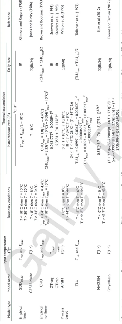
There are a variety of thermal functions in current crop models that capture the relationship between temperature and maize development. These functions vary in a number of ways, including parameter values, the quantity and quality of the data from which they were formulated, the complexity of the algorithm used to capture the relationship, and the manner in which the algorithms were derived (i.e., empirical or process based) (Table 1). The relationship between temperature and maize development can be derived either empirically or through a process-based methodology. For the purposes of this study, empirically derived functions are defined as those that are formulated and parameterized utilizing the same measured phenomenon as the phenomenon to be predicted (e.g., time from planting to anthesis). Thermal functions derived through process-based methodology are defined as those functions that are parameterized and derived utilizing information at a lower level of organization than the phenomenon that is to be predicted (e.g., enzyme kinetics to predict the time from planting to anthesis). The thermal functions studied here are grouped into three function types that represent simple linear empirical relationships (Gilmore and Rogers, 1958; Jones and Kiniry, 1986), more complex empirical nonlinear relationships (Brown, 1969; Stewart et al., 1998), and functions based on process-based relationships between temperature and biochemical or organ-level responses (Tollenaar et al., 1979; Kim et al., 2012; Parent and Tardieu, 2012). Differences in cardinal temperatures, as well as the relative rates of development within specific temperature ranges, are seen across the thermal functions studied (Table 1).

Despite the importance of thermal functions in the prediction of crop developmental stages and the variation in the currently utilized thermal functions, there is no clear indication of the relative precision of these functions in simulating crop developmental phases. Fundamental differences in the accuracy of these algorithms are largely unknown, partially due to the use of genotype coefficients that “fit” the genotype to a set of data. Therefore, the evaluation of thermal functions for the accurate simulation of maize

Ta bl e 1 . S um m ar y o f t he rm al f un ct io ns , i np ut t em pe ra tu re s ( da ily ), t em pe ra tu re b ou nd ar y c on di tio ns , a nd i ns ta nt an eo us a nd d ai ly r at es o f t he rm al a cc um ul at io n. T he g en er al t he rm al i nd ex ( G T I) m od el h as se pa ra te f un ct io ns f or t he p re -a nd p os t-flo w er in g p er io ds ( G T Iv eg a nd G T Ir ep , r es pe ct iv el y) . Model type Model name Input temperatur es (T )† Boundar y conditions Thermal accum ulation Ref er ence

Instantaneous rate (IR)

Dail y rate —————————————— °C d –1 —————————————— Empirical linear GDD 10,30 Tmin and Tmax T < 10 °C then T = 10 °C T > 30 °C then T = 30 °C (Tmin + Tmax )/2 – 10 °C IR Gilmor e and Rogers (1958) CERES-Maize T(1 h) T < 8 °C then T = 8 °C T > 34 °C then T = 34 °C T – 8 °C S (IR/24)

Jones and Kinir

y (1986) Empirical nonlinear CHU Tmin and Tmax Tmin < 4.4 °C then Tmin = 4.4 °C Tmax < 10 °C then Tmax = 10 °C CHU min = 1.8( Tmin – 4.4 °C) CHU max = 3.33( Tmax – 10 °C) – 0.084( Tmax – 10 °C) 2 (CHU max + CHU min )/2 Br

own and Bootsma (1993)

GTIv eg Tmean 0.043177 T 2 – 0.000894 T 3 IR Ste war t et al. (1998) GTIr ep Tmean 5.3581 + 0.011178 T 2 IR Ste war t et al. (1998) Pr ocess based APSIM T(3 h) T < 0 °C then T = 0 °C T > 44 °C then T = 44 °C 0 £ T < 18 °C: T 10/18 °C 18 £ T < 34 °C: T – 8 °C 34 £ T < 44 °C: 26 °C – ( T – 34 °C)2.6 S (IR/8) Wilson et al. (1995) TLU Tmin and Tmax T < 6 °C then T = 6 °C T > 44.8 °C then T = 44.8 °C TLU min = 0.0997 – 0.036 Tmin + 0.00362 Tmin 2 – 0.0000639 Tmin 3 TLU max = 0.0997 – 0.036 Tmax + 0.00362 Tmax 2 – 0.0000639 Tmax 3 (TLU max + TLU min )/2 Tollenaar et al. (1979) MAIZSIM T(1 h) T < 0 °C then T = 0 °C T > 43.7 °C then T = 43.7 °C 0.53[(43.7 – T)/11.6)( T/32.1)] 2.767 S (IR/24) Kim et al. (2012) EnzymResp T(1 h) (T + 273)exp{–73900/[8.314( T + 273)]}/[1 + (exp{–73900/[8.314( T + 273)]})3.5[1 – ( T + 273)/306.4)]51,559,240,052 S (IR/24) Par ent and Tar dieu (2012) † Tmin , d ai ly m in im um t em pe ra tu re ; Tma x , d ai ly m ax im um t em pe ra tu re ; T (1 h ), e st im at ed f ro m d ai ly Tmin a nd Tma x u si ng s in e-w av e t em pe ra tu re d is tr ib ut io n d ur in g a 2 4-h p er io d ( e. g. , T ol le na ar e t a l., 1 97 9) ; Tme an , d ai ly m ea n t em pe ra tu re ; T( 3 h ), e st im at ed f ro m r an ge f ra ct io ns t ha t d es cr ib e a s in e w av e.

Galley Proofs

development (while limiting potential biases imposed by the use of genotype coefficients) is an important inquiry.

In assessing the impact of climate change on crop productivity, assumptions are generally made about the hybrids adapted for a region or the date on which the hybrid was probably planted. In some applications of crop models, such as gridded models, instead of specific hybrids an “average” hybrid is used to capture the average response of hybrids adapted to the geographic region. To indicate the geographic region of adaptation, commercial hybrids are grouped by comparative relative maturity (Lauer, 1998), or simply relative maturity (RM). The determination of the developmental response of RM groups is therefore of value to modelers to simulate the “average” response of hybrids adapted to specific geographies. Variation in the precision of the thermal functions for different RM groups may indicate that some thermal functions are better able to capture the temperature variation extent in the geographies to which the RM groups are adapted or, alternatively, that RM group hybrids have different temperature responses. Therefore the relationship between RM groups and thermal function precision is an important consideration. An early vs. a delayed planting date may also impact the precision of thermal function in much the same way as RM group, again calling for consideration of how the precision of thermal functions may vary by the temperature variations that can result as a consequence of a change in planting date.

The overall goal of this study was to bring together researchers to evaluate a number of thermal functions for their ability to predict maize phenology across a range of source data that vary in the number of hybrids, geographies, and environmental conditions tested. The specific objectives of this study were (i) to assess the effect of source data on the ability to differentiate among thermal functions, (ii) to quantify the relative precision of eight thermal functions in predicting maize phenological development, and (iii) to attribute the precision of thermal functions to its response across various temperature ranges.

MATERIALS AND METHODS Thermal Functions

Eight thermal functions were selected for evaluation and classified according to their derivation type (i.e., empirical or process based) and thermal response. An empirical function is defined herein as a function for which the level of organization of its derivation and parameterization is the same as that of its outcome, e.g., the planting to anthesis interval of a field-grown maize canopy. In contrast, a process-based function is defined as a function that is derived and parameterized at a lower level of organization than that of its outcome, e.g., the derivation and parameterization of a function at the enzyme-kinetics level, whereas the outcome of the function is the planting to anthesis interval of a field-grown maize canopy. For the purposes of this study, the APSIM, TLU, MAIZSIM, and EnzymResp functions (defined below) were classified as process-based functions, and the GDD_10,30, CERES-Maize, CHU, and GTI functions (defined below) were classified as empirical functions. The empirical functions were subdivided into “linear” (GDD_10,30 and CERES-Maize) and “nonlinear” (CHU and GTI) functions, based on their temperature response at a constant temperature during a 24-h period. The thermal functions evaluated in this study are summarized in Table 1 and defined as follows:

1. GDD_10,30: Growing degree days (GDD) with a “base” temperature of 10°C and an “optimum” temperature at 30°C is a thermal function was developed by Gilmore and Rogers (1958) using 10 hybrids and 10 inbred lines grown at College Station, TX, at five planting dates in 1956. They calculated heat unit accumulation by subtracting 10°C from the daily minimum and maximum temperatures before cal-culating daily means, using six combinations of base (none or 10°C) and optimum (none, 30, or 32.2°C) temperatures. The method with the highest precision in their study was the classic 10/30°C cutoff method.

2. CERES-Maize (GDD_8,34): The CERES-Maize model uti-lizes GDD_8,34, with temperatures at hourly time steps esti-mated from the minimum and maximum temperatures. The GDD_8,34 is a linear function similar to GDD_10,30, but with base and optimum temperatures of 8 and 34°C, respectively. The original thermal function for CERES-Maize described by Jones and Kiniry (1986) used eight 3-h, third-order poly-nomial interpolations, but in the current version, thermal accumulation is calculated from temperatures during 24 1-h periods (J.T. Ritchie, personal communication, 1998), which are estimated using a sine wave between the minimum and the maximum daily temperatures (cf., Tollenaar et al., 1979). The Hybrid-Maize (Yang et al., 2006) and IXIM (Lizaso et al., 2011) models also use GDD_8,34, with eight 3-h and 24 1-h temperatures, respectively, estimated from minimum and maximum temperatures.

3. APSIM: The APSIM model uses a single multilinear func-tion for thermal accumulafunc-tion that reflects the biological response of development across the 0 to 44°C range in tem-peratures encountered in most environments in which maize is cultivated (Wilson et al., 1995). This temperature-response function has 0°C minimum, 34°C optimum, and 44°C ceiling temperatures. Daily thermal accumulation was calcu-lated from eight 3-h, third-order polynomial interpolations between the minimum and maximum daily temperatures. 4. Thermal leaf units (TLU). Analogous to accumulated

grow-ing degrees days in GDD_10,30 (°C d), TLU is accumulated thermal leaf units (L, leaf tips) by conversion of temperature to leaf (tip) units through the temperature-dependent rate of leaf appearance (L °C–1 d–1 ´ °C d = L), where the rate of leaf appearance (RLA) is the inverse of the phylochron. The relationship between the rate of leaf-tip appearance and temperature (Tollenaar et al., 1979) represents a biologically meaningful temperature response. This response is similar to other growth and development processes in maize such as seedling growth (Lehenbauer, 1914), radical elongation (Blacklow, 1972), and leaf elongation (Parent and Tardieu, 2012). The temperature-compensated rate of leaf-tip appear-ance is fairly constant until the emergence of the topmost leaf (Tollenaar et al., 1979, 1984). The number of visible leaf tips per plant is assumed to be equal to the accumulated TLU at any time between planting and the appearance of the topmost leaf if the rate of leaf appearance is influenced by temperature only. Based on this assumption, TLU accu-mulation between planting and anthesis is equal to the total leaf number plus the TLU accumulation during the interval between the appearance of the topmost leaf and anthesis. Leaf-ligulae appearance has also been used to quantify (e.g.,

Warrington and Kanemasu, 1983a) and to model (e.g., Parent et al., 2010) the rate of leaf appearance and maize de-velopment, among others, because of the wide use of V stages (Abendroth et al., 2011) to describe phenological develop-ment in maize. In contrast to the temperature-compensated rate of leaf-tip appearance, the temperature-compensated rate of leaf-ligule appearance varies widely for the planting to flowering interval. The ratio of the rate of leaf-tip appearance to the rate of leaf-ligule appearance is >1 during the first eight to 12 leaves, and it is <1 during the second half of the pre-silking period (Muldoon et al., 1984). The variability of the temperature-compensated rate of leaf-ligule appearance across the pre-silking phase diminishes its suitability for use in modeling the rate of maize development. Analogous to ac-cumulated growing degrees days in GDD_10,30 (°C d), TLU, (L °C–1 d–1 ´ °C d = L) are accumulated by the conversion of temperature to leaf tips through the RLA function. 5. MAIZSIM (b function): A b function was introduced by

Yin et al. (1995) that described the temperature response of crop development. This function describes a smooth non-symmetric response to temperature using five param-eters: three cardinal temperatures (the base temperature [T_base], the optimum temperature [T_opt], and the maxi-mum temperature [T_ceil]), a parameter for the maximum rate of development at T_opt (R_max), and a parameter that describes the curvature of the relationship. All parameters except the parameter that describes the curvature are bio-logically meaningful. Yan and Hunt (1999) simplified the Yin et al. (1995) function by eliminating the variable de-scribing the shape of the curve and by setting T_base to zero, resulting in the following equation with three parameters:

( )

= - æçç_ç ö÷÷_÷÷ ç ÷ - _{è ø} -opt ceil max

ceil opt opt ceil opt

T

T T T

R T R

T T T T T [1]

where R(T) is the rate of development as a function of

temperature. Yan and Hunt (1999) showed that this simplified b function was highly predictive when model parameters that were estimated from six constant tempera-tures were used to predict the rates of 16 varying day–night temperature regimes in the Tollenaar et al. (1979) data set. The MAIZSIM model (Kim et al., 2012) uses Eq. [1] for predicting the leaf appearance rate and assigned the follow-ing parameter values: T_opt = 31.2°C, T_ceil = 43.7°C, and

R_max = 0.53 d–1_.

6. Enzymatic response (EnzymResp): Using an equation for describing the temperature response of enzyme activities (Johnson et al., 1942), Parent et al. (2010) showed that processes linked to plant growth and development showed coordinated temperature responses and followed common laws within a plant species. Interestingly, they showed that there was no coordination of temperature responses linked to plant metabolism and leaf photosynthesis. In a meta-analysis, Parent and Tardieu (2012) utilized an equation to show a common response among maize genotypes from high-latitude, temperate, and tropical regions across a wide range in temperatures: ( ) æ _ö÷ ç _÷ ç ÷ çè ø a -æ _ö÷ ç ÷ ç ÷ çè ø -D = é ù +_êë -D _úû 1 T0 exp ( ) 1 exp A T A AT H RT R T H RT [2]

The function has two parameters: T₀ = 306.4°K ( = 33.3°C) and a = 3.5 (Parent and Tardieu, 2012). The parameter DH_A = 73900 J mol–1 _{is deduced from the other two. and} A is a size factor without units (51,559,240,052).

7. Crop heat units (CHU): Crop heat units have been used in Canada to account for temperature effects on phenology in maize since the mid-1960s. Crop heat units are estimated using separate night and day temperature functions (Table 1). The former is a linear function with a minimum of 4.4°C and the latter is a quadratic function with a minimum at 10°C and an optimum near 30°C (Brown, 1969). The quadratic function was developed by Brown (1960) from data collected on soybean [Glycine max (L.) Merr.] grown in

environment-controlled studies (Van Schaik and Probst, 1958).

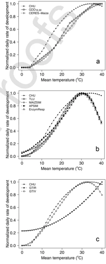
8. General thermal index (GTI): The GTI model is based on a large data set of maize hybrids grown during 4 yr at 19 loca-tions across a 9°interval in latitude across the North American Corn Belt, in which the durations from planting to silking and from silking to maturity were related to air temperature (Stewart et al., 1998). The GTI model is unique in that (i) it consists of two polynomial responses to temperature, one for the period from planting to silking and one for the period from silking to maturity, and (ii) the temperature response during the post-silking period was flat relative to that during the pre-silking period, particularly for temperatures <20°C (cf., Stewart et al., 1998, Fig. 2 and 5). Although the rela-tive insensitivity of the duration of the grain-filling period in maize to temperature has been reported previously (Shaw and Thom, 1951; Brown, 1977), none of the current thermal mod-els other than GTI account for differences in the temperature response between the pre- and post-flowering periods. Thermal functions can have a range of responses across temperatures and, consequently, the precision of the thermal functions will probably be related to their differential response across the temperature ranges to which they are exposed. Most figures of thermal functions in the literature graph the developmental response against a specific temperature value, which is useful for evaluating the function at the hour when the plant experienced the specific temperature. However, due to the diurnal range in temperatures to which plants are exposed daily, an hour snap shot is a limited perspective of the plant’s daily developmental response. Given that a location’s diurnal temperature variation is relatively stable, the response of thermal functions for a given diurnal range can be computed and graphed against a range of mean temperatures. To better capture how the thermal functions in this study respond to daily ambient conditions, the response of the thermal functions to mean temperature in the 0 to 45°C range was calculated assuming a diurnal temperature range of 12°C (i.e., the difference between T_max and T_min values). The 12°C diurnal temperature range value was selected because this was the approximate mean diurnal temperature range in the data sets utilized in the current study. To facilitate a comparison of the relative response, each function was normalized for the rate at its optimum temperature (Fig. 1).

Data Sources and Analyses

The precision of the thermal functions was evaluated using data from three different sources:

1. North America: Data were collected in field trials performed by Monsanto Co. that resulted in two different data sets. First, data were collected in trials that were performed from 2007 to 2011 at 43 locations across the North American Corn Belt. A total of 118 commercial DeKalb maize hybrids were tested that ranged from 76 to 119 RM. The hybrids were grown in their area of adaptation, and the number of locations in each of five RM classes was 13 for RM 76 to 85, 27 for RM 86 to 95, 26 for RM 96 to 105, 28 for RM 106 to 115, and 14 for RM 116 to 119 (i.e., the total number of locations is >43 because hybrids of more than one RM class were tested in several locations). The number of hybrids and locations tested varied each year. The data set consisted of 1375 combinations of hybrids ´ locations ´ years. Dates of planting and 50% anthesis were measured in this data set. The second data set was collected in trials that were performed from 2007 to 2012 at a location near DeKalb, IL. This location was not included in the 43-location North American data set. At this location, dates of black layer formation (i.e., physiological maturity), anthesis, and silking were recorded on 3129 hybrids ´ years, and the hybrids tested included all 118 hybrids grown at the other 43 loca-tions. The hybrids in this data set ranged in RM from 76 to 119. At all locations, maize hybrids were grown in 6.1-m-long, four-row plots using standard agronomic practices. 2. Indiana–Ohio: This data set consisted of 108 entries. Details

of this study have been previously reported by Nielsen et al. (2002). In short, three Pioneer maize hybrids (CRM 106, 111, and 115) were grown at three planting dates, ranging from 22 April to 17 June, each at four locations in Ohio and Indiana from 1991 to 1994. Note that Pioneer uses CRM (comparative relative maturity) to designate hybrid RM and that hybrid RM ratings may vary somewhat among differ-ent seed companies (Lauer, 1998). Dates of 50% silking and 50% black layer were recorded.

3. Argentina: This data set consists of information collected on various maize hybrids ranging from RM 92 and 127 that were grown between 1988 and 2013 near Balcarce, Argen-tina. Data included the results of a published study (Cirilo and Andrade, 1994a, 1994b) and several unpublished studies. Some of the studies had multiple planting dates that ranged from September to January. The experimental area was irrigated when deemed necessary. Dates of 50% silking and 50% black layer were recorded.

Weather data were collected for each location-year in the three data sets. Records of daily maximum and minimum air temperatures were obtained either from the National Climate Data Center (U.S. weather stations, http://www.ncdc.noaa. gov/cdo-web/search) or the Government of Canada Climate Service (Canadian weather stations, http://climate.weather. gc.ca/index_e.html#access) for the location-years in the North American and Indiana–Ohio data sets. All weather service stations were, on average, within 20 km of the experimental site.

Field data were analyzed for the pre-flowering and post-flowering periods. The pre-post-flowering period was defined as the period from the first day after planting until, and including,

Fig. 1. Relationships between mean daily temperatures with a 12°C diurnal range normalized for rate of development at the optimum temperature

specific to each function: (a) growing degree days (GDD_10,30),

CERES-Maize, and crop heat units (CHU) functions, (b) APSIM, thermal leaf units (TLU), MAIZSIM, EnzymResp, and CHU functions, and (c) general thermal index (GTI) during the preflowering period (GTIV), GTI during the post-flowering period (GTIR), and CHU functions.

anthesis (i.e., the first day at which ³50% of plants shed pollen) or silking (i.e., the first day at which silks had emerged from the topmost ear shoot in ³50% of plants), and the post-silking period was defined as the first day after silking until, and including, black layer (the first day on which 50% of plants have grain with a black layer in the center portion of the ear). Whenever possible, the planting to anthesis interval rather than the planting to silking interval was analyzed because the anthesis to silking interval is highly affected by abiotic stresses (Edmeades et al., 2000) and, consequently, the use of the silking date will introduce another potential unaccounted source of variability in the data.

Daily thermal accumulation was estimated using the daily mean temperature (GTI), minimum and maximum temperatures (GDD_10,30 and CHU), 1-h temperatures (CERES-Maize, TLU, MAIZSIM, and EnzymResp), and 3-h temperatures (APSIM). The 1-h temperatures were estimated using a sine wave between the minimum and the maximum daily temperature (e.g., Tollenaar et al., 1979). The 3-h temperatures in the APSIM function were estimated using range fractions for each of the eight time periods within a 24-h day that describe a sine wave.

The CV (coefficient of variability) was used to quantify the precision of the thermal functions. The mean thermal accumulation (and days), standard deviation, and CV were calculated from all observations (i.e., hybrid-location-year) within an RM class for the North American data set and within a planting date for the Indiana–Ohio and Argentinean data sets for the planting to anthesis (or silking) interval and the silking to physiological maturity interval. Statistical analyses of the CVs were performed using the Glimmix procedure for generalized linear modeling assuming a log link and g distribution in SAS, Version 9.3, where RM classes or planting dates were replications for the statistical comparisons among thermal functions, and thermal functions were replications for the statistical comparisons among either RM classes or planting dates.

Differences in the precision of the thermal functions across RM groups may be due to genetic or environmental factors associated with the regions to which the RM groups are adapted. One method for deconstructing these factors is to identify differences in cardinal temperatures among RM classes. Since the MAIZSIM function explicitly quantifies T_opt and T_ceil values, optimization of this function for each of the five RM classes can identify these cardinal temperatures of each RM class. The optimization procedure of the b function was performed by varying the values of T_opt and T_ceil (keeping T_base unchanged at 0°C) and selection based on the lowest CV. The optimization of the b function was done using the optimum function of the R statistical language (R Development Core Team, 2013) with the Nelder–Mead algorithm for both entries in each of the five RM classes of the 43-location North American data set and for all RM classes combined (b_OPT). This is a general purpose routine for function error minimization. Several of the minimization calculations were run for two different starting values, and the results were identical in the two cases. This exercise confirmed that the algorithm was converging to a global rather than to a local optimum.

In addition, for each of the five RM class in the 43-location North America data set, the hybrid-location-years of the data set were subdivided equally into three groups representing 33% low, 33% medium, and 33% high means of daily minimum

temperature and of daily maximum temperature, resulting in 15 mean-minimum and 15 mean-maximum temperature groups (i.e., 5 RM classes ´ 3 groups within each RM class). This analysis is informative of thermal function sensitivity variation by temperature. The thermal functions tested vary in T_base, T_opt, and T_max values. Differences in cardinal temperature may render some thermal functions more sensitive to specific temperatures than others, thus impacting their relative precision in simulating development.

RESULTS AND DISCUSSION Impact of Data Source on Thermal

Function Evaluation

Data source is an important variable when evaluating the precision of thermal functions. The data sets evaluated in this study each had limitations. The Indiana–Ohio data set was comprised of a multilocation, multiyear study with orthogonal treatments, but contained only a relatively small number of hybrids and environments (i.e., location-years). In contrast, the North American data sets consisted of a large number of hybrids and environments, but the treatments were not orthogonal. Different hybrids were grown in each location-year, resulting in a different number of observations for each RM class in the 43-location data set (Tables 2 and 3). In addition, the silking to black layer interval was evaluated only at a single geographic location near DeKalb, IL, for multiple years (Table 3). The Argentinean data set was not orthogonal and contained a relatively small number of environments (years).

Empirical nonlinear functions were more precise than either empirical linear or process-based functions in the North American and Indiana–Ohio data sets, but the precision of the thermal functions did not differ in the Argentinean data set (Tables 2–6). Differences among thermal functions and calendar days were generally smaller in the Indiana–Ohio than the North American data set. The precision of the thermal functions for the planting to anthesis phase in the North American data set were calendar days < empirical linear < process based < empirical nonlinear, whereas in the Indiana–Ohio data set they were calendar days < empirical linear = process based < empirical nonlinear. In the Argentinean data set, calendar days were less precise than the thermal functions, but the thermal functions could not be differentiated. Therefore, large data sets have improved ability to differentiate thermal function performance, even when they may have limitations such as lack of orthogonality. Ideally, large and orthogonal data sets would be preferred.

Relative Precision of Thermal Functions

Within the large data sets that allowed the greatest differentiation among the thermal functions, the empirical nonlinear functions proved to be more precise than the other functions tested (Tables 2–6). Thermal functions were generally more precise than calendar days, although differences were smaller during the period between silking and black layer than during the planting to anthesis interval. The precision of the thermal functions for both the pre-flowering and post-flowering period in the North American data set was empirical linear < process based < empirical nonlinear (Table 6). The CHU and GTI functions were the most precise for the prediction of both the pre-anthesis and post-silking phases in the North American

data set (Tables 2 and 3). In the Indiana–Ohio data set, the GTI function was the only thermal function that was more precise than calendar days for the silking to black layer period (Table 4). The post-flowering GTI thermal function had a very different thermal response than any other thermal function tested (Fig. 1). The higher precision of GTI for the post-flowering period was associated with a relatively small difference in thermal accumulation from silking to maturity between the early and late planting dates for GTI. Nielsen et al. (2002) showed a 17% difference in GDD_10,30 accumulation during the post-flowering period between early and late planting, whereas the difference

in GTI accumulation was only 5% (data not shown). The mean minimum daily temperatures during the silking to black layer interval decreased from 14.3 to 10.7°C for the early and late planting dates, respectively.

Relationship between Temperature Response and Precision of Thermal Functions

The precision of the thermal functions is associated with their response across a wide range of temperatures. One means of understanding the precision of thermal functions is to compare their normalized response across a range of temperatures in

Table 2. Coefficients of variation of the number of days and thermal accumulation during the planting to anthesis interval determined by eight func-tions for commercial hybrids across five relative maturity (RM) groups grown at 43 locafunc-tions in the Corn Belt from 2007 to 2011 (North American data set). The number of observations (n) is the sum of all hybrids grown in each location-year for a RM class.

RM n

Coefficient of variation

Days GDD_10,30 CERES MAIZSIM TLU EnzymResp APSIM GTI CHU

—————————————————————————– % —————————————————————————– 76–85 121 10.3 9.5 9.3 9.0 8.4 9.0 7.8 7.6 7.0 86–95 204 9.9 9.7 9.5 9.2 8.5 9.2 7.7 7.6 6.8 96–105 342 9.3 6.4 6.5 6.2 6.0 6.3 6.0 5.7 5.6 106–115 560 10.4 6.4 6.9 6.0 5.3 6.2 5.4 4.7 4.5 116–122 148 10.3 6.3 6.9 5.9 5.3 6.0 5.2 4.5 4.6 Mean 10.1 e† 7.7 d 7.8 d 7.3 cd 6.7 c 7.3 d 6.4 bc 6.0 ab 5.7 a All 1375 10.7 10.1 10.2 9.5 8.7 9.6 7.9 7.5 6.7

† Means within a row followed by the same letter are not significantly different at the 0.05 level of probability.

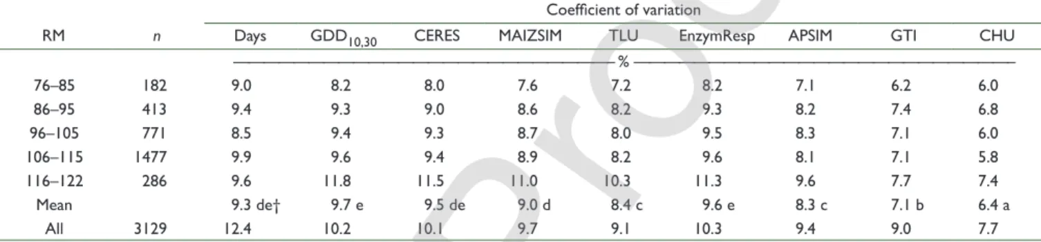
Table 3. Coefficients of variation of the number of days and thermal accumulation during the silking to black layer interval determined by eight thermal functions for commercial hybrids across five relative maturity (RM) classes grown at a single location in the U.S. Corn Belt from 2007 to 2012 (North American data set). The number of observations (n) is the sum of all hybrids grown in each location-year for a RM class.

RM n

Coefficient of variation

Days GDD_10,30 CERES MAIZSIM TLU EnzymResp APSIM GTI CHU

—————————————————————————– % —————————————————————————– 76–85 182 9.0 8.2 8.0 7.6 7.2 8.2 7.1 6.2 6.0 86–95 413 9.4 9.3 9.0 8.6 8.2 9.3 8.2 7.4 6.8 96–105 771 8.5 9.4 9.3 8.7 8.0 9.5 8.3 7.1 6.0 106–115 1477 9.9 9.6 9.4 8.9 8.2 9.6 8.1 7.1 5.8 116–122 286 9.6 11.8 11.5 11.0 10.3 11.3 9.6 7.7 7.4 Mean 9.3 de† 9.7 e 9.5 de 9.0 d 8.4 c 9.6 e 8.3 c 7.1 b 6.4 a All 3129 12.4 10.2 10.1 9.7 9.1 10.3 9.4 9.0 7.7

† Means within a row followed by the same letter are not significantly different at the 0.05 level of probability.

Table 4. Coefficients of variation of the number of days and thermal accumulation during the planting to silking and silking to black layer intervals de-termined by eight thermal functions for three maize hybrids planted at three dates from April to June during 1990 to 1994 at four locations in Ohio and Indiana (Nielsen et al., 2002); the total number of observations is 108. Data were analyzed both separately for the early, medium, and late planting dates and together for all planting dates.

Planting date

Coefficient of variation

Days GDD_10,30 CERES MAIZSIM TLU EnzymResp APSIM GTI CHU

—————————————————————————– % —————————————————————————– Planting to silking

Early 11.6 4.4 5.2 4.7 3.6 4.5 5.9 4.4 3.5

Medium 9.1 4.7 5.4 4.9 3.9 4.9 6.1 4.5 3.8

Late 5.6 5.7 6.4 6.1 5.2 6.1 7.2 5.7 4.7

Mean 8.8e† 4.9abc 5.7cd 5.3bcd 4.2ab 5.2bcd 6.4d 4.8abc 4.0a

All 12.9 5.2 5.8 5.5 4.7 5.5 7.0 5.4 5.0

Silking to black layer

Early 9.5 8.4 9.2 9.0 7.9 8.7 10.1 6.8 8.0

Medium 11.5 9.0 10.2 10.0 8.6 9.4 11.0 7.6 8.9

Late 8.6 11.3 12.7 12.5 10.7 11.8 14.0 8.6 10.5

Mean 9.9bc 9.6bc 10.7cd 10.5cd 9.0b 10.0bc 11.7d 7.7a 9.1b

All 10.3 11.8 13.1 12.8 11.0 12.0 12.8 7.9 10.5

† Means within row followed by the same letter are not significantly different at 0.05 level of probability.

relation to that of CHU, which has been shown to be more precise in the North American data set (Fig. 1). The results of the normalized responses to mean temperatures (based on a 12°C diurnal range) show that: (i) the empirical functions (GDD_10,30 and CERES) have a linear-like response between mean temperatures of 4 and 36°C (Fig. 1a) (the generally depicted temperature response of GDD_10,30 in the literature is a straight line between 10 and 30°C, but this is true only when there is no diurnal temperature variation or if the maximum and minimum daily temperatures are >10°C and <30°C); (ii) the process-based functions (TLU, APSIM, MAIZSIM, and EnzymResp) have a temperature response similar to each other in the 15 to 45°C temperature range, with small differences in the lower temperature range (Fig. 1b); and (iii) the nonlinear empirical functions are similar to each other across 0 to 30°C for the pre-silking phase (Fig. 1c). The post-silking GTI function has a very different temperature response that is relatively insensitive at temperatures <23°C (Stewart et al., 1998).

In this study, the nonlinear empirical functions were the most precise group of thermal functions tested, and differences in precision were associated with response in the 10 to 26°C mean diurnal temperature range (Fig. 1). Unlike linear empirical functions, the shape of process-based functions and the nonlinear

empirical function are similar (Fig. 1). These two groups of thermal functions varied somewhat in their base temperatures (Fig. 1b and 1c), but there was no consistent relationship between the base temperatures and the precision of the function (Tables 2–5). All three groups differ in the supra-optimal temperature range. However, differences in precision cannot be attributed to the developmental responses in the supra-optimal temperature range because none of the data sets used in this study contained mean daily temperatures >30°C. Differences in precision among thermal functions were associated with their relative temperature response in the 10 to 26°C mean diurnal temperature range (Fig. 1). The CHU function had higher developmental rates across the 10 to 26°C range and was the most precise in predicting phenology. At 20°C, for instance, the rate of development of CHU is 21% greater than that of TLU, and the rate of development of TLU is 21% greater than that of GDD_10,30 (Fig. 1), while precision of the three functions in the North American data sets was in the order CHU > TLU > GDD_10,30 (Tables 2 and 3). Thermal functions with higher normalized developmental rates across a wide range of temperatures (e.g., nonlinear empirical functions) have lower temperature sensitivity.

The precision of the thermal functions varied with RM class in the North American data set, and the variation in precision

Table 5. Coefficients of variation of number of days and thermal accumulation by eight functions during the planting-silking and silking-black layer in-tervals of maize hybrids planted from September to January between 1989 and 2012 at locations near Balcarce (Argentina). Data were analyzed both separately for four planting-date periods and together for all planting dates. The number of observations (n) is the sum of all hybrids grown in each location-year for a RM class.

Planting date n

Coefficient of variation

Days GDD_10,30 CERES MAIZSIM TLU EnzymResp APSIM GTI CHU

—————————————————————————– % —————————————————————————– Planting to silking Sept. 6 5.4 8.2 7.8 7.7 7.6 7.6 6.7 7.0 6.9 Oct. 41 6.7 6.2 6.5 6.2 5.6 6.4 6.5 6.3 5.5 Nov. 13 9.0 8.5 8.7 8.5 8.3 8.7 8.6 8.4 8.1 Dec.–Jan. 16 12.5 9.9 10.0 9.9 10.0 9.9 10.2 10.2 10.8 Mean 8.4 a† 8.2 a 8.2 a 8.1 a 7.9 a 8.2 a 8.0 a 8.0 a 7.8 a All 76 18.5 8.8 9.1 9.0 9.0 9.2 10.3 10.1 10.7

Silking to black layer

Sept. 6 6.7 6.0 5.0 5.4 5.7 5.6 5.1 5.4 5.4 Oct. 41 12.5 12.6 13.0 12.7 12.1 12.8 12.9 12.7 11.9 Nov. 13 18.7 11.0 10.3 10.8 11.9 11.0 11.8 13.6 13.3 Dec.–Jan. 16 11.0 8.6 8.5 8.4 8.4 8.1 7.6 8.2 8.7 Mean 12.2 b 9.6 a 9.2 a 9.3 a 9.5 a 9.4 a 9.4 a 10.0 a 9.9 a All 76 13.0 17.0 17.5 16.8 15.7 17.0 15.7 14.1 14.0

† Means within row followed by the same letter are not significantly different at 0.05 level of probability.

Table 6. Mean coefficients of variation of calendar days and thermal accumulation determined by empirical-linear functions (GDD_10,30 and

CERES-Maize), process-based functions (APSIM, MAIZSIM, EnzymResp, and TLU), and empirical-nonlinear functions (GTI and CHU) during the planting to anthesis or silking and the silking to black layer intervals in the 43-location, 5-yr and the one-location, 6-yr North American data sets (Tables 2 and 3), the Indiana–Ohio data set (Table 4), and the Argentinean data set (Table 5).

Phase of development Data set

Coefficient of variation Calendar days

Thermal function

Empirical linear Process-based Empirical nonlinear ——————————————————— % ——————————————————— Planting to anthesis or silking North America 10.1 d† 7.7 c 6.9 b 5.9 a

Indiana–Ohio 8.8 c 5.3 b 5.3 b 4.4 a

Argentina 8.4 8.2 8.0 7.9

Silking to black layer North America 9.3 c 9.6 c 8.8 b 6.8 a

Indiana–Ohio 9.9 ab 10.1 b 10.3 b 8.4 a

Argentina 12.2 b 9.4 a 9.4 a 9.8 a

† Means within a row followed by the same letter are not significantly different at the 0.05 level of probability.

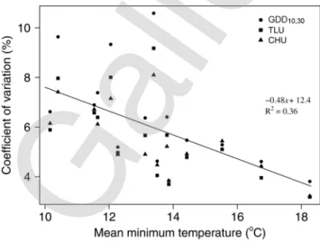
was associated with air temperature. The precision of the thermal functions increased from low- to high-RM classes during the planting to anthesis interval (Table 7) in the 43-location North America data set. This relationship between RM class and thermal function precision could be due to either genetics or environment. The association with genetics was dismissed because, when all RM hybrids were grown at a single location (i.e., the DeKalb, IL location), the trend in RM precision was no longer observed, i.e., there was either an opposite trend during the silking to black layer period (Table 7) or no trend during the planting to anthesis interval (data not shown). The effects of temperature on the relative precision of thermal methods across the RM groups in the North American data set was examined in more detail by subdividing each of the five RM groups of environments into three mean-minimum-temperature environments (Fig. 2). In this analysis, the change in CV of each thermal function across the 15 temperature–RM groups was –0.55% °C–1 _{for GDD}

10,30, –0.49% °C–1 for TLU, and

–0.41% °C–1 _{for CHU, but these slopes were not significantly}

different (data not shown). The CVs in some of the temperature environments deviated substantially from the regression (Fig. 2), and variation among the three thermal functions within these environments was small when the deviation from the regression was negative (e.g., the 10.2, 12.3, and 13.9°C environments) and

was large when the deviation from the regression was positive (e.g., the 10.4, 12.0, and 13.4°C environments).

When the b function was optimized for five RM groups, the values of T_opt and T_ceil of the early RM classes (Table 8) were much lower than reported values from controlled-environment studies (e.g., Parent et al., 2010; Sanchez et al., 2014). The low

T_opt and T_ceil values were probably not due to genetic differences among RM groups. Low T_opt (21.2 and 22.3°C) has been reported for the temperature-dependent duration of the period from sowing to tassel initiation for two highland tropical inbred lines in controlled-environment studies performed by Ellis et al. (1992) and reported by Yin et al. (1995), but neither the results of Tollenaar et al. (1979), which included North American hybrids of <85 RM, nor the results of Parent and Tardieu (2012), which included very early European hybrids and inbred lines, showed T_opt and T_ceil values that were lower than those reported in studies of temperature-dependent rates of growth and development in maize (cf., Parent and Tardieu, 2012).

The relatively high precision of temperature-insensitive functions, the decline in CV with increase in temperature among RM groups, and low cardinal temperatures in the optimized b function of early RM groups all support the contention that maize phenology is influenced by factors other than air temperature per se. Factors other than air temperature that can influence phenology include soil and apex temperature (Vinocur and Ritchie, 2001), photoperiod (e.g., Kiniry et al., 1983; Tollenaar and Hunter, 1983; Warrington and Kanemasu, 1983b), incident solar radiation (Birch et al., 1998, Tollenaar,

Table 7. Mean coefficient of variations (CV) of thermal accumulation determined by eight functions during the planting to anthesis and silking to black layer intervals, and mean daily minimum and maximum temperatures of locations for five relative maturity (RM) groups. The planting-to-anthesis interval comprised observations across 43 Corn-Belt locations during 2007 to 2011 (Table 1) and the silking to black layer interval comprised > 3100 observations at one Corn-Belt location from 2007 to 2012 (North American data sets).

RM

Planting to anthesis Silking to black layer CV

Daily temperature

CV

Daily temperature

Min. Max. Min. Max.

d % ——————— °C ——————— % ——————— °C ——————— 76–85 8.5 c† 11.7 23.1 7.3 a 17.1 28.4 86–95 8.5 c 12.1 23.9 8.4 b 16.9 27.9 96–105 6.1 b 13.0 25.4 8.3 b 16.6 27.7 106–115 5.7 a 14.3 26.3 8.3 b 15.6 26.7 116–122 5.6 a 15.7 27.5 10.1 c 15.1 26.3

† Means within a column followed by the same letter are not significantly different at the 0.05 level of probability.

Table 8. Coefficients of variation (CV) for the planting to anthesis in-terval of thermal functions that utilize different forms of the b function: the MAIZSIM b function, and different b functions modified to optimize CV by changing Topt and Tceil (within parentheses) within each of the five relative maturity (RM) classes. The optimization procedure of the b function was performed by varying the values of the optimum

tem-perature (T_opt) and the maximum temperature (T_ceil) (keeping T_base

unchanged at 0°C). Mean CVs of b_OPT and MAIZSIM are significantly

different at 0.05 level of probability.

RM Coefficient of variation bOPT MAIZSIM b d ————————— % ————————— 76–85 6.2 (23.0, 32.4)† 9.0 (32.1, 43.7) 86–95 6.3 (25.7, 39.6) 9.2 (32.1, 43.7) 96–105 5.4 (26.2, 35.9) 6.2 (32.1, 43.7) 106–115 4.3 (27.6, 37.8) 6.0 (32.1, 43.7) 116–122 4.3 (30.3, 44.9) 5.9 (32.1, 43.7) † Topt, Tceil (°C) in parentheses.

Fig. 2. Relationship between mean minimum temperature and CVs

of the growing degree day (GDD_10,30), thermal leaf units (TLU), and

crop heat units (CHU) functions for 12 environments (location-years). Environments were grouped into the 33% highest, 33% medium, and 33% lowest mean minimum temperature environments in each of the five relative maturity classes depicted in Table 7.

1999), and periods of severe stress (e.g., McCullough et al., 1994). For instance, apex temperature is influenced by plant transpiration and soil temperature before the eight-leaf-tip stage and the apex-air temperature differential appears to be greatest at low temperatures (Vinocur and Ritchie, 2001; Birch et al., 1998). The apex-air temperature differential may have played a role in the higher precision of less temperature-sensitive functions, the increase in precision with temperature among RM groups, and the low T_opt and T_ceil values for the early RM groups in the MAIZSIM optimization. The lower precision of process-based functions may be due to the fact that these data sets were generated under controlled-environment conditions where many of the factors other than air temperature were held constant and where the apex-air temperature differential may have been less than under field conditions.

Precision of Thermal Functions under Supra-Optimal Temperatures

Climate change will probably result in an increase in the number of days in the growing season with elevated temperatures, and therefore an accurate estimate of the impact of supra-optimal temperatures on maize phenology will be important in evaluating the impact of climate change on maize yield. The response to supra-optimal temperature differs substantially among the thermal functions (Fig. 1).The process-based thermal functions TLU, MAIZSIM, and EnzymResp are derived from data that includes supra-optimal temperatures. These functions were derived from controlled-environment studies during early phases of development that showed that the rate of development declines rapidly when temperatures are raised beyond the optimum temperature (Lehenbauer, 1914; Tollenaar et al., 1979; Warrington and Kanemasu, 1983a,b; Parent and Tardieu, 2012). In contrast, the rate of development remains constant beyond 36°C for empirical linear functions and declines moderately beyond the optimum temperature in nonlinear empirical functions that account for the whole life cycle (Fig. 1). Nonlinear empirical functions were derived based on data sets that contained either no or few supra-optimal temperatures (i.e., Van Schaik and Probst, 1958; Brown, 1960; Stewart et al., 1998), and the precision of these functions may be low for supra-optimal conditions. Hence, while data are limited on the supra-optimal range, we suggest that maize models that are used to assess the impact of climate change on crop productivity should utilize the developmental response to supra-optimal temperatures of process-based functions for the pre-flowering period. Even less is known about the developmental response to supra-optimal temperatures during the grain-filling period. The GTI and CHU functions performed best during the post-silking period in the data sets evaluated here (Tables 3 and 4), with mean temperatures <25°C. To the best of our knowledge, no information is available on the response of the grain-filling period to supra-optimal temperatures. Owing to the paucity of supra-optimal temperature data in the derivation or evaluation of empirical thermal functions, process-based functions appear to better represent the temperature response of maize development under supra-optimal temperatures. Overestimation of the rate of development under supra-optimal temperatures by empirical models will lead to a disproportionate reduction of the life cycle, and consequently, models that use empirical thermal functions will underpredict yield in climate-change scenarios.

CONCLUSIONS

The results of this study show that large data sets can improve the ability to differentiate among thermal functions that quantify the effect of temperature on maize phenology. The precision of nonlinear empirical functions, particularly CHU, is superior to that of both linear empirical functions, such as GDD_10,30, and process-based functions, such as the TLU function, in predicting maize phenology. The precision of thermal functions was associated with the temperature response across the 10 to 26°C temperature range rather than with the base and optimum cardinal temperatures or the supra-optimal temperature range. The higher precision of the CHU function is associated with its overall lower relative temperature sensitivity in the 10 to 26°C temperature range, which is probably due to factors other than air temperature that influence rate of development. The GTI function during the post-silking period has a low temperature sensitivity for temperatures <23°C (Fig. 1c), and this function was superior for the Indiana–Ohio data set. Because the nonlinear empirical functions were developed under conditions devoid of supra-optimal temperatures, and while we await for research addressing the response to temperature in that range, maize models that are used to assess the impact of climate change on crop productivity should utilize the developmental response of process-based functions to quantify the response of phenology to supra-optimal temperatures during the pre-flowering period.

REFERENCES

Abendroth, L.J., R.W. Elmore, M.J. Boyer, and S.K. Marlay. 2011. Corn growth and development. PMR 1009. Iowa State Univ. Ext., Ames.

Asseng, S., F. Ewert, C. Rosenzweig, J.W. Jones, J. L. Hatfield, A.C. Ruane, et al. 2013. Uncertainty in simulating wheat yields under climate change. Nature Clim. Change 3:827–832. doi:10.1038/nclimate1916

Birch, C.J., J. Vos, J. Kiniry, H.J. Bos, and A. Elings. 1998. Phyllochron responds to acclimation to temperature and irradiance in maize. Field Crops Res. 59:187–200. doi:10.1016/S0378-4290(98)00120-8

Blacklow, W.M. 1972. Influence of temperature on germination and elongation of the radicle and shoot of corn (Zea mays L.). Crop Sci. 12:647–650.

doi:10.2135/cropsci1972.0011183X001200050028x

Brown, D.M. 1960. Soybean ecology: I. Development–temperature relationships from controlled-environment studies. Agron. J. 52:493–496. doi:10.2134/ agronj1960.00021962005200090001x

Brown, D.M. 1969. Heat units for corn in southern Ontario. Ministry of Agric. and Food, Guelph, ON, Canada.

Brown, D.M. 1977. Response of maize to environmental temperatures: A review. In: W. Baier, editor, Proceedings of the WMO Symposium on Agrometeorology of the Maize (Corn) Crop, Ames, IA. 5–9 July 1976. World Meteorol. Organ., Geneva, Switzerland. p. 15–26.

Brown, D.M., and A. Bootsma. 1993.Crop heat units for corn and other warm season crops in Ontario. Ministry of Agriculture and Food, Guelph, ON, Canada.

Cirilo, A.G., and F.H. Andrade. 1994a. Sowing date and maize productivity: I. Crop growth and dry matter partitioning. Crop Sci. 34:1039–1043. doi:10.2135/cropsci1994.0011183X003400040037x

Cirilo, A.G., and F.H. Andrade. 1994b. Sowing date and maize productivity: II. Kernel number determination. Crop Sci. 34:1044–1046. doi:10.2135/cro psci1994.0011183X003400040038x

Edmeades, G.O., J. Bolaños, A. Elings, J.-M. Ribault, M. Bänziger, and M.E. Westgate. 2000. The role and regulation of the anthesis–silking interval in maize. In: M. Westgate and K. Boote, editors, Physiology and modeling kernel set in maize. CSSA Spec. Publ. 29. CSSA and ASA, Madison, WI. p. 43–73. doi:10.2135/cssaspecpub29.c4

Ellis, R.H., R.J. Summerfield, G.O. Edmeades, and E.H. Roberts. 1992. Photoperiod, leaf number, and interval from tassel initiation to emergence in diverse cultivars of maize. Crop Sci. 32:398–403.

Gilmore, E.C., and J.S. Rogers. 1958. Heat units as a method of measuring maturity in corn. Agron. J. 50:611–615. doi:10.2134/agronj1958.000219 62005000100014x

Intergovernmental Panel on Climate Change. 2007. Climate change 2007: Synthesis report. Contribution of Working Groups I, II, and III to the Fourth Assessment Report of the Intergovernmental Panel on Climate Change. IPCC, Geneva Switzerland. http://www.ipcc.ch/pdf/assessment-report/ar4/syr/ar4_syr.pdf.

Johnson, F.H., H. Eyring, and R.W. Williams. 1942. The nature of enzyme inhibitions in bacterial luminescence: Sulfanilamide, urethane, temperature and pressure. J. Cell. Comp. Physiol. 20:247–268. doi:10.1002/jcp.1030200302

Jones, C.A., and J.R. Kiniry. 1986. CERES-Maize: A simulation model of maize growth and development. Texas A&M Univ. Press, College Station, TX. Kim, S.-H., Y. Yang, D.J. Timlin, D.H. Fleisher, A. Dathe, V.R. Reddy,

and K. Staver. 2012. Modeling temperature responses of leaf growth, development, and biomass in maize with MAIZSIM. Agron. J. 104:1523– 1537. doi:10.2134/agronj2011.0321

Kiniry, J.R., J.T. Ritchie, R.L. Musser, E.P. Flint, and W.C. Iwig. 1983. The photoperiod sensitive interval in maize. Agron. J. 75:687–690. doi:10.2134/agronj1983.00021962007500040026x

Lauer, J. 1998. The Wisconsin comparative relative maturity (CRM) system for corn. Field Crops 28.31-21. Agron. Advice (December). http://corn. agronomy.wisc.edu/AA/A021.aspx.

Lehenbauer, P.A. 1914. Growth of maize seedlings in relation to temperature. Physiol. Res. 1:247–288.

Lizaso, J.I., K.J. Boote, J.W. Jones, C.H. Porter, L. Echarte, M.E. Westgate, and G. Sonohat. 2011. CSM-IXIM: A new maize simulation model for DSSAT Version 4.5. Agron. J. 103:766–779. doi:10.2134/agronj2010.0423 McCullough, D.E., Ph. Girardin, M. Mihajlovic, A. Aguilera, and M. Tollenaar.

1994. Influence of N supply on development and dry matter accumulation of an old and a new maize hybrid. Can. J. Plant Sci. 74:471–477. doi:10.4141/cjps94-087

Muldoon, J.F., T.B. Daynard, B. Van Duinen, and M. Tollenaar. 1984. Comparisons among rates of appearance of leaf tips, collars, and leaf area in maize (Zea mays L.). Maydica 29:109–120.

Nielsen, R.L., P.R. Thomison, G.A. Brown, A.L. Halter, J. Wells, and K.L. Wuethrich. 2002. Delayed planting effects on flowering and grain maturation of dent corn. Agron. J. 94:549–558. doi:10.2134/ agronj2002.5490

Parent, B., and F. Tardieu. 2012. Temperature responses of developmental processes have not been affected by breeding in different ecological areas for 17 crop species. New Phytol. 194:760–774. doi:10.1111/j.1469-8137.2012.04086.x

Parent, B., O. Turc, M. Gibon, M. Stitt, and F. Tardieu. 2010. Modelling temperature-compensated physiological rates, based on the co-ordination of responses to temperature of developmental processes. J. Exp. Bot. 61:2057–2069. doi:10.1093/jxb/erq003

R Development Core Team. 2013. R: A language and environment for statistical computing. R Found. Stat. Comput., Vienna, Austria.

Sanchez, B.A., A. Rasmussen, and J.P. Porter. 2014. Temperatures and the growth and development of maize and rice: A review. Global Change Biol. 20:408–417. doi:10.1111/gcb.12389

Shaw, R.H., and H.C.S. Thom. 1951. On the phenology of field corn, silking to maturity. Agron. J. 43:541–546. doi:10.2134/agronj1951.000219620043 00110004x

Stewart, D.W., L.M. Dwyer, and L.L. Carrigan. 1998. Phenological temperature response of maize. Agron. J. 90:73–79. doi:10.2134/agronj1998.0002196 2009000010014x

Tollenaar, M. 1999. Duration of the grain-filling period in maize is not affected by photoperiod and incident PPFD during the vegetative phase. Field Crops Res. 62:15–21. doi:10.1016/S0378-4290(98)00170-1

Tollenaar, M., T.B. Daynard, and R.B. Hunter. 1979. Effect of temperature on rate of leaf appearance and flowering date in maize. Crop Sci. 19:363–366. doi:10.2135/cropsci1979.0011183X001900030022x

Tollenaar, M., and R.B. Hunter. 1983. A photoperiod and temperature sensitive period for leaf number in maize. Crop Sci. 23:457–460. doi:10.2135/crops ci1983.0011183X002300030004x

Tollenaar, M., J.F. Muldoon, and T.B. Daynard. 1984. Differences in rate of leaf appearance among maize hybrids and phases of development. Can. J. Plant Sci. 64:759–763. doi:10.4141/cjps84-104

Van Schaik, P.H., and A.H. Probst. 1958. Effects of some environmental factors on flower production and reproductive efficiency in soybeans. Agron. J. 50:192–197. doi:10.2134/agronj1958.00021962005000040007x Vinocur, M.G., and J.T. Ritchie. 2001. Maize leaf development biases caused

by air–apex temperature differences. Agron. J. 93:767–772. doi:10.2134/ agronj2001.934767x

Warrington, I.J., and E.T. Kanemasu. 1983a. Corn growth response to temperature and photoperiod: II. Leaf initiation and leaf appearance rates. Agron. J. 75:755–761. doi:10.2134/agronj1983.0002196200750005000 9x

Warrington, I.J., and E.T. Kanemasu. 1983b. Corn growth response to temperature and photoperiod: III. Leaf number. Agron. J. 75:762–766. doi:10.2134/agronj1983.00021962007500050010x

Wilson, D.R., R.C. Muchow, and C.J. Murgatroyd. 1995. Model analysis of temperature and solar radiation limitations to maize potential productivity in a cool climate. Field Crops Res. 43:1–18. doi:10.1016/0378-4290(95)00037-Q

Yan, W., and L.A. Hunt. 1999. An equation for modelling the temperature response of plants using only the cardinal temperatures. Ann. Bot. 84:607–614. doi:10.1006/anbo.1999.0955

Yang, H., A. Dobermann, D.T. Walters, T.J. Arkebauer, and K.G. Cassman. 2006. Hybrid-Maize: A simulation model for corn growth and yield. Dep. of Agron. and Hortic., Univ. of Nebraska, Lincoln.

Yin, X., M.J. Kropff, G. MacLaren, and R.M. Visperas. 1995. A nonlinear model for crop development as a function of temperature. Agric. For. Meteorol. 77:1–16. doi:10.1016/0168-1923(95)02236-Q