by Gabriel R. Bitran Arnoldo C. Hax October 1981 Josep Valor-Sabatier Sloan WP No. 1272-81
A STATISTICAL APPROACH by Gabriel R. Bitran Arnoldo C. Hax Josep Valor-Sabatier ABSTRACT
In this paper we introduce a statistical approach to estimate the performance of inventory systems. We briefly survey the existing methods, present a stratified sampling methodology, and describe a new tech-nique to estimate seasonal factors and safety stocks. The paper concludes with an example based in real-life data.
Key Words: Aggregate Inventory Management, Diagnostic Analysis, Stratified Sampling, Classification and Clustering Techniques.
1.- INTRODUCTION
Inventory control theory provides a wide variety of. models to manage effectively products with varying characteristics. Extensive surveys are available, Silver [16], Nahmias [13], and Aggarwal [2]. The growing concern in cost reduction programs is motivating firms to take a closer look at their iventory control systems and policies. Consequently, management science practitioners are frequently faced with requests to estimate the benefits for improving the performance of such systems. Firms expect that the estimation process in itself will not represent a major project and consume a considerable amount of human and financial resources. In summary, the analysis must be reasonably accurate and inexpensive.
The management science literature has rarely addressed the identification of problems and the a priori measurement of benefits to be derived from the implementation of a proposed new system. Recently, Hax, Majluf and Pendrock [10], and Wagner 19] have stressed the importance of developing diagnostic analysis tools. In particular Hax, Majluf and Pendrock [10] report the results of a diagnostic analysis of a large logistics system.
The performance of an existing system must be measured by comparing it to some standard, preferably an "ideal model". In order to maintain the budget of a diagnostic study within modest bounds, the practitioner can not afford to promote extensive data collection to evaluate the results to be expected from the ideal model, and therefore must rely on aggregate information. The classical measure used for many years as an aggregate standard has been the turnover ratio: sales divided by average inventory in a consistent period of time, usually a year. However, this parameter lacks some of the necessary insights needed to judge properly the effectiveness of an inventory system. A measure for the performance of the system should take into account characteristics such as service levels attained, set up and carrying costs, magnitude of forecast errors and length and variability of replenishment lead times.
In this paper and its companion [3] we address the question of designing approaches for diagnosing the performance of a large inventory system.
In [3] we studied the role of optimization models in the derivation of bounds for some particular inventory control problems, the dynamic lot size case and the stochastic single period inventory model.
This paper concentrates on the use of sampling, clustering and inference theory for inventory diag-nosis. It describes a methodology to solve practical problems. It is a logical approach derived from our experience, and as a such, we can only provide rigorous mathematical support for some of its steps. Unfortunately, we do not find in the literature other global approaches against which to compare the performance of our procedures. Section 2 gives a brief survey of statistical methods used in inventory practice. Sections 3 and 4 cover the stratified sampling methodology proposed. The implementations of this methodology is described in section 5. Section 6 focuses on the important problem of estimating the forecast errors. The paper concludes with a numerical example, based on real life data, illustrating the procedures presented.
2.- AGGREGATE INVENTORY CONTROL IN THE LITERATURE
We find several attempts in the literature to characterize the performance of an inventory system from an aggregate point of view. Works by Brown [61 and Wharton [21] are of special interest since they represent a set of simplified techniques widely used in practice; those researchers estimate the total investment required by a given inventory system through two components: cycle and safety stocks.
To compute the cycle stock, they assume that the investment is proportional to the square root of the usage rate. This is equivalent to assuming that an Economic Order Quantity (EOQ), [14], rule is being used, which could be a fairly restrictive assumption in many real situations. Their procedure for estimating the aggregate safety stock is more general. Safety stocks are calculated as a given proportion of the standard deviations of the forecast errors. The procedure rests upon two assumptions, the "variance law", and a lognorrnmal distribution of saices across all items.
The variance law states that the variances of the forecast errors (in units) are a function of the sales of the item (in units):
oi =-a a, E R+
where xi denotes the sales of item i over a given time period, and ai is the standard deviation of the forecast errors over the same period of time. The real numbers a and 3'are independent of the item within a group of items sharing some properties. We will refer to such groups as types (or families) of items. Note that a and i can be estimated by regular linear regression through a sample of the items. The "law", introduced and popularized by Brown [6], although widely used in practice, is empirical in nature.
The assumption that the distribution of usages (sales) is lognormal, allows one to use the following property: If is distributed according to a lognormal probability distribution function, the average of any power of x, PIwhere p E R, can be expressed as a function of the average of z,x 111,[6]:
= (2)PJ(l-P)P
where J is a a constant of proportionality depending on the particular lognormal distribution. Therefore, the average safety stock Y, under the usual assumptions of normally distributed forecast errors, can be computed as:
7
k = kazx7 = k(-X](-0P
and the total average safety stock
'
for the N items in the population is:Y = Nka()~J-P)
For methods of estimating k according to a desired service level the reader is referred to 151 and [14]. The parameters of the particular lognormal distribution, are estimated by random sampling of the item population. This procedure, advocated by Brown [6] to estimate aggregate inventory properties, is difficult to use as a diagnostic tool. Note that the core of the analysis rests upon the real numbers a and /, and that in order to estimate them, we need to know the standard deviation of the forecast errors ai
for a number of items in the family. This is usually a difficult step, since the analyst has little guidance to group the items into the proper families in order to preserve the "power law" relation between the magnitude of the forecast errors and the total usage of the'item.
THE NEED FOR STRATIFIED SAMPLING IN THE STATISTICAL APPROACH
In the next section, a new procedure for computing both aggregate safety and cycle stocks, as well as any other aggregate measure that might be calculated for individual items is proposed. The procedure holds for a wide range of items rather than only for those controlled by an EOQ like algorithm. The basic idea consists on effectively drawing a sample from the item population, analyze it, estimate the parameters of interest at the item level, and extrapolate the results to the overall population.
The concept of sampling the population, although conceptually simple may present several complica-tions due to the nature of the inventory problem. It has been pointed out in the literature, Brown [5], Peterson and Silver [14] and others, that in most cases found in practice the distribution of usages across the item population is very skewed, hence the usual assumption of a lognormal distribution to fit the distribution of sales across items.
Another important reason for using stratified sampling is the heterogeneity of the items. Attributes like lifetime and seasonalities may vary greatly across the item population. In order for a sample to be representative, it should contain items having all the special characteristics present in the population. To accomplish this requirement, strata will be defined as homogeneous as possible in terms of usage, lifetime, cost structure and the demand profile.
3.- DEFINING THE STRATA
In order to develop a general algorithm for applying the statistical approach,it is necessary to provide a flexible stratification technique. Two conflicting goals come into play when we try to group the itemns into classes: on one hand, the more homogeneous the classes are, the smaller the variance of any aggregate estimate swill be, IRaj 15j; on the other hand, the aniount of information needed is proportional to the
number of criteria used to carry out the classification.
The nature of the industry under study will determine the number of classes into which the item population should be divided in order to attain a reasonable level of variance of the estimates.
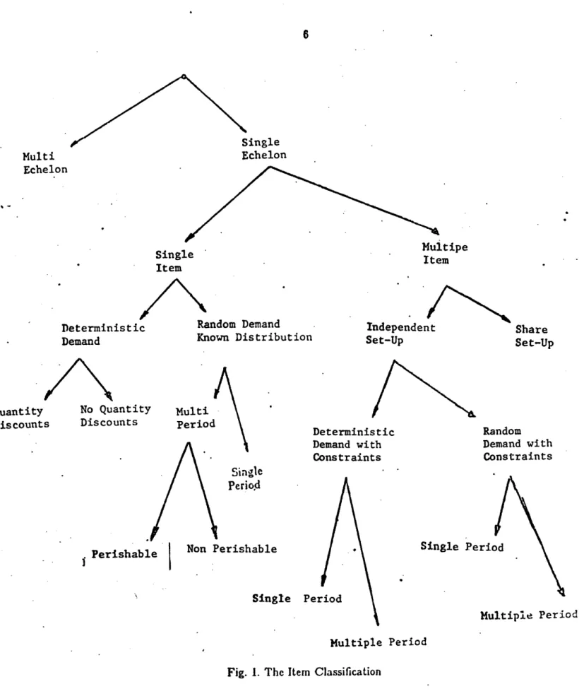
The proposed procedure starts with a simple gross classification that divides the population into a number of classes (sub-populations.) Estimates of the aggregate parameters of interest are computed using aggregate models and/or statistical sampling. In subsequent steps, the classes that present high internal variance are subdivided into more homogeneous subclasses. The subdivision of classes in different steps leads to the concept of a hierarchy of properties. In order to construct such a hierarchy, we have used the taxonomy represented in Fig. 1, based on Silver [16].
The cross reference of all the individual characteristics listed in [16] would generate an enormous number of classes. Instead, we propose in this paper to consider only the classes shown in fig.l. They represent the majority of algorithms in the literature and cover many of the cases encountered in practice. It should be kept in mind, though, that in some diagnostic analyses we may not have to go all the way down to each of the terminal points of the classification tree, whereas, in some others cases, even exhausting the classification power, the sample variance obtained may be so high that larger sample sizes will have to be used. Note that the strategy of analyzing the whole item set as if it were an homogeneous population fits in the proposed scheme, since such action is equivalent to stopping the classification at the first node of the tree.
4.- ESTIMATION OF THE AGGREGATE PARAMETERS
After dividing the population as described in section 3, we are left with a number of classes which contain iteins that share some qualitative properties. Nevertheless, items with very different total sales may coexist in the same set.
Two prollems arise at this point: first, it must be decided, for each sub-population, if an aggregate model will be used or statistical sampling will be performed. Second, if a decision to sample a given class
6 ;ingle Echelon Multi Echelon Single Item
Deterministic Random Demand
Demand Known Distribution
Multipe Item Independent Set-Up No Quantity Discounts Multi Period 1~ Deterministic Demand with Constraints Random Demand with Constraints Single Period
Non Perishable Single Perit
Perishable
1
Single Per
Multiple Period Multiple Period
Fig. I. The Item Classification
is made, we still have to cstimate a paranelter in a very skewed distribtli,. At the current state of the Quantity
Discounts
Share
Set-Up
research, aggregate models have been developed only for a few types of items. See for example [3] and [4].
If the number of items in a class is large, and no aggregate model is available, a statistical sampling procedure has to be used. In Proposition A.2 of the Appendix, we prove that under certain conditions, if zi is a particular attribute of item i (for example its cycle or safety stock), and X = N zi is the "class total" of attribute z, (N elements in the class), then, for a given sample size n, the variance of the estimate of X, X, is always smaller when we sample from a stratified population than when we consider the N items as a single class.
In the remainder of the paper we discuss and illustrate the diagnostic process of inventory systems. In particular we introduce a new technique to compute safety stocks as a function of forecast errors.
5. IMPLEMENTATION METHODOLOGY
An important problem arises with data collection. Although many corporations have computerized inventory control systems, they can rarely extract from their data bases the kind of information needed for a diagnosis study. Some properties like perishability, special promotions, planned withdrawals, etc., will in general have to be obtained directly from the manager of the system.
Figure 2. displays in broad terms the flow chart of the methodology we suggest in order to implement the statistical approach.
Two major steps can be identified: The estimation of cycle and safety stocks. Initially, we recognize, with the help of management, the set of items to which special attention should be devoted. Usual examples include items that will be removed from the product line or will be heavily promoted. In general, we should ask the information that can not be derived from the observation of the past behavior of the item. At this point, the analyst must decide at which level of the classification tree of figure I the study will be performed. In each box, either the whole population or a sample can be used. In order to. make this decision it is useful to realize that a sample size of at least thirty elements per class is required to obtain
we sample"
Yes
Draw sample "proportionals" to each class size.
Compute cycle stock.
Group in a single class all items in the sample
-Fig. 2. The Statistical Approach.
reasonable normal distribution approximations. With this data, cycle stocks can be estimated using the models available in the literature.
The next step is to estimate safety stocks in the absence of reliable information on the seasonality patterns of the products, we treat the whole sampile (or population) as a single class, and apply the
procedure of section 6. The algorithm outlined in subsection 6.3 groups, in classes, the items according to the behavior of their demands. If in each class the number of elements is smaller than thirty, a larger initial sample should be considered.
6.- A SYSTEMATIC PROCEDURE OF ESTINIATING FORECAST ERRORS
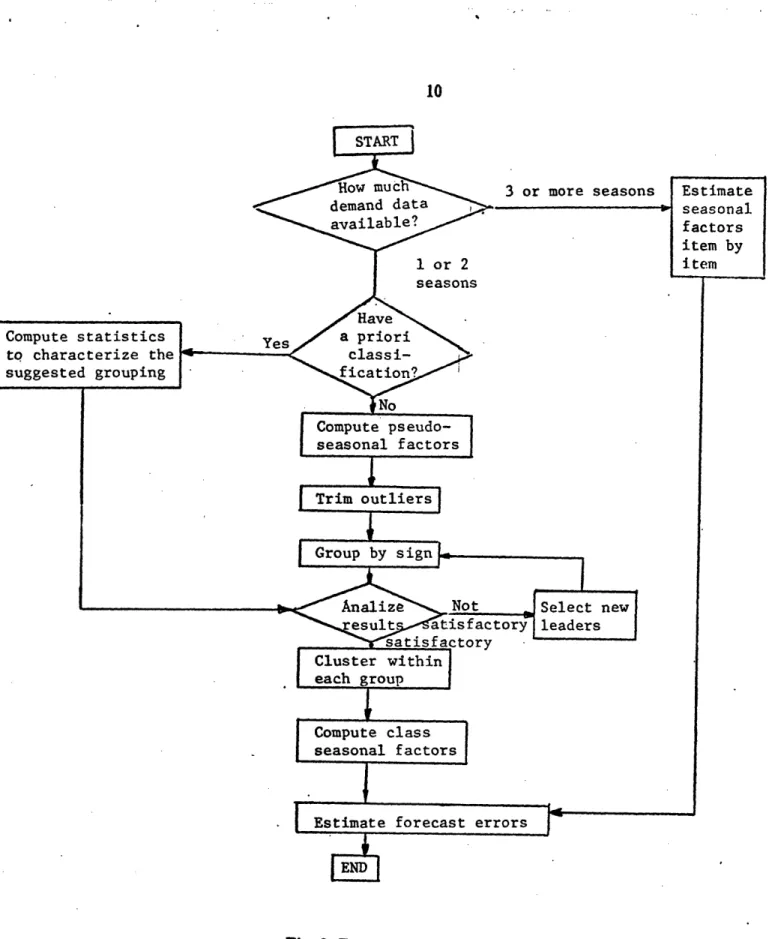
In order to estimate the safety stock that a company should carry to maintain a desired service level, it is necessary to know the magnitude of the forecast errors of its products, [5], [14]. In this section we introduce a systematic procedure to estimate both the seasonal factors and the forecast errors for a given set of items. The procedure, as described in the flowchart of fig.3, combines both objective statistical techniques and subjective managerial interaction. It applies to any set of items, either the whole population or a sample, depending on the branch we entered the box "Estimate the Forecast Errors" in figure 2.
The methodology is based on a simulation of the performance of a forecasting algorithm with observed demands; this simulation may be run using any of the forecasting techniques available, and in fact, it may be done with several of them to evaluate their performance in the particular system. In order to apply a forecasting technique to a given item, it is usually necessary to have estimates of its seasonal factors and trend. The estimation of the seasonal factors is a major task in itself, and takes most of the effort of the algorithm described in figure 3. The procedure is slightly different depending on the amount of data readily available:
- If three or more full seasons of demands are available, we use the most recent three to estimate the seasonality of each item separately. Section 6.1 details the procedure used.
- If only one or two seasons of demand data are available, we do not have enough degrees of freedom to estimate the seasonal factors itemn by item, 121. Only if we have additional a priori information of which items have the same seasonal behavior will we have sufficient data to compute estimates of their seasonalitics. This a priori knocledge is rarely available, and when it is, it should be carefully checked. The proposed procedure comiputes rough estimates of the seasonal factors for each item indepcnldently,
Compute statistics to characterize the -suggested grouping START Row much demand data available? 1 or 2 seasons Have Yes / a priori classi-ficatio I _No Compute pseudo-seasonal factors Trim
l~~~~~
outliers 3 or more seasons I Group by sign [~~~-Analize Not - Select new
esultx attisfactory leaders
satisfactory Cluster within each groupCo pt.l s
Compute class l
seasonal factors
I |LEstimate forecast errors
Fig. 3. Forecast Errors Estimation
the "pseudo seasonal factors" (psf's). Although such estimates incorporate all the noise present in the actual observations of the denmands, they reflect tile general shape of the seasolal variations, and are good
Estimate seasonal factors item by item _ __-., _
L.
_. 1 .4enough to be used to group items with similar demand profile.
The specific computation of the pseudo seasonal factors is explained in 6.2. The grouping of seemingly alike sets of pseudo seasonal factors is performed by means of a two steps clustering technique, and it is described in section 6.3.
Once the population is partitioned into sets of items with similar demand behavior, their common seasonal factors can be estimated. The particular computations are detailed in 6.4.
-If less than one full season of data is available, there is little that we can statistically do to compute the seasonal factors. We would have to rely on the behavior of related products and the information given by the managers of the system.
6.1 - ITEM BY ITEM SEASONAL FACTORS ESTIMATION
The seasonal factors used in this study are the multiplicative seasonal factors defined by Winters [22]. The multiplicative seasonal model is appropriate for time series in which the amplitude of the seasonal pattern is proportional to the average level of the series. This is usually assumed to be the case in demand data. The procedure to estimate the seasonal factors from at least three full seasons of data is based on the methodology proposed by Montgomery and Johnson 112] adapted to make use of more "resistant" techniques. A statistical summary of a data set is usually called resistant when it is not very much affected by wide variations introduced by single elements of the set, see Mosteller and Tukey [ll]. For example, a resistant version of the mean, as a summary location parameter, is the median.
We illustrate de procedure with the following model:
yl = (b( + bt)sA + l
where y,, b,, bl, s and (, are respectively the sales, the base value, the linear trend, the multiplicative seasonal factor, and the randomn error component.
12
If the length of the season is L, the seasonal factors are defined in such a way that:
L
ft- l We estimate the sft's as follows:
- First estimate the trend b as the slope of the line that connects the median sales of the first and the last season of available data. For example, if we have m years (seasons) worth of data, and Pl, P2-. .m
denote the median.sales for each season, the estimate of b1would be:
1= m-y
(m- 1)L
As stated earlier, the reason for using the median instead of the mean is that we can expect the presence of very large or very low demands in the time series that are in fact not due to seasonal variations, but to unpredictable events. Therefore, they should not be incorporated to the estimation of the seasonal factors; in other words, the model should not try to explain accidentarvariations that most likely do not follow the main seasonal pattern.
- Estimate the base value as the average of the differences between the slope and the summary points:
I _ L(2j - 1)
m
(.
2)
- Compute the estimates of the seasonal factors period by period (mL of them):
;I, = o + t (t = 1, 2,..., mL)
- Average all estimates of the same seasonal factor:
Jft
E St+(i-I)L
= (t 1, 2, . .,L)j=1
- Finally, normalize the seasonal factors so that they add to L:
S = L (t=-1,2,..., L)
6.2 - COMPUTATION OF THE PSEUDO-SEASONAL FACTORS
The pseudo seasonal factors are used as a first approximation to the real seasonal factors that can not be effectively computed because there is only one season of data for each item. They are used to group items that have similar seasonal behavior. The pseudo seasonal factors should be computed only for the items that do not present a long span of zero demand. The analyst should in each particular situation decide when an item ought to be considered a single season sales item, and therefore deserves separate attention.
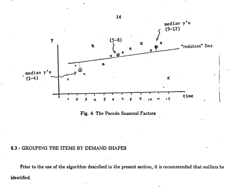
As shown in Figure 4, we compute the pseudo seasonal factors as the standardized residuals of a resistant linear model. A resistant line was chosen over a traditional least squares regression line because of the very noisy nature of the data, that would make the model try to explain exceedingly high or low sales, and therefore would deteriorate the goodness of the whole set of psf's. For a discussion of the properties of resistant regression, see Vellman and Hoagin [18]. The technique and the computation of the psf's consist of the following steps:
- Divide the time horizon into three equal length time periods.
- Find the median of the sales in each division and define the "summary points" (median time period, median sales) for each third. Note that for a twelve month data set, the medians of the time (the explanatory variable), are for each third 2.5, 6.5, and 10.5. Let us denote the three summary points by
(xi, yt), (m, y,,) and (, a) respectively from early time periods to later time periods. - Estimate the slope of the resistant line b from the end summary points:
__ -- X - Calculate the intercept:
a [(YI - 6Xi) + (,m - bX,.) + (h bXh)l
- Compute the psf's:
median Y' s (9-12) y (5-8) V IV -median y' s (1-4) esistant" line ime l I L J 4 5 & 1 g' " '
Fig. 4. The Pseudo Seasonal Factors
6.3 - GROUPING THE ITEMS BY DEMAND SHAPES
Prior to the use of the algorithm described in the present section, it is recommended that outliers be identified.
Non seasonal items:
Items with many changes of sign in the psf's should be considered non seasonal due to their erratic behavior. The analyst should decide in each case when to consider an item to be non seasonal; note for instance that up to four changes of sign include items with two high selling seasons.
Outliers reduction:
To detect sorie of the often unpredictable, non stationary peaks or drops in sales, we compute, for each month, the "outside" and "far out" psf's of the whole population, and bring them to the monthly
inner fence".The nomenclature and concepts conform to Tukey [17].
When some a priori knowledge about possible grouping of the items by seasonalities is available, we still compute the pseudo seasonal factors as indicated in section 7.2, but the trimming is done class by class instead of to the overall sample at once.
The following definition is used in what follows:
Definition
The "sign distance" between two time series t, t = 1, 2,..., T and /l, t = 1, 2,..., T, is defined as D(x, y) = dsign(, t) t=l where 0, { if uv > 0 dsign(u, v) = < t1, if uV < 0
Note that the distance between two time series of T periods is bounded by zero and T. The distance is zero when the sign of'the elements of the two series are the same period by period (or at least one of them is zero), and it is T when all elements are nonzero and there is no agreement between their signs in any period. The distance between two items will be small whenever their demand profiles go "up and down" in the same phase, regardless of their amplitude.
In order to group the items that have the same demand shape, the following variation of the leaders algorithm described in Hartigan 17] is used:
- Select several leaders or "fundamental demand shapes" with the help of the manager of the company or according to past experience. The leaders are represented as series of ones and minus ones. For example, a leader consisting of ones from period one to six and minus ones thereafter, will match with items in the population that have high sales from January to June and low sales from July to December.
- For each item in the population, compute the "sign distance" between its sequence of pseudo seasonal factors and each leader.
- Assigi the item to the closest leader.
Note that this is equivalent to putting in the same class all the items that have high sales and low sales in the samne periods disregarding their relative variation.
band around zero. Since the distance of zero to any number is zero according to the definition of the sign distance, this procedure tends to reduce the number of errors induced by the noise inherent to the data. Under the assumption that the leaders selected by the managers truly represent all the fundamental seasonal patterns in the population, it can be shown that the classification rule stated above selects the maximum likelihood estimator of the pattern to which a particular item belongs. This'is formally stated and proved in what follows.
Given a sequence {t} let
3+1, if t >0 ign(xt)- 0, if = -1, if zt < 0 Assumptions:
1) The time series formed by the signs of the seasonal factors of any item in the population is equal to one of the defined leaders. Let us call I the set of L leaders, each one a time series of T elements with components I or -1:
~'v={{ , 4,2, ,A,} .. ; 1=1,2, ... , L}
2) Our observation of the signs of the pseudo seasonal factors {psfi,psb,...,psfT}, for the item
considered, is one of the leaders I E P affected by an error component of the form:
sign(psft) = ,tet and where
f+1, with probability p+
= O. with probability Po
-1, with probability p_
p+ > p_, and t t = 1,2,..., T are independent identically distributed random variables. The error component t needs not be the same for all items. For simplicity of notation we will denote sign(psfi) by PSf
Proposition 6.1:
The maximum likelihood estimator i of the leader that generated the observation {psf, psf2, ... , psfr}
is the i E I such that the sign distance D(psf, i) in the minimum for all elements of If.
Proof:
The likelihood function f(p7fjl), the probability that the leader generated the observation psf, is:
fJ
I)=
II
P+
II
PoII
-P ft4tt pJJ,0 pi=--zBt
But, since D(psf, 1) is "counting" the number of times the leader I and the signs of the observed pseudo seasonal factors have the opposite sign, we can rewrite,
f(ijil) =cp1( perioda with right *ign)p of zeroea)p( wrong ign)=
= pp nopD(psfuI) = pTnoD(psfl)noD(psfl) =
= T (o )no( P-)D(paf t)
+ maximum I will be:likelihood estimator P+the of
Therefore, the maximum likelihood estimator of I will be:
max f(ps71f) - maxp+;( P -)D(psl) = IEE* P+ P+ = p(+)-O maOX(P-)D(pfI) = p+ p+ = p (
u, ),,( P-),ni.n uxzJl,) =
_= 7'.! )""( I)(p )P- fi)-t1i) P+ p+ ______1__1__111__I___ __18
where
D(psf, i) = min D(psf, 1) I
Two displays are presented in order to determine if the chosen leaders are fully representative of the main profiles present in the population.
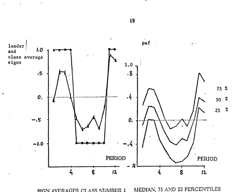
Figs. 5. and 6. present a typical output corresponding to one leader. Fig. 5. shows the leader in the squared points and the average sign of all items in the class month by month. The intent of the plot is to show how close the items of the class are to their leader considering only the sign of their pseudo seasonal factors. Average values near to those specified for the leader imply that most of the items have the expected sign, and average values in the opposite side of the zero line, imply that more items have the wrong sign in the period in question.
Figure 6. plots the median of the psfs in the class for each month, together with the 25 and 75 percentiles.
With those plots the analyst is able to decide if the leader of the class has in fact a substantial chunk of the item population following it. A few trials are enough in most practical cases to determine a reasonably good set of leaders.
Up to this point we have divided the set of items under analysis into classes of items that present the same shape of seasonal pattern but that may differ regarding the amplitude of the variation. The next step is to unify such amplitudes, that is, group the items (whitin each class formed by the leaders algorithm), that have close relative variation with respect to the average demand. This will allow us to hypothesize that all items that fall in the same class have the same multiplicative seasonal factors.
This second grouping is done via the hybrid clustering algorithm described by Wong 1231. This algorithm does not require either a priori determination of the number of clusters nor a set of arbitrary
"centers". It tries to identify natural breaking points in the spectrum of different seasonal amplitudes. Ini the situations where there is a dense set of internlcdiate values of amplitudes, the algorithm may be unable to find such natural gaps to divide the population. In this case, if the difference between th; "most"
leader and 1.0 class average signs .5 0. -1.0 psf 1.0
.8
.4
0. PERIOD4
Z1 75 % 50 % 25 % IOD 4 8 12.. SIGN AVERAGES CLASS NUMBER 1I MEDIAN, 75 AND 25 PERCENTILES
Fig. 5. Leaders Evaluation Fig. 6. Leaders Evaluation
and the "least" seasonal item is large enough so that we can not assume that their difference is due to randomness, the population in the class must be divided into strata by the analyst.
6.4 - COMPI'UTATION OF THE CLASS SEASONAL FACTORS
The result of the hybrid clustering algorithm is a set of groups of items that present similar seasonal behavior. At this point, it is not unreasonal;le to assume for practical purposes that all items in the same
1
-. 4
--20
cluster have the same seasonal factors, and that the differences they present are due to unpredictable variations. We are therefore able to compute estimates of the seasonal factors for the items in the cluster. A procedure similar to the one described in 6.1 for several observations of the same item can be used. It has to be adjusted to the fact that now, different observations come from different items and therefore, their trends and base values need not to be the same.
The computations reduce to averaging the pseudo seasonal factors of all the items in the class. These averages are directly supplied by the cluster analysis algorithm. Only a scaling in order to get them to add to the length of the season, usually twelve, is needed.
Forecast-Errors Estimation
With the estimates of the seasonal factors on hand, we can apply the desired forecasting algorithm. The period by period standard errors of such simulation are the estimates of the forecast errors of the item. We illustrate this procedure with actual data in the next section.
7. AN APPLICATION
7.1. - DESCRIPTION OF THE DATA SET
In this section we illustrate the procedures detailed in the previous sections by applying them to a set of 7464 items drawn from a real situation. In this application the whole population is used for the determination of seasonal patterns and forecast errors, but we recur to stratified sampling to estimate cycle and safety stocks.
The data was obtained from a wholesaler firm interested in evaluating the performance of its own inventory control system. In particular, the management of the company wanted to know whether it was possible to improve the service level given to customers without increasing their current annual inventory holding cost of 60 million dollars. The aim of the analysis was to estimate cycle stocks and tile forecast
errors attainable by an exponential smoothing technique, and to compute the maximum service level (as
expected proportion of serviceable (lenland) that could be delivered with the aforementioned suml of GO
21
million dollars.
The structure of the product line and the information provided for the analysis can be summarized as follows:
a) NMulti-Period Items. A total of 6479 items fall into this category. They are non-perishable items. For each of these items, twelve observations of monthly demand and their corresponding holding and set up cost are available.
Out of the 6479 items contained in this category, 1514 are "independent" items. An item is called independent whenever there are no economies of scale in ordering it together with any other item in the whole population. The remaining 4965 items belong to 85 families. A family is composed of a number of items sharing the same ordering cost. A given family contains anywhere from 200 to 45 items.
b) Single-Period Items. The remaining items, a total of 985, have a single non-zero demand period. The company, therefore, either has to keep the non-sold items in stock for a full year, or has to sell them under-priced. For each of these items, estimates of their expected annual sales and their variability, as well as under and over stock costs are known. Single-period items represented a very small percentage of the total demand, only 1.4%.
7.2. - ESTIMATION OF THE FORECAST ERRORS
The algorithm described in section 6 was applied to the whole population of 6479 multi-period items. The first step, according to Fig 3, consisted in determining the pseudo seasonal factors. Next, a program to check for the presence of non-seasonal items (more than four changes of sign) was run. 1485 items were found with erratic behavior and removed from the analysis, with their multiplicative seasonal factors set to 1 for all time periods. The same program computes the.hinges of the pseudo seasonal factors period by period and reduces the outliers to the outer fences (nomenclature follows Tukey 1171.) A sumninary of the redluctions made is shown in the table of figure 7, where the values of tile fences and the number of
items trimmed on each side are displayed.
The next step was to identify the fundamental shapes or leaders for the classification. Given the nature of the company and with the aid of its management it was decided before the start of the analysis that eight fundamental shapes of demand representing all items was a reasonable first guess.
The eight "leaders" chosen were: 1: high winter demand (November to April)
2: high spring and fall demand (March to May and September to November) 3: high summer and winter demand (December to February and June to August) 4: high summer demand (May to October)
5: high peak summer demand (June to August) 6: high spring demand (March to May)
7: high peak winter demand (December to February) 8: high fall demand (September to November)
After the trimming, the classification algorithm itself was run. It partitioned the population into eight classes, one for each leader.' The results of the classification are shown in figure 8. The two entries of the table are the class number and the sign distance to its leader. For each class, the number of items that are at a given distance is displayed.
Of the plots made to judge the goodness of the leaders, only those corresponding to leader number one are discussed here. They were shown in figures 5 and 6. In figure 5, the leader is plotted withl square points, and the average sign of the class with triangles. In January (month one) we observe that the fit is quite poor: The leader has a plus one, but more items have low demand (negative sign) than high demand. On the other hand, in November, for example, a large number of the items have high demand, and therefore, follow its leader.
A better appreciation of the homogeneity of the items in the class may be obtained froin Fig.6. It represents the 25 percentile, median and 75 percentile of the true seasonal factor. (This median should not
TRIMMIED 152 e3 /41 62 /22 l3' 150
96
200 1802.4T
I
L
7
K
I
I
LA_
-2 -2 38 24 -.9
5-1.85
.79-2.01
g o 2.36I
-2.09q
0 0 2.13 -2.2q9 2.7rr
I
- 2,48 J9 -2.oZ 1,8Z -)93 0 0 0 # OF ITEMSI TRIMMEDFig. 7. Pseudo Seasonal Factors Statistics Period by Period
DSIGN DISTANCE .. CLS;-S- : .-
o:
.. I - : 32 0 . s ~ f .~~* a 3 1 4 .... 5: TOTAI. Ii 14: 96 * 3: 10: * _ 4: 21: 5: 19: * . 6: 5: 7 : 25: * B: 2: 67 51 91 105 80 I 200I 131: : . 81: 200: 262: i00: 23: 31: 139: 1591 42: 1171 85: 178 299: 332: 337: 355: 483: 36: 55: 75: 143: 246:Fig. 8. Classification Summary Statistics
be coirfused x itii the "sign" average represented in figure 5.) Exaniniing Fig.G, we see thai in almost all
123 116 0. Lo
-,,44
q 3t 42. 0 3: 3: 8: 15: 23: 376: 2681 553: 790: 837: 86'3: 796: I_____ II
1
)-193 484s _ . _ _ I Imonths, more than 75 percent of the items have the right sign in the pseudo seasonal factor. Particularly good are June, September and November.
After analyzing the results of the assignment algorithrm for all eight leaders, it was decided that they represented well enough the item population, and that they could be kept as the true "representatives" of all possible demand shapes. The poor fit that is observed in period one, not only for leader number one shown here but for all the leaders that call for high demand in the first period, was explained by the managers of the company as due to exceptional circumstances (a strike) which forced the sales to be much lower than usual for all items.
With the items grouped by demand shapes, the next step was to subdivide the classes with regard to the absolute value of their seasonalities. This was done according to the Euclidean distance between time series of pseudo seasonal factors. The clustering algorithm of Wong 123] was used for that purpose. The algorithm tries to identify natural groups among all items belonging to the same class. In our case the algorithm was not able to differentiate natural partition points in any of the eight classes. In those cases, the conclusion is that there is a continuum between the most seasonal of the items and those having the most uniform demands. Following the recommended procedures for such instances, we divided each class into four subclasses containing items with close relative variation. The thirty two classes obtained captured satisfactorily the characteristics of the items under study. This subdivision was done using the k-means method 17] incorporated in Wong's algorithm [23].
After this last classification, we hypothesized that ali the items in the same subclass have the same multiplicative seasonal factors. With such hypothesis, the estimation of the seasonal factors was done according the procedure described in 6.4.
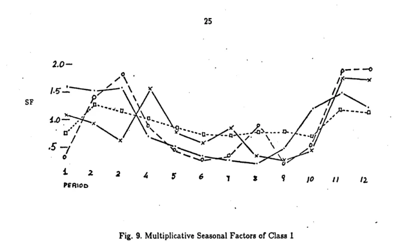
The results, for class one, are displayed in Fig.9. As expected, the four sets of seasonal factors have the same general shape as the leader . The "square" series belong to the least seasonal iteins while the "black dots" correspond to the most varying one. An interesting point is risen by the "circle" seasonal factors set; note that the January seasonal factor is the lowest in the whole group, and moreover, it is in
2.0-. P- - -O .0-.5 -i 2 2 4 6 8 9 O 11 12 P6sRoD
Fig. 9. Multiplicative Seasonal Factors of Class I
contradiction with the leader. A close examination of the items contained in this subclass, showed that a large number of them had zero demand in January, but the rest of the year clearly conforms with the high winter sales item.
Once a set of seasonal factors has been assigned to each item, the simulation detailed in section 6.5 was run. The forecasting technique used was the exponential smoothing of Winters 122] with a = .3 for
the first three periods and a = .2 thereafter.
7.3. - ESTIMATION OF TIE LEVELS OF CYCLE AND SAFETY STOCK
The taxonomy of figure 1 was applied to our data set. As commented earlier, only three clearly different classes were present. The properties of the items in each class were:
a) Single item . Random Demand Known Distribution . Multi-period . Non-perishable. b) Multiple items. Random Demand Known Distribution . Multi--period . Non-perishable. c) Single item. Random Demand Known Distribution . Single period.
__~~~~~~~~~---26
The items that fall in each class were analyzed as follows:
a) This class consisted of 1514 items. It was reasonable to assume that a moderately sophisticated inventory control system would model the behavior of these items using the Dynamic Programming technique of Wagner and Within [20].
An exhaustive simulation would require the solution of 1514 dynamic programs. This is not an extraordinary number of problems to be solved, but for illustrative purposes, we decided to sample this class. Prior to the sampling, and according to the procedure detailed in section 5, the items were sorted by demand and divided into four strata. A proportional sample of 150 items was chosen, and the simulation run. The random fluctuation of the demand was absorbed by a safety stock.
b) 85 families of items were present in this class. It was assumed that the random component of the demand of the individual items was absorbed by a safety stock. The sets of items in each family, share ordering costs and have deterministic varying demands. These are the conditions required to apply the aggregate algorithm described in section 2.2 of [3].
The company under study computes inventory holding costs as a fixed proportion of the value of the item. In our application, the unit inventory holding costs were constant over time. As stated in Proposition 2.8 of [3], this is a sufficient condition to guarantee the optimality of the aggregate model.
Given that the number of families was only 85, it was decided to use them all in the analisys. This class, therefore, did not add any variance to the total inventory estimates.
c) The same sampling procedure described in (a) was used to select 200 items out of the 985 in the single season class. They were modeled using the classical news-boy algorithm [14].
7.4. - RESULTS OF TIlE SIMULATION
The results of the simulation are summarized as follows (K is the factor that nmultiplies the standard deviation of the forecast error in order to compute the safety stock level, and for illustrative purposes it
is assumed constant for all items):
Independent Multiple Period Items: E[Total Cycle Stock] = 20.38 Million Dollars; ac s = 2.26 1012
Dollars; E[Total Safety Stock] = 2.66 K Million Dollars; oss = .23 1012K2 Dollars;
Multiple Item Multiple Period Families: Total Cycle Stock = 25.45 Million Dollars; Total Safety Stock = 1.98 K Million Dollars;
Single Period Items: E[Total Stock] = .29 Million Dollars; oTs = 56 10nDollars;
TOTALS: Total Cycle Stock = 46.12 Million Dollars; orcs = 1.50 108 Dollars; Total Safety Stock = 4.64 K Million Dollars; arss = .48 K 106 Dollars.
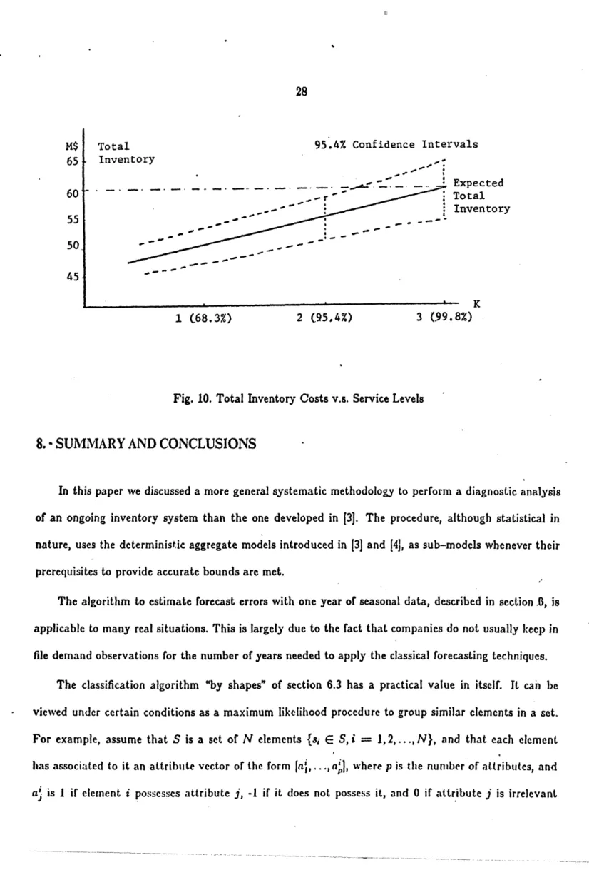
Therefore, assuming that our estimates of the cycle and safety stocks are estimates of independent random variables, the 95;4% confidence intervals of the total inventory (TI) as a function of K are (Note that the contribution to the total variance of the single-period items is negligible):
Pr(46.12 + 4.64K - 2(2.26 + .23K2) < TI < 46.12 + 4.64K + 2(2.26 + .23K2) = .9546
A graphic representation of this interval is given in figure 10.
Observing the graph in figure 10, we can phrase the conclusion of our analysis as follows:
If the company sets its service level, constant throughout the population, at 99.8%, and uses the Wagner-Within and News-Boy algorithms to compute lot sizes for the appropriate items, the expected total inventory cost will be the current figure of 60 Million Dollars. On the other hand, if the service level is set at 95.4%, there is a .954 probability that the total inventory cost will be between 58.9 and 51.8 Million Dollars.
Figure 11 allows the management of the company to set service levels according to the desired inven-tory investments. This graph is an example of the so called trade-off curves already popular in inveninven-tory control theory 161,I11, with the inmportant addition of confidence intervals.
28 MS 65 60' 55 50 45
Total 95.4% Confidence Intervals
Inventory Expected _c _,~~~ r Total _,-' . Inventory L _ _ _ _ _c _--^~~~~~~~~~~~~~~~~~~~~~~~ c ~ ~ ~ .- 1 (68.3%) 2 (.95,4%) 3 (99.8%)
Fig. 10. Total Inventory Costs v.s. Service Levels
8. SUMMARY AND CONCLUSIONS
In this paper we discussed a more general systematic methodology to perform a diagnostic analysis of an ongoing inventory system than the one developed in 3]. The procedure, although statistical in nature, uses the deterministic aggregate models introduced in 3] and [4J, as sub-models whenever their prerequisites to provide accurate bounds are met.
The algorithm to estimate forecast errors with one year of seasonal data, described in section.6, is applicable to many real situations. This is largely due to the fact that companies do not usually keep in file demand observations for the number of years needed to apply the classical forecasting techniques.
The classification algorithm "by shapes" of section 6.3 has a practical value in itself. It can be viewed under certain conditions as a maximum likelihood procedure to group similar elements in a set. For example, assume that S is a set of N elements {si E S, i = 1,2,..., N}, and that each element has associated to it an attribute vector of the form I[a,. .., ap, where p is the number of alttribules, and a. is I if element i possesses attribute j, -1 if it does not possess it, and 0 if attribute j is irrelevant
to item i. Assume further that we are able to define a set of L leader-vectors with p attributes which observations are subject to errors of the same nature as those described at the end of section 6. Under these circumstances, it readily follows that Proposition 6.1 holds, and therefore the algorithm of section 6.3 performs a maximum likelihood grouping of the elements of S around the L leaders.
ACKNOWLEDGMENTS
The authors are grateful to Professor M. Anthony Wong for his insightful comments on statistical clustering, and to Professor Stephen C. Graves for reviewing an earlier version of the manuscript.
--"---30
APPENDIX
Proposition A.1.:
If a E [0, 1), b E (0, 1] and s E (0, 1), then
-- (bS+ _ f+1)2 (Y+ -_a+1)2 (b'+l _- as+ )
+ -a - b-a0 >
b -- I VI - y° ala b'
-for all a < y < b. Proof:
Since y E (a, b), yI E (a', b8). Therefore, at least one of the following cases hold:
1) b - V' < Vy - a
2) b - yI y - a'
Assume 1) holds. Then
A>
(b+ _ +1)2 (y+l _- a+l)2 (b8+l - as+])2>
-
> 0
- '/-a
+
y -a y - a"by the triangular inequality and b' - a' > y - a'.
In case 2),
>
(b+ - yA+1)2 (ya+l _ oa'+l)2 (b'+l _ a_+)
> 0
- b- -
+
b - VI bs - eby the triangular inequality and b - y > b - a' i.
Definitions and Assumptions:
The following assumptions will be used throughout this appendix: - The analysis is performed with a family of N items.
- xi E i = 1, 2,..., N denote the value of a given attribute of ilemin i. Examples of such attribute are cycle inventory, dollar usage, etc.
- The possible values of xi are bounded by 0 and M (0 < zi < M).
- The parameter of interest is X = zi, x- the class total of the attribute.
- Although we have a finite number of items in the population, we will assume that N is sufficiently large to justify the approximation of treating the attribute X as a continuous random variable.
- The cumulative distribution of the item attribute x, for the population of the N items is given by:
oes
P(z ~z)= a E(O,1).
That is, the underlying distribution is of the form:
f(Z) = M z ,E M
This distribution has been found, by Hausman et al. [81, to fit fairly accurately the classical "ABC" curves present in inventory problems.
Let Xh, Xh, Xu and Xp be respectively the total of the attribute in strata h, its estimate, the estimate of the population total computed by uniform sampling, and the estimate of the population total by proportionally allocated stratified random sampling. In addition, let fl be a partition of the interval of variation of attribute x
fI= {, z, ,..., L,M} ; <z i if i<j
that is, a partition of [0, MA] in L subintervals [0, z), zi, z2),..., [ZL-, AMI. For each partition , let (Nj) -_
l
with I Nj = N denote the number of items that fall into each subclass. A sample of size n is said to be "proportionally allocated" among strata Qf if the number of items sampled in a particular class 1, tt, is proportional to A/t, that is:nl n2 nL n
NJ N" NL N
Proposition A.2.:
For a given sample size n, the variance of the estimate of the class total, , for any partition and proportional allocation of the sample, is always smaller than the one obtained by uniform sampling on the interval [0, Mi.
Proof:
When sampling with replacement, the variance of
fru
(uniform sampling) is given by the expression, (Yamane [23]):V(Xu)= N2NN' n
where v2 is the variance of the attribute z. Since
v2 = El[2] -(E[Xl) 2, M f M 2 Ebzl2 2 l= 2(z)d f = J
L
+Mdzs +2 12x+2t = - +M2 and 8+1 E ]_ .tM x )dx 1 s- d a M It follows that N(N - n) j (2 V( ) n 8---M o + 2 ( - + 1)2On the other hand, using proportional allocation, the value of the variance Xp is given by:
L n
where Nh and v2are respectively the number of items and the variance on the attribute z in strata h. The value of vh2can be readily computed considering that the distribution of z in the interval [z,-I.,zh), strata h, is of the form:
IKh I
or, fh(Z)= z z_ ~h - ZhA-I Since - - =_ 8 Z dz ~-
--4--
-I + I .-4- Z l andEh[X2]
~EhI1=
2 ' =L z2fh(x)dz = =8 'd h-zI-
ZA,_
_,-s
+ 2 - zl,,82
(k + 1)2
2 + + 2 2h -z° +2 _z,+2h-1 Zh - h-I and therefore, = N-P N 8 -a+2 zh-e_The number of items in strata h, interval [zh-, z,), because of the continuity approximation, can be computed as:
Nh = N f(z)dz = M( - k-I)
which leads to:
V(~ ) N-n
n
L N a J +2 +2 h iM~l82 h h-1 n Ms 8,i +2 -I 82 (Ze+ I-Zh )2 (' + 1)2 Zh-Zhs-I 8a 2 1 a + 2 (s + 1)2 M+ 2Therefore, V((p) < V(ku) if and only if
1 L (Z.+ _ z t )2
FZ = k
E
( - q-';_-> 1.____ ____1_111__1________·
62 z8L+I -Z#,+J
In order to prove this inequality, let us define yh = D (note that h > k if and only if k > h.) Then, L Fn = MS+2 -h=1 L h=- 1h51l (yh+1 - --18+1)2 M28+2 Yh - Yh-l* Ms (Yh +l -- M_18+1)2 YhS - h-1 8
The proof of Fn > 1 for any partition is carried out by the following inductive argument:
1) Assume Ql = {O, yM, M), where y (0, 1), that is, nl is a non trivial two strata partition of
[O, M.
= (+1)2 (1 _-- +1)2 _ 1 = y+2 + 1 + y2a+2 _ 2dy+1
FOI-1 = y + I -- y1 y'
yd~~&'
-- =
*y+2 _ 2+2 + I + y2s+2_ 2y+I _ 1 + U
I--F
y2- 2y + I _ (i- 1)
> 0
-- to y,1-I
2) Assume that for a given partition QL of L intervals, the corresponding Fni, > I and that a new point yM is introduced between zk and zk+l creating the partition flL,y. Note that 0 < yJ < y < k+l < 1.
Thus, the difference between the new expression Fn,,. and Fn, is given by:
(k+i+1 -- y8+1)2 (y8+l - ko+)2
Y+1a - If -+ - Y/a
(yk+l8+l - ys+1)2
Yk+ Yk+l -V- Y
and, by proposition A.1. proved before:
FnL, -FnL Ž> 0
and consequently
FnL,y > I .
It is Nworth noting at this point that Xr,, is an unbiased estimator of the class total X:
If h is the estimate of the population total in strata h:
L L L
E|Xkp,=E
kh]=
E[Xh]
=
Xh-X
h=l h=l
h=The fact that E[Xh], the expected value of the estimate of the total in strata h is in fact Xh is a -consequence of the properties of uniform sampling within a strata. We have proven in this appendix that in order to estimate the aggregate attribute X, we obtain smaller variances using a stratified technique than sampling the whole population uniformly.
36
REFERENCES
11] Aitchison J. and Brown J. "TheLognormal Distribution" Monographs Cambridge University Press 5, (1957)
[2] Aggarwal S.C. "A Review of Current Inventory Theory and Its Applications" International Journal of Production Research 12,443-482 (1974)
[3] Bitran G.R., Hax A.C. and Valor-Sabatier J. "Diagnostic Analysis of Inventory Systems: An Optimization Approach" Naval Logistics Research Quarterly Forthcoming
[4] Bitran G.R., Magnanti T.L and Yanasse H.H. "Analysis of the Uncapacitated Dynamic Lot Size Problem" Sloan School of Management (1981)
[5] Brown R.G. Materials Management Systems John Wiley & Sons, New York, N.Y. (1977) [6] Brown RG. "Estimating Aggregate Inventory Standards" Naval Research Logistics Quarterly
55-71, (May 1963)
[7] Hartigan J.A. "Clustering Algorithms" John Wiley and Sons New York (1975)
[8] Hausman W.H., Schwarz L.B. and Graves S.C. "Optimal Storage Assignment 'in Automatic Warehousing Systems" Management Science 22, 629-638 (February 1976)
[9] Hax A.C. "A Comment on the Distribution System Simulator" Management Science 21, 232-236 (October 1974)
[10] Hax A.C., Majluf N.S. and Pendrock M. "Diagnostic Analysis of a Production and Distribution System" Management Science 26, 171-189 (September 1980)
[11] Mosteller F. and Tukey J.W. Data Analysis and Regression Addison-Wesley, Philippines 1977
[12] Montgomery D.C. and Johnson L.A. Forecasting and Time Series Analysis McGraw-Hill, New York 1976
9, 447-483, (1978)
[14] Peterson R. and Silver E.A. Decision Systems for Inventory Management and Production Planning John Wiley & Sons, New York, N.Y. (1979)
[15] Raj D. Sampling Theory McGraw Hill. (1968)
[16] Silver E.A. "Inventory Management. A Review and Critique." To appear in Operations Research (1981)
[17] Tukey J.W. Exploratory Data Analysis Addison-Wesley, Philippines (1977)
[18] Vellman P.F. and Hoaglin D.C. Applications, Basics, and Computing of Exploratory Data Analysis Duxbury Press, Boston (1981)
[19] Wagner H.M. "Research Portfolio for Inventory Management and Production Planning Systems" Operations Research 28, 445-475 (May-June 1980)
[201 Wagner H.M. and Whitin T.M. "Dynamic Version of the Economic Lot Size Model" Management Science 5, 89-96 (October 1958)
[21] Wharton F. "On Estimating Aggregate Inventory Characteristics" Operational Research Quarterly 26, 543-551 (1975)
[22] Winters P.R. "Forecasting Salesby Exponentially Weighted Moving Averages" Management Science 6, 324-342 (1960)
[23] Wong M.A. A Hybrid Clustering Algorithm for Identifying Iigh Density Clusters Sloan School of Management Working Paper No. 2001-80, January 1980
[24] Yamane T. ElementarySampling Theory Prentice-Hall, Inc., Englewood Cliffs, N.J.(1967)