HAL Id: hal-00720424
https://hal.archives-ouvertes.fr/hal-00720424
Submitted on 24 Jul 2012
HAL is a multi-disciplinary open access
archive for the deposit and dissemination of
sci-entific research documents, whether they are
pub-lished or not. The documents may come from
teaching and research institutions in France or
abroad, or from public or private research centers.
L’archive ouverte pluridisciplinaire HAL, est
destinée au dépôt et à la diffusion de documents
scientifiques de niveau recherche, publiés ou non,
émanant des établissements d’enseignement et de
recherche français ou étrangers, des laboratoires
publics ou privés.
A Fuzzy-Cautious OWA Approach with Evidential
Reasoning
Deqiang Han, Jean Dezert, Jean-Marc Tacnet, Zhun-Ga Liu
To cite this version:
Deqiang Han, Jean Dezert, Jean-Marc Tacnet, Zhun-Ga Liu. A Fuzzy-Cautious OWA Approach with
Evidential Reasoning. Fusion 2012 - 15th International Conference on Information Fusion, Jul 2012,
Singapour, Singapore. pp.278-285. �hal-00720424�
A Fuzzy-Cautious OWA Approach
with Evidential Reasoning
Deqiang Han
Inst. of Integrated AutomationXi’an Jiaotong University Xi’an, China 710049
Jean Dezert
ONERAThe French Aerospace Lab F-91761 Palaiseau, France [email protected]
Jean-Marc Tacnet
Irstea, UR ETGR, 2 Rue de la papeterie-B.P. 76 F-38402 St-Martin-d’H`eres, France [email protected]Chongzhao Han
Inst. of Integrated AutomationXi’an Jiaotong University Xi’an, China 710049 [email protected]
Abstract—Multi-criteria decision making (MCDM) is to make
decisions in the presence of multiple criteria. To make a decision in the framework of MCDM under uncertainty, a novel fuzzy -Cautious OWA with evidential reasoning (FCOWA-ER) approach is proposed in this paper. Payoff matrix and belief functions of states of nature are used to generate the expected payoffs, based on which, two Fuzzy Membership Functions (FMFs) representing optimistic and pessimistic attitude, respectively can be obtained. Two basic belief assignments (bba’s) are then generated from the two FMFs. By evidence combination, a combined bba is obtained, which can be used to make the decision. There is no problem of weights selection in FCOWA-ER as in traditional OWA. When compared with other evidential reasoning-based OWA approaches such as COWA-ER, FCOWA-ER has lower computational cost and clearer physical meaning. Some experi-ments and related analyses are provided to justify our proposed FCOWA-ER.
Index Terms—Evidence theory, OWA, belief function,
uncer-tainty, decision making, information fusion.
I. INTRODUCTION
In real-life situations, decision making always encounters difficult multi-criteria problems [1]. In classical Multi-Criteria Decision Making (MCDM) framework, the ordered weighted averaging (OWA) approach proposed by Yager [2] has been increasingly used in wide range of successful applications for the aggregation of decision making problems such as image processing, fuzzy control, market prediction and expert sys-tems, etc [3]. OWA is a generalized mean operator providing flexibility in the aggregation. Thus the aggregation can be bounded between minimum and maximum operators. This flexibility of the OWA operator is implemented by using the concept of orness (optimism) [4], which is a surrogate for decision maker’s attitude. One important issue in the OWA aggregation is the determination of the associated weights. Many approaches [5]–[10] have been proposed to determine the weights in OWA. See the related references for details.
In multi-criteria decision making, decisions are often made under uncertainty, which are provided by several more or less reliable sources and depend on the states of the world: deci-sions can be taken in certain, risky or uncertain environment. To implement the decision making under uncertainty, many approaches were proposed including DS-AHP [11], DSmT-AHP [12] and ER-MCDA [13], etc. Especially for the OWA under uncertainty, Yager proposed an OWA approach with
evidence reasoning [14]. In our previous work, a cautious OWA with evidential reasoning (COWA-ER) was proposed to take into account the imperfect evaluations of the alternatives and the unknown beliefs about groups of the possible states of the world. COWA-ER mixes MCDM principles, decision under uncertainty principles and evidential reasoning. There is no step of weights selection in COWA-ER, which is good for the practical use. Recently, we find that there also exists drawbacks in COWA-ER. More precisely, the computational cost of the combination of different evidences by COWA- ER highly depends on the number of alternatives we encounter in decision making. When the number of alternatives is large, the computational cost will increase significantly.
In this paper, we propose a modified COWA-ER ap-proach, called Fuzzy-Cautious OWA with Evidential Rea-soning (FCOWA-ER), by using a different way to manage the uncertainty caused by weights selection. Payoff matrix together with the belief structure (knowledge of the states of the nature) are used to generate two Fuzzy Membership Functions (FMFs) representing the optimistic and pessimistic attitude, respectively. Then two bba’s can be obtained based on the two FMF’s by using𝛼-cut approach. Based on evidence combination, the combined bba can be obtained and the final decision can be made. The FCOWA-ER approach doesn’t need a (ad-hoc) selection of weights as in the traditional OWA. When compared with COWA-ER, FCOWA-ER has less computational cost and clearer physical meaning because it requires only one combination operation regardless of the number of alternatives. The proposed FCOWA-ER can be seen as a trade-off between the optimistic and the pessimistic attitudes. The preference of the two attitudes can be adjusted by the users using discounting factors in the combination of evidences. Some experiments and related analyses are provided to show the rationality and efficiency of this new FCOWA-ER approach.
II. MULTI-CRITERIADECISIONMAKING UNDER UNCERTAINTY
Multi-criteria decision making (MCDM) refers to making decisions in the presence of multiple, usually conflicting or discordant, criteria. Consider the following matrix𝐶 provided to a decision maker:
𝑆1 ⋅ ⋅ ⋅ 𝑆𝑗 ⋅ ⋅ ⋅ 𝑆𝑛 𝐴1 .. . 𝐴𝑖 .. . 𝐴𝑞 ⎡ ⎢ ⎢ ⎢ ⎢ ⎢ ⎢ ⎢ ⎣ 𝐶11 ⋅ ⋅ ⋅ 𝐶1𝑗 ⋅ ⋅ ⋅ 𝐶1𝑛 .. . ... ... 𝐶𝑖1 𝐶𝑖𝑗 𝐶𝑖𝑛 .. . 𝐶𝑞1 ⋅ ⋅ ⋅ .. . 𝐶𝑞𝑗 .. . ⋅ ⋅ ⋅ 𝐶𝑞𝑛 ⎤ ⎥ ⎥ ⎥ ⎥ ⎥ ⎥ ⎥ ⎦ = 𝐶
In the above each 𝐴𝑖 corresponds to a possible alternative available to the decision maker. Each 𝑆𝑗 corresponds to a possible value of the variable called the state of nature. 𝐶𝑖𝑗 corresponds to the payoff to be received by the decision maker if he selects action 𝐴𝑖 and the state of nature is 𝑆𝑗. The problem encountered by the decision maker in MCDM is to select the action which gives him the optimum payoff.
Among all the available MCDM approaches, Ordered Weighted Averaging (OWA) is a very important one, which is introduced below.
A. Ordered Weighted Averaging (OWA)
OWA was proposed by Yager in [2]. An OWA operator of dimension 𝑛 is a function 𝐹 : ℝ𝑛 → ℝ that has associated with a weighting vector1 𝑊 = [𝑤
1, 𝑤2, ..., 𝑤𝑛]𝑇 such that 𝑤𝑖∈ [0, 1] and∑𝑛𝑖=1𝑤𝑖= 1. For any set of values 𝑎1, ..., 𝑎𝑛
𝐹 (𝑎1, ..., 𝑎𝑛) =
∑𝑛
𝑖=1(𝑤𝑖⋅ 𝑏𝑖) (1)
where𝑏𝑖 is the𝑖th largest element in the collection 𝑎1, ..., 𝑎𝑛. It should be noted that the weights in the OWA operator are associated with a position in the ordered arguments rather than a particular argument.
The OWA operator depends on the associated weights, hence the weights determination is very crucial. Some com-monly used weights selection strategies are as follows [14]:
1) Pessimistic Attitude: If 𝑊 = [0, 0, ..., 1]𝑇, then 𝐹 (𝑎1, 𝑎2, ..., 𝑎𝑛) = min𝑗[𝑎𝑗].
2) Optimistic Attitude: If 𝑊 = [1, 0, ..., 0]𝑇, then 𝐹 (𝑎1, 𝑎2, ..., 𝑎𝑛) = max𝑗[𝑎𝑗].
3) Hurwicz Strategy: If 𝑊 = [𝛼, 0, ..., 1 − 𝛼]𝑇, then 𝐹 (𝑎1, 𝑎2, ..., 𝑎𝑛) = 𝛼 ⋅ max𝑗[𝑎𝑗] + (1 − 𝛼) ⋅ min[𝑎𝑗].
4) Normative Strategy: If 𝑊 = [1/𝑛, 1/𝑛, ..., 1/𝑛]𝑇, then 𝐹 (𝑎1, 𝑎2, ..., 𝑎𝑛) = (1/𝑛) ⋅
∑𝑛 𝑖=1𝑎𝑖.
The OWA operator can be seen as the decision-making under ignorance, because in classical OWA, there is no knowl-edge about the true state of the nature but that it belongs to a finite set. It should be noted that the pessimistic and optimistic strategies provide limited classes of OWA operators. There also exist other strategies to determine the weights, e.g., the weights generation based on entropy maximization. See related references [5]–[10] for details.
1where𝑋 is a vector or a matrix and 𝑋𝑇 denotes the transpose of𝑋.
Based on such OWA operators, for each alternative 𝐴𝑖, 𝑖 = 1, . . . , 𝑞, we can choose a weighting vector 𝑊𝑖 = [𝑤𝑖1, 𝑤𝑖2, . . . 𝑤𝑖𝑛] and compute its OWA value 𝑉𝑖 ≜
𝐹 (𝐶𝑖1, 𝐶𝑖2, . . . , 𝐶𝑖𝑛) = ∑𝑗𝑤𝑖𝑗 ⋅ 𝑏𝑖𝑗 where 𝑏𝑖𝑗 is the 𝑗th largest element in the collection of payoffs𝐶𝑖1, 𝐶𝑖2, . . . , 𝐶𝑖𝑛. Then, as for decision-making under ignorance, we choose 𝐴∗= 𝐴
𝑖∗ with𝑖∗≜ arg max𝑖{𝑉𝑖}.
B. Uncertainty in MCDM context
Decisions are often made based on imperfect information and knowledge (imprecise, uncertain, incomplete) provided by several more or less reliable sources and depend on the states of the world: decisions can be taken in certain, risky or uncertain environment [15]. In a MCDM context, the decision under uncertainty means that the evaluations of the alternative are dependent on the state of the world.
Introducing the ignorance and the uncertainty in a MCDM process consists in considering that consequences of alterna-tives (𝐴𝑖) depend on the state of nature represented by a finite set𝑆 = {𝑆1, 𝑆2, ..., 𝑆𝑛}. For each state, the MCDM method provides an evaluation 𝐶𝑖𝑗. We assume that this evaluation 𝐶𝑖𝑗 done by the decision maker corresponds to the choice of 𝐴𝑖 ∈ {𝐴1, ..., 𝐴𝑞} when 𝑆𝑗 occurs with a given (possibly subjective) probability. The evaluation matrix is defined as 𝐶 = [𝐶𝑖𝑗] where 𝑖 = 1, ..., 𝑞 and 𝑗 = 1, ..., 𝑛.
Since the payoff to the decision maker depends upon the state of nature, his procedure for selecting the best alternative depends upon the type of knowledge he has about the state of nature. For representing the uncertainty for the state of nature, the belief functions introduced in Dempster-Shafer Theory (DST) [16] (known also as the Evidence Theory) can be used. This is briefly introduced below.
C. Basics of Evidence Theory
In DST, the elements in the frame of discernment (FOD) denoted byΘ are mutually exclusive and exhaustive. Suppose 2Θ denotes the powerset of FOD. One defines the function
𝑚 : 2Θ → [0, 1] as the basic belief assignment (bba, also
called mass function) if it satisfies:
∑
𝐴⊆Θ𝑚(𝐴) = 1, 𝑚(∅) = 0 (2)
The belief function (𝐵𝑒𝑙) and the plausibility function (𝑃 𝑙) are defined below, respectively:
𝐵𝑒𝑙(𝐴) =∑
𝐵⊆𝐴𝑚(𝐵) (3)
𝑃 𝑙(𝐴) =∑
𝐴∩𝐵∕=∅𝑚(𝐵) (4)
Let us consider two bba’s 𝑚1(.) and 𝑚2(.) defined over the FOD Θ. Their corresponding focal elements2 are 𝐴
1, ..., 𝐴𝑘 and 𝐵1, ..., 𝐵𝑙. If 𝑘 = ∑𝐴 𝑖∩𝐵𝑗=∅𝑚1(𝐴𝑖)𝑚2(𝐵𝑗) < 1, the function𝑚 : 2Θ→ [0, 1] denoted by 𝑚(𝐴) = ⎧ ⎨ ⎩ 0, 𝐴 = ∅∑ 𝐴𝑖∩𝐵𝑗=𝐴𝑚1(𝐴𝑖)𝑚2(𝐵𝑗) 1− ∑ 𝐴𝑖∩𝐵𝑗=∅𝑚1(𝐴𝑖)𝑚2(𝐵𝑗) , 𝐴 ∕= ∅ (5) 2a focal element𝑋 of a bba 𝑚(.) is an element of the power set of the FOD such that𝑚(𝑋) > 0.
is also a bba. The rule defined in Eq. (5) is called Dempster’s rule of combination.
D. MCDM with belief structures
Yager proposed an approach for decision making with belief structures [14]. One considers a collection of 𝑞 alternatives belonging to 𝐴 = {𝐴1, 𝐴2, ..., 𝐴𝑞} and a finite set 𝑆 = {𝑆1, 𝑆2, ..., 𝑆𝑛} of states of the nature. We assume that the
payoff/gain 𝐶𝑖𝑗 of the decision maker in choosing 𝐴𝑖 when 𝑆𝑗occurs are given by positive (or null) numbers. The payoffs 𝑞 × 𝑛 matrix is defined by 𝐶 = [𝐶𝑖𝑗] where 𝑖 = 1, ..., 𝑞
and 𝑗 = 1, ..., 𝑛 as in eq. (2). The decision-making problem consists in choosing the alternative𝐴∗∈ 𝐴 which maximizes the payoff to the decision maker given the knowledge on the state of the nature and the payoffs matrix𝐶. 𝐴∗∈ 𝐴 is called the best alternative or the solution (if any) of the decision-making problem.
In Yager’s approach, the knowledge on the state of the nature is characterized by a belief structure. Clearly, one assumes that a priori knowledge on the frame𝑆 of the different states of the nature is given by a bba 𝑚(.) : 2𝑆 → [0, 1]. Decision under certainty is characterized by 𝑚(𝑆𝑗) = 1; Decision under risk is characterized by 𝑚(𝑆𝑗) > 0 for some states 𝑆𝑗 ∈ 𝑆; Decision under full ignorance is characterized by𝑚(𝑆1∪ 𝑆2∪ ... ∪ 𝑆𝑛) = 1, etc. Yager’s OWA for decision making under uncertainty combines the schemes used for decision making under risk and ignorance. It is based on the derivation of a generalized expected value 𝐶𝑖 of payoff for each alternative 𝐴𝑖 as follows:
𝐶𝑖=
∑𝑟
𝑘=1𝑚(𝑋𝑘)𝑉𝑖𝑘 (6)
where𝑟 is the number of focal elements of the belief structure. 𝑚(𝑋𝑘) is the mass assignment of the focal element 𝑋𝑘∈ 2𝑆.
𝑉𝑖𝑘 is the payoff we get when we select alternative 𝐴𝑖 and
the state of nature lies in 𝑋𝑘. The derivation of 𝑉𝑖𝑘 is done similarly as for the decision making under ignorance (i.e., the procedure of OWA) when restricting the states of the nature to the subset of states belonging to𝑋𝑘 only. One can choose different strategies to determinate the weights. Actually, 𝐶𝑖 is essentially the expected value of the payoffs under 𝐴𝑖. Select the alternative with highest 𝐶𝑖 as the optimal one.
E. Cautious OWA with Evidential Reasoning
Yager’s OWA approach is based on the choice of a given attitude measured by an optimistic index in [0, 1] to get the weighting vector 𝑊 . How to choose such an index/attitude? This choice is ad-hoc and very disputable for users. In our previous work [15] we have only considered jointly the two extreme attitudes (pessimistic and optimistic ones) jointly and developed a method called Cautious OWA with Evidential Reasoning (COWA-ER) for decision under uncertainty based on the imprecise evaluation of alternatives.
In COWA-ER, the pessimistic and optimistic OWA are used respectively to construct the intervals of expected payoffs for different alternatives. For example, if there exist𝑞 alternatives,
the expected payoffs are as follows.
𝐸[𝐶] = ⎡ ⎢ ⎢ ⎣ 𝐸[𝐶1] 𝐸[𝐶2] .. . 𝐸[𝐶𝑞] ⎤ ⎥ ⎥ ⎦ = ⎡ ⎢ ⎢ ⎣ [𝐶min 1 , 𝐶1max] [𝐶min 2 , 𝐶2max] .. . [𝐶min 𝑞 , 𝐶𝑞max] ⎤ ⎥ ⎥ ⎦
Therefore, one has 𝑞 sources of information about the parameter associated with the best alternative to choose. For decision making under imprecision, the belief functions framework is used again. COWA-ER includes four steps:
∙ Step 1: normalization of imprecise values in[0, 1];
∙ Step 2: conversion of each normalized imprecise value into elementary bba𝑚𝑖(.);
∙ Step 3: fusion of bba𝑚𝑖(.) with some combination rule;
∙ Step 4: choice of the final decision based on the resulting combined bba.
In step 2, we convert each imprecise value into its bba according to a very natural and simple transformation [17]. Here, we need to consider the finite set of alternatives Θ = {𝐴1, 𝐴2, . . . , 𝐴𝑞} as the frame of discernment and the
sources of belief associated with them are obtained from the normalized imprecise expected payoff vector 𝐸𝐼𝑚𝑝[𝐶]. The modeling for computing a bba associated to 𝐴𝑖 from any imprecise value[𝑎; 𝑏] ⊆ [0; 1] is simple and is done as follows:
⎧ ⎨ ⎩ 𝑚𝑖(𝐴𝑖) = 𝑎, 𝑚𝑖( ¯𝐴𝑖) = 1 − 𝑏 𝑚𝑖(𝐴𝑖∪ ¯𝐴𝑖) = 𝑚𝑖(Θ) = 𝑏 − 𝑎 (7)
where ¯𝐴𝑖 is the𝐴𝑖’s complement inΘ. With such a conver-sion, one sees that𝐵𝑒𝑙(𝐴𝑖) = 𝑎, 𝑃 𝑙(𝐴𝑖) = 𝑏. The uncertainty is represented by length of the interval[𝑎; 𝑏] and corresponds to the imprecision of the variable (here the expected payoff) on which the belief function for𝐴𝑖 is defined.
III. A NOVELFUZZY-COWA-ER
The COWA-ER has its rationality and can well process the MCDM under uncertainty. However the complexity and the computational time of the combination of COWA-ER method is highly dependent on the number of alternatives used for decision-making. When the number of alternatives is large, the computational cost will increase significantly. In COWA-ER, each expected interval is used as the information sources, however, these expected intervals are jointly obtained and thus these information sources are relatively correlated, which is harmful for the followed evidence combination. In this paper, we propose modified COWA-ER called Fuzzy-COWA-ER. Before presenting the principle of FCOWA-ER, we first recall that the pessimistic and optimistic OWA versions are used respectively to construct the intervals of expected payoffs for different alternatives as follows:
𝐸[𝐶] = ⎡ ⎢ ⎢ ⎣ 𝐸[𝐶1] 𝐸[𝐶2] .. . 𝐸[𝐶𝑞] ⎤ ⎥ ⎥ ⎦ = ⎡ ⎢ ⎢ ⎣ [𝐶min 1 , 𝐶1max] [𝐶min 2 , 𝐶2max] .. . [𝐶min 𝑞 , 𝐶𝑞max] ⎤ ⎥ ⎥ ⎦
A. Principle of FCOWA-ER
In COWA-ER, each row of the expected payoff𝐸[𝐶] is used as information sources while in FCOWA-ER, we consider the two columns of𝐸[𝐶] as two information sources, representing the pessimistic and the optimistic attitude, respectively. The column-wise normalized expected payoff is
𝐸𝐹 𝑢𝑧𝑧𝑦[𝐶] = ⎡ ⎢ ⎢ ⎣ 𝑁min 1 , 𝑁1max 𝑁min 2 , 𝑁2max .. . 𝑁min 𝑞 , 𝑁𝑞max ⎤ ⎥ ⎥ ⎦
where 𝑁𝑖min ∈ [0, 1] (𝑖 = 1, ..., 𝑞) represents the normalized value in the column of pessimistic attitude and𝑁𝑖max∈ [0, 1] represents the normalized value in the column of optimistic attitude. The vectors [𝑁1min, ..., 𝑁𝑞min] and [𝑁1max, ..., 𝑁𝑞max] can be seen as two fuzzy membership functions (FMFs) representing the possibilities of all the alternatives:𝐴1, ..., 𝐴𝑞. The principle of FCOWA-ER includes the following steps:
∙ Step 1: normalize each column in 𝐸[𝐶], respectively, to obtain 𝐸𝐹 𝑢𝑧𝑧𝑦[𝐶];
∙ Step 2: conversion of two normalized columns, i.e., two FMFs into two bba’s 𝑚𝑃 𝑒𝑠𝑠(.) and 𝑚𝑂𝑝𝑡𝑖(.);
∙ Step 3: fusion of bba’s𝑚𝑃 𝑒𝑠𝑠(.) and 𝑚𝑂𝑝𝑡𝑖(.) with some combination rule;
∙ Step 4: choice of the final decision based on the resulting combined bba.
In Step 2, we implement the conversion of the FMF into the bba by using 𝛼-cut approach as follows:
Suppose the FOD isΘ = {𝐴1, 𝐴2, ..., 𝐴𝑞} and the FMF is 𝜇(𝐴𝑖), 𝑖 = 1, ..., 𝑞, the corresponding bba introduced in [18]
is used to generate𝑀 𝛼-cut (0 < 𝛼1< 𝛼2< ⋅ ⋅ ⋅ < 𝛼𝑀 ≤ 1), where𝑀 ≤ ∣Θ∣ = 𝑛.
{ 𝐵
𝑗 = {𝐴𝑖∈ Θ∣𝜇(𝐴𝑖) ≥ 𝛼𝑗}
𝑚(𝐵𝑗) = 𝛼𝑗−𝛼𝛼𝑀𝑗−1 (8)
𝐵𝑗, for𝑗 = 1, ..., 𝑀, (𝑀 ≤ ∣Θ∣) represents the focal element.
For simplicity, here we set 𝑀 = 𝑞 and 0 < 𝛼1< 𝛼2< ⋅ ⋅ ⋅ < 𝛼𝑞 ≤ 1 as the sort of 𝜇(𝐴𝑖).
B. Example of FCOWA-ER versus COWA-ER and OWA Example 1: Let’s take states𝑆 = {𝑆1, 𝑆2, 𝑆3, 𝑆4, 𝑆5} with the associated bba𝑚(.) given by:
⎧ ⎨ ⎩ 𝑚(𝑆1∪ 𝑆3∪ 𝑆4) = 0.6 𝑚(𝑆2∪ 𝑆5) = 0.3 𝑚(𝑆1∪ 𝑆2∪ 𝑆3∪ 𝑆4∪ 𝑆5) = 0.1
Let’s also consider alternatives 𝐴 = {𝐴1, 𝐴2, 𝐴3, 𝐴4} and the payoffs matrix:
𝐶 = ⎡ ⎢ ⎣ 7 5 12 13 6 12 10 5 11 2 9 13 3 10 9 6 9 11 15 4 ⎤ ⎥ ⎦ (9)
1) Implementation of OWA: The 𝑟 = 3 focal elements of 𝑚(.) are 𝑋1 = 𝑆1∪ 𝑆3∪ 𝑆4, 𝑋2 = 𝑆2 ∪ 𝑆5 and 𝑋3 = 𝑆1∪ 𝑆2∪ 𝑆3∪ 𝑆4 ∪ 𝑆5. 𝑋1 and 𝑋2 are partial ignorance and 𝑋3 is the full ignorance. One considers the following submatrix (called bags by Yager) for the derivation of𝑉𝑖𝑘, for 𝑖 = 1, 2, 3, 4 and 𝑘 = 1, 2, 3. 𝑀(𝑋1) = ⎡ ⎢ ⎣ 𝑀11 𝑀21 𝑀31 𝑀41 ⎤ ⎥ ⎦ = ⎡ ⎢ ⎣ 7 12 13 12 5 11 9 3 10 6 11 15 ⎤ ⎥ ⎦ 𝑀(𝑋2) = ⎡ ⎢ ⎣ 𝑀12 𝑀22 𝑀32 𝑀42 ⎤ ⎥ ⎦ = ⎡ ⎢ ⎣ 5 6 10 2 13 9 9 4 ⎤ ⎥ ⎦ 𝑀(𝑋3) = ⎡ ⎢ ⎣ 𝑀13 𝑀23 𝑀33 𝑀43 ⎤ ⎥ ⎦ = ⎡ ⎢ ⎣ 7 5 12 13 6 12 10 5 11 2 9 13 3 10 9 6 9 11 15 4 ⎤ ⎥ ⎦ = 𝐶 ∙ Using pessimistic attitude, and applying the OWA op-erator on each row of 𝑀(𝑋𝑘) for 𝑘 = 1 to 𝑟, one gets finally: 𝑉 (𝑋1) = [𝑉11, 𝑉21, 𝑉31, 𝑉41]𝑇 = [7, 5, 3, 6]𝑇, 𝑉 (𝑋2) = [𝑉12, 𝑉22, 𝑉32, 𝑉42]𝑇 = [5, 2, 9, 4]𝑇 and𝑉 (𝑋3). = [𝑉13, 𝑉23, 𝑉33, 𝑉43]𝑇 = [5, 2, 3, 4]𝑇. Applying formula (6)
for 𝑖 = 1, 2, 3, 4 one gets finally the following generalized expected values using vectorial notation:
[𝐶1, 𝐶2, 𝐶3, 𝐶4]𝑇=
∑𝑟=3
𝑘=1𝑚(𝑋𝑘) ⋅ 𝑉 (𝑋𝑘) = [6.2, 3.8, 4.8, 5.2] 𝑇
According to these values, the best alternative to take is 𝐴1 since it has the highest generalized expected payoff.
∙ Using optimistic attitude, one takes the max value of each row, and applying OWA on each row of𝑀(𝑋𝑘) for 𝑘 = 1 to 𝑟, one gets: 𝑉 (𝑋1) = [𝑉11, 𝑉21, 𝑉31, 𝑉41]𝑇 = [13, 12, 10, 15]𝑇, 𝑉 (𝑋2) = [𝑉12, 𝑉22, 𝑉32, 𝑉42]𝑇 = [6, 10, 13, 9]𝑇, and
𝑉 (𝑋3) = [𝑉13, 𝑉23, 𝑉33, 𝑉43]𝑇 = [13, 12, 13, 15]𝑇. One fi-nally gets [𝐶1, 𝐶2, 𝐶3, 𝐶4]𝑇 = [10.9, 11.4, 11.2, 13.2]𝑇 and the best alternative to take with optimistic attitude is𝐴4since it has the highest generalized expected payoff. Then we have expected payoff as 𝐸[𝐶] = ⎡ ⎢ ⎣ 𝐸[𝐶1] 𝐸[𝐶2] 𝐸[𝐶3] 𝐸[𝐶4] ⎤ ⎥ ⎦ ⊂ ⎡ ⎢ ⎣ [6.2; 10.9] [3.8; 11.4] [4.8; 11.2] [5.2; 13.2] ⎤ ⎥ ⎦
2) Implementation of COWA-ER: Let’s describe in details each step of COWA-ER. In step 1, we divide each bound of intervals by the max of the bounds to get a new normalized imprecise expected payoff vector 𝐸𝐼𝑚𝑝[𝐶]. In our example, one gets: 𝐸𝐼𝑚𝑝[𝐶] = ⎡ ⎢ ⎣ [6.2/13.2; 10.9/13.2] [3.8/13.2; 11.4/13.2] [4.8/13.2; 11.2/13.2] [5.2/13.2; 13.2/13.2] ⎤ ⎥ ⎦ ≈ ⎡ ⎢ ⎣ [0.47; 0.82] [0.29; 0.86] [0.36; 0.85] [0.39; 1.00] ⎤ ⎥ ⎦ In step 2, we convert each imprecise value into its bba according to a very natural and simple transformation [17]. Here, we need to consider the finite set of alternatives Θ =
{𝐴1, 𝐴2, 𝐴3, 𝐴4} as FOD. The sources of belief associated
with them are obtained from the normalized imprecise ex-pected payoff vector 𝐸𝐼𝑚𝑝[𝐶]. The modeling for computing a bba associated to the hypothesis 𝐴𝑖 from any imprecise value [𝑎; 𝑏] ⊆ [0; 1] is very simple and is done as in (7). where ¯𝐴𝑖 is the complement of𝐴𝑖 inΘ. With such a simple conversion, one sees that 𝐵𝑒𝑙(𝐴𝑖) = 𝑎, 𝑃 𝑙(𝐴𝑖) = 𝑏. The uncertainty is represented by the length of the interval [𝑎; 𝑏] and it corresponds to the imprecision of the variable (here the expected payoff) on which the belief function for 𝐴𝑖 is defined. In the example, one gets:
TABLE I
BBA’S OF THE ALTERNATIVES USED INCOWA-ER.
Alternatives𝐴𝑖 𝑚𝑖(𝐴𝑖) 𝑚𝑖( ¯𝐴𝑖) 𝑚𝑖(𝐴𝑖∪ ¯𝐴𝑖)
𝐴1 0.47 0.18 0.35
𝐴2 0.29 0.14 0.57
𝐴3 0.36 0.15 0.49
𝐴4 0.39 0 0.61
In step 3, we use Dempster’s rule of combination to obtain3
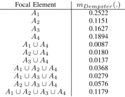
the combined bba, which is listed in Table II. TABLE II
FUSION OF4BBA’S WITHDEMPSTER’S RULE FORCOWA-ER.
Focal Element 𝑚𝐷𝑒𝑚𝑝𝑠𝑡𝑒𝑟(.) 𝐴1 0.2522 𝐴2 0.1151 𝐴3 0.1627 𝐴4 0.1894 𝐴1∪ 𝐴4 0.0087 𝐴2∪ 𝐴4 0.0180 𝐴3∪ 𝐴4 0.0137 𝐴1∪ 𝐴2∪ 𝐴4 0.0368 𝐴1∪ 𝐴3∪ 𝐴4 0.0279 𝐴2∪ 𝐴3∪ 𝐴4 0.0576 𝐴1∪ 𝐴2∪ 𝐴3∪ 𝐴4 0.1179
In step 4, we use Pignistic Transformation to obtain the bba’s corresponding pignistic probability listed in Table III. More efficient (but complex) transformations, like DSmP, could be used instead [19]. Based on the pignistic probability obtained, the decision result is 𝐴1.
TABLE III
PIGNISTICPROBABILITY BASED ONCOWA-ER.
Focal Element 𝐵𝑒𝑡𝑃 (.)
𝐴1 0.3076
𝐴2 0.1851
𝐴3 0.2275
𝐴4 0.2798
3) Implementation of FCOWA-ER: In step 1 of FCOWA-ER, we normalize each column in 𝐸[𝐶], respectively. In our example, one gets:
𝐸𝐹 𝑢𝑧𝑧𝑦[𝐶] = ⎡ ⎢ ⎣ [6.2/6.2; 10.9/13.2] [3.8/6.2; 11.4/13.2] [4.8/6.2; 11.2/13.2] [5.2/6.2; 13.2/13.2] ⎤ ⎥ ⎦ ≈ ⎡ ⎢ ⎣ [1.0000; 0.8258] [0.6129; 0.8636] [0.7742; 0.8485] [0.8387; 1.0000] ⎤ ⎥ ⎦ 3Other combination rules can be used instead to circumvent the limitations of Dempsters rule discuseed in [19], [20].
Then we obtain two FMFs, which are 𝜇1= [1, 0.6129, 0.7742, 0.8387];
𝜇2= [0.8258, 0.8636, 0.8485, 1.0000].
In step 2, by using𝛼-cut approach, 𝜇1and𝜇2are converted into two bba’s 𝑚𝑃 𝑒𝑠𝑠(.) and 𝑚𝑂𝑝𝑡𝑖(.) as listed in Table IV. In Step 3, we use Dempster’s rule4 to combine𝑚𝑃 𝑒𝑠𝑠(.) and
TABLE IV
THE TWO BBA’S TO COMBINE OBTAINED FROMFMFS.
Focal Element 𝑚𝑃 𝑒𝑠𝑠(.) Focal Element 𝑚𝑂𝑝𝑡𝑖(.)
𝐴1∪ 𝐴2∪ 𝐴3∪ 𝐴4 0.6129 𝐴1∪ 𝐴2∪ 𝐴3∪ 𝐴4 0.8257
𝐴1∪ 𝐴3∪ 𝐴4 0.1613 𝐴2∪ 𝐴3∪ 𝐴4 0.0227
𝐴1∪ 𝐴4 0.0645 𝐴2∪ 𝐴4 0.0152
𝐴1 0.1613 𝐴4 0.1364
𝑚𝑂𝑝𝑡𝑖(.) to get 𝑚𝐷𝑒𝑚𝑝𝑠𝑡𝑒𝑟(.) as listed in Table V.
TABLE V
FUSION OF TWO BBA’S WITHDEMPSTER’S RULE FORFCOWA-ER.
Focal Element 𝑚𝐷𝑒𝑚𝑝𝑠𝑡𝑒𝑟(.) 𝐴1 0.1370 𝐴4 0.1227 𝐴1∪ 𝐴4 0.0549 𝐴2∪ 𝐴4 0.0096 𝐴3∪ 𝐴4 0.0038 𝐴1∪ 𝐴3∪ 𝐴4 0.1370 𝐴2∪ 𝐴3∪ 𝐴4 0.0143 𝐴1∪ 𝐴2∪ 𝐴3∪ 𝐴4 0.5207
In step 4, we use again the Pignistic Transformation to get the pignistic probabilities listed in Table VI. Based on
TABLE VI
PIGNISTICPROBABILITY BASED ONFCOWA-ER.
Focal Element 𝐵𝑒𝑡𝑃 (.)
𝐴1 0.3403
𝐴2 0.1397
𝐴3 0.1826
𝐴4 0.3374
these probabilities, the decision result is also𝐴1. The decision results of COWA-ER and FCOWA-ER are the same.
IV. ANALYSES ONFCOWA-ER A. On computational complexity
In FCOWA-ER, only two bba’s are involved in the combi-nation. That is to say only one combination step is needed. Whereas in the original COWA-ER, if there exists 𝑞 alterna-tives, there should be𝑞 − 1 evidence combination operations to do. Furthermore, the bba’s obtained in the FCOWA-ER by using 𝛼-cut are consonant support (nested in order). This will bring less computational complexity when compared with the bba’s generated in the original COWA-ER. In summary, it is clear that the new proposed FCOWA-ER has lower computational complexity.
4In fact, and more generally the choice of a rule of combination is entirely left to the preference of the user in our FCOWA-ER methodology.
B. On physical meaning
In this new FCOWA-ER approach, the two different infor-mation sources are pessimistic OWA and optimistic OWA. The combination result can be regarded as a tradeoff between these two attitudes. the physical or practical meaning is relatively clear. Furthermore, if the decision-maker has preference on pessimistic or optimistic attitude, one can use discounting in evidence combination to satisfy one’s preference. We can set the preference of pessimistic attitude as 𝜆𝑝 and set the the preference of optimistic attitude as 𝜆𝑜. Then the discounting factor can be obtained as
{
𝛽 = 𝜆𝑜/𝜆𝑝, 𝜆𝑜≤ 𝜆𝑝
𝛽 = 𝜆𝑝/𝜆𝑜, 𝜆𝑝< 𝜆𝑜 (10)
Then according to the discounting method [16], one will take:
{
𝑚𝛽(𝑋) = 𝛽 ⋅ 𝑚(𝑋), for 𝑋 ∕= Θ
𝑚𝛽(Θ) = 𝛽 ⋅ 𝑚(Θ) + (1 − 𝛽) (11)
If 𝜆𝑜 ≤ 𝜆𝑝, then 𝑚(.) in (11) should be 𝑚𝑂𝑝𝑡𝑖(.); If 𝜆𝑝 ≤ 𝜆𝑜, then 𝑚(.) in (11) should be 𝑚𝑃 𝑒𝑠𝑠(.); By using
the discounting and choosing a combination rule, the decision maker’s has a flexibility in his decision-making process. C. On management of uncertainty
In the FCOWA-ER, we first define the bba vertically taking into account the uncertainty between alternatives for the pessimist attitude and for the optimistic attitude. Then we combine two columns. The uncertainty incorporated in the FMF obtained, which represents the possibility of each alternative to be chosen as the final decision result. Based on 𝛼-cut approach, the FMF is transformed into bba. The uncertainty is thus transformed to the bba. Although based on each column, only the information of pessimistic or optimistic is used, the combination operation followed can use both the two information sources (pessimistic and optimistic attitudes). Thus the available information can be fully used in FCOWA-ER. In COWA-ER, the modeling for each row (interval) takes into account the true uncertainty one has on the bounds of payoff for each alternative, then after modeling each bba 𝑚𝑖(.), one combines them ”vertically” to take into account
the uncertainty between alternatives.
Although the ways to manage the uncertainty incorporated in are different for COWA-ER and FCOWA-ER, they both utilize (differently) the whole available information.
D. On robustness to error scoring
Based on many experiments, we have observed that almost all the decision results given by FCOWA-ER agree5 with
COWA-ER results and are rational. However when the dif-ference among the values in payoff matrix is significant, the COWA-ER can yield to wrong decisions whereas FCOWA-ER yields to rational decisions as illustrated in Example 2 below. 5when using the same rule of combination in steps 3, and the same probabilistic transformation in steps 4.
Example 2Let’s take states 𝑆 = {𝑆1, 𝑆2, 𝑆3, 𝑆4, 𝑆5} with associated bba𝑚(𝑆1∪ 𝑆2∪ 𝑆3∪ 𝑆4∪ 𝑆5) = 1, and consider alternatives𝐴 = {𝐴1, 𝐴2, 𝐴3, 𝐴4} and the payoffs matrix:
𝐶 = ⎡ ⎢ ⎣ 12 11 10 120 7 9 10 6 110 3 7 13 5 100 6 6 2 3 150 4 ⎤ ⎥ ⎦ (12)
We see that the difference between max value and min value of each line is significant. For example, in the fourth row of 𝐶, only 𝑆4brings extremely high score for𝐴4 whereas other states bring homogeneous low score values for𝐴4. Whatever state of nature we consider𝑆1,𝑆2,. . . , or𝑆5,𝐴1 is either the top 1 or top 2 choice according to the ranks of the alternatives for states𝑆𝑖,𝑖 = 1, . . . , 5 as shown below:
𝐴1 𝐴2 𝐴3 𝐴4 𝑆1 1 2 3 4 𝑆2 2 3 1 4 𝑆3 1 2 3 4 𝑆4 2 3 4 1 𝑆5 1 4 2 3
So, intuitively, according to the principle of majority voting, the decision result should be 𝐴1 but not 𝐴4. According to rank-level fusion, the decision result should also be𝐴1.
The expected payoffs are:
𝐸[𝐶] = ⎡ ⎢ ⎣ [7, 120] [3, 110] [5, 100] [2, 150] ⎤ ⎥ ⎦ ∙ Using COWA-ER, one has
𝐸𝐼𝑚𝑝[𝐶] = ⎡ ⎢ ⎣ [0.0467, 0.8000] [0.0200, 0.7333] [0.0333, 0.6667] [0.0133, 1.0000] ⎤ ⎥ ⎦
The bba’s to combine are listed in Table VII and the combination results by using Dempster’s rule are in Table VIII.
TABLE VII
EXAMPLE2:BBA’S OF THE ALTERNATIVES USED INCOWA-ER.
Alternatives𝐴𝑖 𝑚𝑖(𝐴𝑖) 𝑚𝑖( ¯𝐴𝑖) 𝑚𝑖(𝐴𝑖∪ ¯𝐴𝑖)
𝐴1 0.0467 0.2000 0.7533
𝐴2 0.0200 0.2667 0.7133
𝐴3 0.0333 0.3333 0.6334
𝐴4 0.0133 0 0.9867
The pignistic probabilities listed in IX indicate that the decision result6 of COWA-ER is 𝐴
4.
∙ Using FCOWA-ER, one has 𝐸𝐹 𝑢𝑧𝑧𝑦[𝐶] = ⎡ ⎢ ⎣ [1.0000, 0.8000] [0.4286, 0.7333] [0.7143, 0.6667] [0.2857, 1.0000] ⎤ ⎥ ⎦
In FCOWA-ER, the bba’s to combine are listed in Table X and their Dempster’s combination is listed in Table XI.
TABLE VIII
EXAMPLE2: DEMPSTER’S FUSION OF4BBA’S FORCOWA-ER.
Focal Element 𝑚𝐷𝑒𝑚𝑝𝑠𝑡𝑒𝑟(.) 𝐴1 0.0438 𝐴2 0.0182 𝐴3 0.0309 𝐴4 0.0297 𝐴1∪ 𝐴4 0.0664 𝐴2∪ 𝐴4 0.0471 𝐴3∪ 𝐴4 0.0335 𝐴1∪ 𝐴2∪ 𝐴4 0.1775 𝐴1∪ 𝐴3∪ 𝐴4 0.1261 𝐴2∪ 𝐴3∪ 𝐴4 0.0895 𝐴1∪ 𝐴2∪ 𝐴3∪ 𝐴4 0.3373 TABLE IX
EXAMPLE2: PIGNISTICPROBABILITY BASED ONCOWA-ER.
Focal Element 𝐵𝑒𝑡𝑃 (.) 𝐴1 0.2625 𝐴2 0.2152 𝐴3 0.2038 𝐴4 0.3185 TABLE X
EXAMPLE2:BBA’S OF THE ALTERNATIVES USED INFCOWA-ER.
Focal Element 𝑚𝑃 𝑒𝑠𝑠(.) Focal Element 𝑚𝑂𝑝𝑡𝑖(.)
𝐴1∪ 𝐴2∪ 𝐴3∪ 𝐴4 0.2857 𝐴1∪ 𝐴2∪ 𝐴3∪ 𝐴4 0.6667
𝐴1∪ 𝐴2∪ 𝐴3 0.1429 𝐴1∪ 𝐴3∪ 𝐴4 0.0667
𝐴1∪ 𝐴3 0.2857 𝐴3∪ 𝐴4 0.0667
𝐴1 0.2857 𝐴1 0.1999
TABLE XI
EXAMPLE2: DEMPSTER’S FUSION OF THE TWO BBA’S FORFCOWA-ER.
Focal Element 𝑚𝐷𝑒𝑚𝑝𝑠𝑡𝑒𝑟(.) 𝐴1 0.3223 𝐴4 0.0667 𝐴1∪ 𝐴2 0.0111 𝐴1∪ 𝐴3 0.2222 𝐴1∪ 𝐴4 0.0222 𝐴1∪ 𝐴2∪ 𝐴3 0.1111 𝐴1∪ 𝐴2∪ 𝐴4 0.0222 𝐴1∪ 𝐴2∪ 𝐴3∪ 𝐴4 0.2222
The pignistic transformation of 𝑚𝐷𝑒𝑚𝑝𝑠𝑡𝑒𝑟(.) yields to the pignistic probabilities listed in Table XII.
TABLE XII
EXAMPLE2: PIGNISTIC PROBABILITY BASED ONFCOWA-ER.
Focal Element 𝐵𝑒𝑡𝑃 (.)
𝐴1 0.5500
𝐴2 0.1056
𝐴3 0.2037
𝐴4 0.1407
Based on the pignistic probabilities, the decision result obtained with FCOWA-ER is now 𝐴1, which is the correct one. In this example, FCOWA-ER shows its robustness when compared with COWA-ER.
E. On the normalization procedures
In fact, there exist at least three normalization procedures that we briefly recall below. Supposex is the original vector
6based on max of𝐵𝑒𝑡𝑃 (.).
input, xi represents the 𝑖th dimension of x. 𝑦𝑖 represents the 𝑖th dimension of the normalized vector y, then we examine the following three types of normalization:
1) Type I:𝑦𝑖= 𝑥𝑖/ max(x)
2) Type II:𝑦𝑖= (𝑥𝑖− min(x))/(max(x) − min(x)) 3) Type III:𝑦𝑖= 𝑥𝑖/∑𝑗(𝑥𝑗)
To verify wether the decision results of COWA-ER and the new FCOWA-ER can be affected by the normalization procedure, we did some tests as follows. We randomly generate payoff matrices and use all the three types of normalization approaches in COWA-ER and FCOWA-ER respectively. Then we make comparisons among the results obtained. We repeat the experiment 50 times (50 Monte-Carlo runs). Based on our simulation results, we find that normalization approaches can affect the decision results of COWA-ER and FCOWA-ER, although the ratio of disagreement among different normalization approach is small (about 1 to 2 times of disagreement out of 50 experiments in average). Example 3 is a case where the disagreement occurs due to the different types of normalization.
Example 3: We consider the following payoff matrix
𝐶 = ⎡ ⎢ ⎣ 15 5 30 5 40 40 40 30 30 15 10 40 ⎤ ⎥ ⎦ The bba is 𝑚(𝑋1) = 0.5439, 𝑚(𝑋2) = 0.3711, 𝑚(𝑋3) = 0.0849, where 𝑋1= 𝑆2∪ 𝑆3, 𝑋2 = 𝑆1∪ 𝑆2 and 𝑋3= 𝑆1∪ 𝑆3.
∙ Using COWA-ER, based on normalization Type I, Type II and Type III, we can obtain the corresponding expected payoffs 𝐸𝐼[𝐶] = [ [0.1462, 0.6108] [0.6009, 1.0000] [0.7500, 0.8640] [0.2606, 0.7680] ] 𝐸𝐼𝐼[𝐶] = [ [0.0000, 0.5442] [0.5326, 1.0000] [0.7072, 0.8407] [0.1340, 0.7283] ] 𝐸𝐼𝐼𝐼[𝐶] = [ [0.0292, 0.1221] [0.1202, 0.2000] [0.1500, 0.1728] [0.0521, 0.1536] ]
Then we obtain the pignistic probabilities listed in Table XIII. From Table XIII, one sees that the decision result with Type III normalization is 𝐴2 while those of Type I and Type II yields𝐴3.
TABLE XIII
EXAMPEL3: PIGNISTICPROB.FORTYPESI, II & IIIANDCOWA-ER.
Focal Element 𝐵𝑒𝑡𝑃𝐼(.) 𝐵𝑒𝑡𝑃𝐼𝐼(.) 𝐵𝑒𝑡𝑃𝐼𝐼𝐼(.)
𝐴1 0.0587 0.0388 0.1690
𝐴2 0.3203 0.3324 0.3180
𝐴3 0.5223 0.5444 0.2920
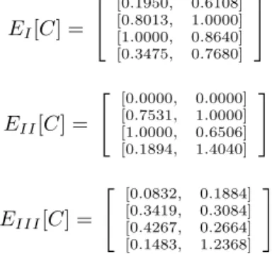
∙ Using FCOWA-ER, based on normalization of Type I, Type II and Type III, we get the corresponding expected payoffs 𝐸𝐼[𝐶] = [ [0.1950, 0.6108] [0.8013, 1.0000] [1.0000, 0.8640] [0.3475, 0.7680] ] 𝐸𝐼𝐼[𝐶] = [ [0.0000, 0.0000] [0.7531, 1.0000] [1.0000, 0.6506] [0.1894, 1.4040] ] 𝐸𝐼𝐼𝐼[𝐶] = [ [0.0832, 0.1884] [0.3419, 0.3084] [0.4267, 0.2664] [0.1483, 1.2368] ]
Then we can get the pignistic probabilities listed in Table XIV. From Table XIV, one sees that the decision with Type II normalization is𝐴2 while those of Type I and Type III yields 𝐴3.
TABLE XIV
EXAMPLE3: PIGNISTIC PROBABILITY BASED ONFCOWA-ER
Focal Element 𝐵𝑒𝑡𝑃𝐼(.) 𝐵𝑒𝑡𝑃𝐼𝐼(.) 𝐵𝑒𝑡𝑃𝐼𝐼𝐼(.)
𝐴1 0.0306 0.0000 0.0306
𝐴2 0.4118 0.5421 0.4118
𝐴3 0.4763 0.4300 0.4763
𝐴4 0.0813 0.0279 0.0813
So in a little percentage of cases, we must be cautious when choosing a normalization procedure and so far there is no clear theoretical answer for the choice of the most adapted normalization procedure. We prefer the Type I normalization procedure since it is very simple and intuitively appealing.
V. CONCLUSION
In this paper, we have proposed a fuzzy cautious OWA method using evidential reasoning (FCOWA-ER) to implement the multi-criteria decision making, where evidence theory, fuzzy membership functions and OWA are used jointly. This method has less computational complexity and has clearer physical meaning. Furthermore, it is more robust to the error scoring in MCDM. Experimental results and related analyses show that our FCOWA-ER is interesting and flexible because its three main specifications can be adapted easily for working: 1) with other rules of combination than Dempster’s rule, 2) with other probabilistic transformations than BetP, and 3) with different normalization procedures. Of course the performances of FCOWA-ER depend on the choice of these three main specifications taken by the MCDM system designer. The method to generate the bba from the FMF based on 𝛼-cut depends on the selection of the parameter vector of 𝛼. The impact of the choice of the specifications as well as 𝛼 to evaluate the performance of FCOWA-ER will be further analyzed in our future works. This paper was devoted to the theoretical developemnt of FCOWA-ER and its evaluation for applications to real MCDM problems is part of our future research works.
ACKNOWLEDGMENT
This work is supported by National Natural Science Foun-dation of China (No.61104214, No.67114022, No. 61074176, No. 60904099), Fundamental Research Funds for the Cen-tral Universities, China Postdoctoral Science Foundation (No.20100481337, No.201104670), Research Fund of Shaanxi Key Laboratory of Electronic Information System Integration (No.201101Y17), Chongqing Natural Science Foundation (No. CSCT, 2010BA2003) and Aviation Science Foundation (No. 2011ZC53041).
REFERENCES
[1] B. Roy, “Paradigms and challenges”, in Multiple Criteria Decision Analysis : State of the art surveys, Vol.78 of Int. Series in Oper. Research and& Management Sci. (Chap. 1), pp. 1–24, Springer, 2005.
[2] R. Yager, “On ordered weighted averaging operators in multi-criteria decision making”, IEEE Transactions on Systems, Man and Cybernetics, 18:183–190, 1988.
[3] R. Yager, J. Kacprzyk, The ordered weighted averaging operator: theory
and applications, Kluwer Academic Publishers, MA: Boston, 1997.
[4] M. O’Hagan, “Aggregating template rule antecedents in real-time expert systems with fuzzy set logic”, Proc. of 22nd Ann. IEEE Asilomar Conf. on Signals, Systems and Computers, Pacific Grove, CA, 1988, 681–689. [5] D. Filev, R. Yager, “On the issue of obtaining OWA operator weights”,
Fuzzy Sets and Systems, 94: 157–169, 1998.
[6] B.S. Ahn, “Parameterized OWA operator weights: an extreme point approach”, International Journal of Approximate Reasoning, 51: 820– 831, 2010.
[7] R. Yager, “Using stress functions to obtain OWA operators”, IEEE
Transactions on Fuzzy Systems, 15: 1122C-1129, 2007.
[8] Y.M. Wang, C. Parkan, “A minimax disparity approach obtaining OWA operator weights”, Information Sciences, 175: 20–29, 2005.
[9] A. Emrouznejad, G.R. Amin, “Improving minimax disparity model to determine the OWA operator weights”, Information Sciences, 180: 1477– 1485, 2010.
[10] Y.M. Wang, Y. Luo, Z. Hua, “Aggregating preference rankings using OWA operator weights”, Information Sciences 177: 3356–3363, 2007. [11] M. Beynon, “A method of aggregation in DS/AHP for group
decision-making with non-equivalent importance of individuals in the group”,
Computers and Operations Research, 32: 1881–1896, 2005.
[12] J. Dezert, J.-M. Tacnet, M. Batton-Hubert, F. Smarandache,“Multi-criteria decision making based on DSmT-AHP”, Proc. of Belief 2010 Int. Workshop, Brest, France, 1-2 April, 2010.
[13] J.-M. Tacnet, M. Batton-Hubert, J. Dezert, “A two-step fusion process for multi-criteria decision applied to natural hazards in mountains”, Proc. of Belief 2010 Int. Workshop, Brest, France, 2010.
[14] R. Yager, “Decision making under Dempster-Shafer uncertainties”, Studies in Fuzziness and Soft Computing, 219:619–632, 2008. [15] J.-M. Tacnet, J. Dezert, “ Cautious OWA and evidential reasoning
for decision making under uncertainty”, Proc. of 14th International Conference on Information Fusion Chicago, Illinois, USA, July 5-8, 2011, 2074–2081.
[16] G. Shafer, A Mathematical Theory of Evidence, Princeton University, Princeton, 1976.
[17] J. Dezert,“Autonomous navigation with uncertain reference points using the PDAF”, Multitarget-Multisensor Tracking, Vol 2, pp 271–324, Y. Bar-Shalom Editor, Artech House, 1991.
[18] M. C. Florea, A.-L. Jousselme, D. Grenier, ´E. Boss´e, “Approximation techniques for the transformation of fuzzy sets into random sets”, Fuzzy
Sets and Systems, 159: 270–288, 2008.
[19] F. Smarandache, J. Dezert, “Advances and applications of DSmT for in-formation fusion (Collected works)”, Vol. 1-3, American Research Press, 2004–2009.http://www.gallup.unm.edu/˜smarandache/DSmT.htm
[20] J. Dezert, P. Wang, A. Tchamova, “On the validity of Dempster-Shafer Theory”, in Proceedings of Fusion 2012 Conf., Singapore, July 2012.