Reynolds-Averaged Navier-Stokes Based Ice Accretion For Aircraft Wings

(1)

UNIVERSITÉ DE MONTRÉAL

REYNOLDS-AVERAGED NAVIER-STOKES BASED ICE ACCRETION FOR

AIRCRAFT WINGS

KAZEM HASANZADEH LASHKAJANI DÉPARTEMENT DE GÉNIE MÉCANIQUE ÉCOLE POLYTECHNIQUE DE MONTRÉAL

THÈSE PRÉSENTÉE EN VUE DE L’OBTENTION DU DIPLÔME DE PHILOSOPHIAE DOCTOR

(GÉNIE MÉCANIQUE) DÉCEMBRE 2015

(2)

UNIVERSITÉ DE MONTRÉAL

ÉCOLE POLYTECHNIQUE DE MONTRÉAL

Cette thèse intitulée :

REYNOLDS-AVERAGED NAVIER-STOKES BASED ICE ACCRETION FOR

AIRCRAFT WINGS

présentée par : HASANZADEH LASHKAJANI Kazem en vue de l’obtention du diplôme de : Philosophiae Doctor a été dûment acceptée par le jury d’examen constitué de :

M. TRÉPANIER Jean-Yves, Ph.D., président

M. PARASCHIVOIU Ion, Doctorat, membre et directeur de recherche M. LAURENDEAU Eric, Ph.D., membre et codirecteur de recherche M. CAMARERO Ricardo, Ph.D., membre

(3)

DEDICATION

(4)

ACKNOWLEDGEMENTS

The work has been performed through a Collaborative R&D Grant No. 341083–06 with Bombardier Aerospace and the Natural Sciences and Engineering Research Council of Canada (NSERC).

First, I would like to express my gratitude to my research directors, Professor Eric Laurendeau and Professor Ion Paraschivoiu for their support of my Ph. D. study.

Particularly, I would like to express my sincere appreciation to Professor Eric Laurendeau, for his patience, knowledge, motivation and guidance through the entire course of my research study. An outstanding teacher, who has taught me the insight in fluid mechanical engineering and its industrial applications.

I would like to thank Dr. Sina Arabi, my friend, who has helped me to understand the knowledge of mesh generation.

An appreciation to BBA, advance aero department, especially to Mr. Corentin Brette, Dr. Patrick Germain, Dr. Alberto Pueyo, Dr. Guy Fortin, Dr. Kurt Sermeus, Mrs. Sherry Vafa for their help and support.

And at last, I would like to thank my friends and colleagues for the happy moments we spent during the study at Polytechnique Montreal.

(5)

RÉSUMÉ

Cette thèse aborde l'un des enjeux actuels de la sécurité aérienne pour augmenter les capacités de simulation de givrage pour la prédiction des formes complexes 2D et 3D de verglas sur les surfaces des aéronefs. Durant les années 1980 et 1990, le domaine de l'aérogivrage numérique s’est développé pour soutenir la conception et la certification des aéronefs volant dans des conditions givrantes. Les technologies multidisciplinaires utilisées dans ces codes étaient : l'aérodynamique (méthode des panneaux), le calcul des trajectoires des gouttelettes (méthode Lagrangienne), le module thermodynamique (modèle Messinger) et le module de géométrie (accumulation de glace). Ceux-ci sont intégrés dans un module quasi-stationnaire pour simuler le processus d'accumulation de glace en fonction du temps (procédure à plusieurs pas de temps). Les objectifs de la présente recherche visent à améliorer le module aérodynamique en passant de Laplace à un solveur d’équations de Navier-Stokes moyennée (RANS). Les avantages sont nombreux. Tout d'abord, le modèle physique permet le calcul des effets visqueux dans le module aérodynamique. Deuxièmement, la solution du programme d’aérogivrage fournit directement les moyens pour caractériser les effets aérodynamiques du givrage, comme la perte de portance et la traînée accrue. Troisièmement, l'utilisation d'une approche de volumes finis pour résoudre les équations aux dérivées partielles (PDE) permet des analyses rigoureuses de convergence en maillage et en temps. Enfin, les approches développées en 2D peuvent être facilement transposées aux problèmes 3D.

La recherche a été réalisée en trois étapes principales, chacune fournissant des aperçus des approches numériques globales. La réalisation la plus importante vient de la nécessité de développer des algorithmes de génération de maillage spécifiquement pour assurer des solutions réalisables en plusieurs étapes de calculs très complexes d’aéro-givrage. Les contributions sont présentées dans l’ordre chronologique de leurs réalisations.

D'abord, un nouveau cadre de simulation de glace bidimensionnel basé sur un code RANS, CANICE2D-NS, est développé. Un code RANS à maillage à simple bloc de l’université de Liverpool (nommé SMB) fournit la solution aérodynamique en utilisant le modèle de turbulence Spalart-Allmaras. L'outil commercial ICEM CFD est utilisé pour le remaillage du profil glacé pour le lissage du domaine. Le nouveau couplage est entièrement automatisé et capable d’effectuer des simulations d’accumulation de la glace à plusieurs pas de temps par une

(6)

approche quasi-stationnaire. En outre, le logiciel permet une analyse de l’écoulement de l’air et la prévision des performances aérodynamiques des profils glacés. La convergence de l'algorithme quasi-stationnaire est vérifiée et identifie la nécessité de l’augmentation d'un ordre de grandeur dans le nombre de pas de temps dans les simulations de givrage afin de parvenir à des solutions indépendantes du nombre d’incréments de temps.

Deuxièmement, un code Navier-Stokes à maillages à blocs multiples, NSMB, est couplé avec le programme de givrage CANICE2D. L’attention est accordée à l’implémentation du modèle de rugosité ONERA dans le modèle de turbulence Spalart-Allmaras et à la convergence de la procédure itérative stationnaire et quasi-stationnaire. Les effets d’une rugosité de surface uniforme dans la simulation quasi-stationnaire de l'accumulation de glace sont analysés à travers différents cas de validation. Les résultats de CANICE2D-NS montrent un bon accord avec les données expérimentales à la fois en termes de formes de glace prédites ainsi qu’en termes d’analyses aérodynamiques des formes de glace prédites et expérimentales.

Troisièmement, un code Navier-Stokes structuré à maillage à simple bloc, NSCODE, est couplé avec le cadre de givrage CANICE2D-NS. L’attention est accordée à l’implémentation de la rugosité du modèle Boeing dans le modèle de turbulence Spalart-Allmaras, et à l'accélération de la convergence des procédures itératives stationnaires et quasi-stationnaires. Les effets d’une rugosité de surface uniforme dans la simulation de l'accumulation quasi-stationnaire de glace sont analysés à travers différents cas de validation et de comparaisons entre codes avec le même programme couplé avec le solveur Navier-Stokes NSMB. L'efficacité de l'approche à grilles multiples dans la direction J est démontrée pour la résolution des équations d'écoulement d’air sur des géométries glacées complexes.

Puisqu’il a été remarqué à travers les différents résultats obtenus que le logiciel de génération de maillage ICEM-CFD produit un certain nombre de problèmes tels que la mauvaise qualité des maillages et les carences en lissage (notamment les chocs de mailles), une quatrième étude propose un nouvel algorithme de génération de maillages. Un code de génération de maillages en plusieurs blocs et basé sur la résolution d’équations aux dérivées partielles, NSGRID, est développé à cet effet. L'étude comprend les développements de nouveaux algorithmes de génération de maillage sur des formes complexes de verglas contenant des géométries d’accumulation de glace à courbure hautement variable, comme des cornes de glace

(7)

simples ou doubles. Une approche en deux étapes consiste à discrétiser la surface de la géométrie, puis le domaine de résolution. Un algorithme curviligne adaptatif contrôlant la courbure est construit en résolvant une équation elliptique 1D avec termes sources périodiques. Cette méthode contrôle l'espacement de la longueur d’arc des mailles sur la surface de telle sorte que les régions de forte courbure convexe et concave autour des cornes de glace sont captées de manière appropriée. Il est montré que cette méthode traite efficacement le problème de choc de mailles. Ensuite, une nouvelle méthode mixte est développée en définissant des combinaisons de termes sources avec des équations elliptiques 2D. Les termes sources comprennent deux fonctions de contrôle communes, Sorenson et Spekreijse, et un troisième terme source supplémentaire pour forcer l’orthogonalité. Cette méthode mixte s’avère être très efficace pour améliorer la qualité des mailles d’un maillage complexe de verglas avec une résolution RANS. La performance en termes de réduction des résidus par itérations non linéaires de plusieurs algorithmes de résolution (Point-Jacobi, Gauss-Seidel, ADI, Point et Line SOR) est discutée dans le contexte d'un opérateur multi grilles complet. Des détails sont donnés sur les différentes formulations utilisées dans le procédé de linéarisation. Il est montré que la performance de l'algorithme de solution dépend de la nature de la fonction de contrôle utilisée. Enfin, les algorithmes sont validés sur des formes de glace expérimentales standards et complexes, démontrant l'applicabilité des méthodes.

Finalement, un programme bidimensionnel de simulation d’accumulation de glace basé sur la résolution RANS et automatisé pour le calcul par plusieurs incréments de temps, CANICE2D-NS, est développé et couplé avec un code CFD Navier-Stokes multi blocs, NSCODE2D, un code de génération elliptique de maillages multi blocs, NSGRID2D, et un solveur multi blocs Eulérien pour la trajectoire des gouttelettes, NSDROP2D (développé à l'École Polytechnique de Montréal). Le programme permet des calculs Lagrangiens et Eulériens de trajectoires de gouttelettes, la dernière profitant d’une approche de maillages superposés pour traiter les géométries à éléments multiples. Le code a été testé sur des cas de validation confidentiels et publics, y compris les cas standards NATO. En outre, une accélération d’un facteur allant jusqu’à 10 est observée dans la procédure de génération de maillages en utilisant un lisseur implicite avec une procédure à grilles multiples. Les résultats démontrent les avantages et la robustesse du nouveau programme dans la prédiction des formes de glace et des paramètres de performances aérodynamique.

(8)

ABSTRACT

This thesis addresses one of the current issues in flight safety towards increasing icing simulation capabilities for prediction of complex 2D and 3D glaze ice shapes over aircraft surfaces. During the 1980’s and 1990’s, the field of aero-icing was established to support design and certification of aircraft flying in icing conditions. The multidisciplinary technologies used in such codes were: aerodynamics (panel method), droplet trajectory calculations (Lagrangian framework), thermodynamic module (Messinger model) and geometry module (ice accretion). These are embedded in a quasi-steady module to simulate the time-dependent ice accretion process (multi-step procedure). The objectives of the present research are to upgrade the aerodynamic module from Laplace to Reynolds-Average Navier-Stokes equations solver. The advantages are many. First, the physical model allows accounting for viscous effects in the aerodynamic module. Second, the solution of the aero-icing module directly provides the means for characterizing the aerodynamic effects of icing, such as loss of lift and increased drag. Third, the use of a finite volume approach to solving the Partial Differential Equations allows rigorous mesh and time convergence analysis. Finally, the approaches developed in 2D can be easily transposed to 3D problems.

The research was performed in three major steps, each providing insights into the overall numerical approaches. The most important realization comes from the need to develop specific mesh generation algorithms to ensure feasible solutions in very complex multi-step aero-icing calculations. The contributions are presented in chronological order of their realization.

First, a new framework for RANS based two-dimensional ice accretion code, CANICE2D-NS, is developed. A multi-block RANS code from U. of Liverpool (named PMB) is providing the aerodynamic field using the Spalart-Allmaras turbulence model. The ICEM-CFD commercial tool is used for the iced airfoil remeshing and field smoothing. The new coupling is fully automated and capable of multi-step ice accretion simulations via a quasi-steady approach. In addition, the framework allows for flow analysis and aerodynamic performance prediction of the iced airfoils. The convergence of the quasi-steady algorithm is verified and identifies the need for an order of magnitude increase in the number of multi-time steps in icing simulations to achieve solver independent solutions.

(9)

Second, a Multi-Block Navier-Stokes code, NSMB, is coupled with the CANICE2D icing framework. Attention is paid to the roughness implementation of the ONERA roughness model within the Spalart-Allmaras turbulence model, and to the convergence of the steady and quasi-steady iterative procedure. Effects of uniform surface roughness in quasi-quasi-steady ice accretion simulation are analyzed through different validation test cases. The results of CANICE2D-NS show good agreement with experimental data both in terms of predicted ice shapes as well as aerodynamic analysis of predicted and experimental ice shapes.

Third, an efficient single-block structured Navier-Stokes CFD code, NSCODE, is coupled with the CANICE2D-NS icing framework. Attention is paid to the roughness implementation of the Boeing model within the Spalart-Allmaras turbulence model, and to acceleration of the convergence of the steady and quasi-steady iterative procedures. Effects of uniform surface roughness in quasi-steady ice accretion simulation are analyzed through different validation test cases, including code to code comparisons with the same framework coupled with the NSMB Navier-Stokes solver. The efficiency of the J-multigrid approach to solve the flow equations on complex iced geometries is demonstrated.

Since it was noted in all these calculations that the ICEM-CFD grid generation package produced a number of issues such as inefficient mesh quality and smoothing deficiencies (notably grid shocks), a fourth study proposes a new mesh generation algorithm. A PDE based multi-block structured grid generation code, NSGRID, is developed for this purpose. The study includes the developments of novel mesh generation algorithms over complex glaze ice shapes containing multi-curvature ice accretion geometries, such as single/double ice horns. The twofold approaches tackle surface geometry discretization as well as field mesh generation. An adaptive curvilinear curvature control algorithm is constructed solving a 1D elliptic PDE equation with periodic source terms. This method controls the arclength grid spacing so that high convex and concave curvature regions around ice horns are appropriately captured and is shown to effectively treat the grid shock problem. Then, a novel blended method is developed by defining combinations of source terms with 2D elliptic equations. The source terms include two common control functions, Sorenson and Spekreijse, and an additional third source term to improve orthogonality. This blended method is shown to be very effective for improving grid quality metrics for complex glaze ice meshes with RANS resolution. The performance in terms of residual reduction per non-linear iteration of several solution algorithms (Point-Jacobi,

(10)

Gauss-Seidel, ADI, Point and Line SOR) are discussed within the context of a full Multi-grid operator. Details are given on the various formulations used in the linearization process. It is shown that the performance of the solution algorithm depends on the type of control function used. Finally, the algorithms are validated on standard complex experimental ice shapes, demonstrating the applicability of the methods.

Finally, the automated framework of RANS based two-dimensional multi-step ice accretion, CANICE2D-NS is developed, coupled with a Multi-Block Navier-Stokes CFD code, NSCODE2D, a Multi-Block elliptic grid generation code, NSGRID2D, and a Multi-Block Eulerian droplet solver, NSDROP2D (developed at Polytechnique Montreal). The framework allows Lagrangian and Eulerian droplet computations within a chimera approach treating multi-elements geometries. The code was tested on public and confidential validation test cases including standard NATO cases. In addition, up to 10 times speedup is observed in the mesh generation procedure by using the implicit line SOR and ADI smoothers within a multigrid procedure. The results demonstrate the benefits and robustness of the new framework in predicting ice shapes and aerodynamic performance parameters.

(11)

LIST OF TABLES

Table 1.1: Icing codes info ... 3

Table 1.2: PM icing codes info ... 9

Table 2.1: RANS solvers roughness models info ... 54

Table 4.1: NACA0012 run 405 test conditions ... 74

Table 4.2: NACA0012 run 408 test conditions ... 78

Table 6.1: NATO cases test conditions ... 125

Table 6.2: NATO cases failed test runs ... 134

(16)

LIST OF FIGURES

Figure 1.1: Rime and glaze ice shapes [2] ... 2

Figure 1.2: CANICE2D results and comparison for NATO/RTO exercise case studies [9] ... 3

Figure 1.3: Grid generated (rime ice [left] and glaze ice [right]) [12] ... 6

Figure 1.4: FENSAP-ICE 3D ice solution [14]. ... 7

Figure 2.1: CANICE code structure [2]. ... 12

Figure 2.2: Reference system definition for droplet trajectory calculation [49]. ... 23

Figure 2.3: Definition of the local and global collection efficiency [2]. ... 25

Figure 2.4: Surface control volume for mass and energy balance [5]. ... 27

Figure 2.5: Grids generated with ICEM-CFD [31, 39] ... 29

Figure 2.6: Mesh generated using GRIDGEN, elliptic (left), hyperbolic (right) [75]. ... 30

Figure 2.7: Grid generated for a glaze ice shape: (a) Single-block. (b) Multi-block [77]. ... 31

Figure 2.8: Grid generated and modified for glaze ice shape: (a) Grid line cluster next to the wall propagates into the domain along the block boundaries, (b) Effect of wrap-around to remove the clustering via the multi-block decomposition [77]. ... 31

Figure 2.9: Grid generated and modified for a glaze ice shape: (a) Surface oscillation is propagated into domain, (b) Transition layer removed the surface oscillation propagation [75]. ... 32

Figure 2.10: Grid generated and modified for a glaze ice shape with Turbo-Grid [78]. ... 32

Figure 2.11: Structured grid generated for two glaze ice shapes [12, 58]. ... 33

Figure 2.12: Deletion/insertion algorithm in two dimensional grids [79]. ... 36

Figure 2.13: Semi-structured grids for arbitrary 2D and 3D geometries [79, 80]. ... 37

Figure 2.14: Structured grid (left) and Semi-structured grid (right), 2D glaze ice shapes [79, 80]. ... 37

(17)

Figure 2.15: Grid generated without curvature effect (left), and with curvature effect (right) [56].

... 39

Figure 2.16: GRAPE generated mesh [55]. ... 42

Figure 2.17: Composite mapping [84]. ... 42

Figure 2.18: ENGRID generated mesh [22]. ... 43

Figure 2.19: Mesh around an iced airfoil, algebraic (left) and elliptic smoothing (right). ... 47

Figure 2.20: Grid spacing changes (curvature undesirable effects of Laplacian operators) [56]. . 47

Figure 2.21: Mapping for O-type (up) and C-type (down) mesh around an airfoil [55]. ... 48

Figure 2.22: Area weighted interpolation for 3 points. ... 55

Figure 4.1: CANICE code structure. ... 62

Figure 4.2: CANICE2D results and comparison for NATO/RTO exercise case studies [9]. ... 64

Figure 4.3: Mesh around ice shape, algebraic (left) and elliptic smoothing (right). ... 68

Figure 4.4: Flat plate grid. ... 69

Figure 4.5: Residual convergence, flat plate test case ... 69

Figure 4.6: Turbulent flat plate skin friction comparison: NSMB (SA-ONERA) with semi-empirical relation. ... 70

Figure 4.7: NACA0012 N-S grids ... 71

Figure 4.8: Residual Convergence, NACA0012 test case. ... 71

Figure 4.9: CL-Alpha graph for NACA0012 smooth and rough surface. ... 71

Figure 4.10: RAE2822 N-S grids. ... 72

Figure 4.11: Residual convergence, RAE2822 test case. ... 72

Figure 4.12: Pressure coefficients comparison for the case RAE2822. ... 73

Figure 4.13: Collection efficiency comparison (NACA0012 run 405).. ... 75

Figure 4.14: Effect of increased roughness on ice shape using CANICE2D-NS (NACA0012 run 405).. ... 75

(18)

Figure 4.15: Ice shape comparison for different roughness, CANICE2D-NS (NACA0012 run

405). ... 75

Figure 4.16: Ice shape comparison (NACA0012 run 405).. ... 76

Figure 4.17: NACA0012 run 405: C-mesh using automated ICEM grid generation for CANICE2D-NS multi-time step run. ... 76

Figure 4.18: NSMB convergence for 4 time-steps of CANICE2D-NS (case 405).. ... 77

Figure 4.19: Collection efficiency comparison (NACA0012 run 408).. ... 78

Figure 4.20: Effect of increase in roughness on ice shape using CANICE2D-NS (NACA0012 run 408). ... 79

Figure 4.21: Ice shape comparison for different roughness value, CANICE2D-NS (NACA0012 run 408).. ... 79

Figure 4.22: Ice shape comparison for NACA0012 run 408.. ... 80

Figure 4.23: NACA0012 run 408 C-mesh using automated ICEM grid generation for CANICE2D-NS multi-time step run.. ... 80

Figure 4.24: NSMB convergence for 5 time-steps of CANICE2D-NS (case 408).. ... 80

Figure 4.25: ICEM mesh generated experimental ice shape (case 405). ... 82

Figure 4.26: CL comparison (case 405).. ... 82

Figure 4.27: Pressure coefficient comparison (α=6o, case 405). (Right, leading edge zoom).. ... 82

Figure 4.28: ICEM mesh generated for experimental ice shape (case 408).. ... 83

Figure 4.29: CL comparison (case 408).. ... 84

Figure 4.30: Pressure coefficient comparison (α=6o, case 408). (Right, leading edge zoom).. ... 84

Figure 4.31: NACA0012 run 405 ice shape comparison with increasing time steps (CANICE2D-NS).. ... 85

Figure 4.32: NACA0012 run 405 ice shape comparison with increasing time steps (CANICE2D-Panel Method). ... 85

(19)

Figure 4.33: NACA0012 run 408 ice shape comparison with increasing time steps

(CANICE2D-NS).. ... 86

Figure 4.34: NACA0012 run 408 ice shape comparison with increasing time steps (CANICE2D-Panel Method).. ... 86

Figure 4.35: RMS comparison for the multi-time steps ice shape convergence (cases 405 and 408).. ... 87

Figure 5.1: Simple mapping: Computational space (left), Physical space (right).. ... 94

Figure 5.2: Composite mapping: Computational space (left), Parametric space (middle), Physical space (right).. ... 96

Figure 5.3: Computed curvature (left axis: geometry curvature in red, selected points in green); Curvature based distributed points spacing along the wall (right axis: for different coefficient A).. ... 100

Figure 5.4: Parabolic grid generated for 1D PDE geometry points distribution for two different coefficients A: 2.5×10-4_{, left, and 1×10}-3_{, right. ... 101}

Figure 5.5: 1D PDE Curvature based point distribution for different coefficient A with Point SOR (PS) and ADI. ... 101

Figure 5.6: Algebraic grid. ... 102

Figure 5.7: Parabolic grid. ... 102

Figure 5.8: Poisson elliptic grid with no source terms. ... 102

Figure 5.9: Elliptic grid with RLS source terms ... 103

Figure 5.10: Elliptic grid with SPS source terms. ... 103

Figure 5.11: Computed curvature (left axis: geometry curvature in red, selected points in green); Curvature based distributed points spacing along the wall (right axis: for coefficient A=8×10-4).. ... 103

Figure 5.12: Elliptic grid comparison for different right hand side source term: RLS (top left), RLS-SPS (top right), and RLS-SPS-Para (bottom).. ... 104

(20)

Figure 5.13: Algebraic grid (top left) and its parametric space (bottom left); Parabolic grid (top

right) and its parametric space (bottom right).. ... 105

Figure 5.14: NSGRID solution convergence for different blended source terms. ... 105

Figure 5.15: Minimum grid spacing close to wall. ... 106

Figure 5.16: Grid selected indexes, I (148) and J (50) to compute and compare the grid quality criteria. ... 107

Figure 5.17: Grid quality comparison on i=148 (for (1≤ j ≤50): Orthogonality (left), Skewness (right).. ... 107

Figure 5.18: J Stretch Ratio comparison on i=148 (for (1≤ j ≤50).. ... 108

Figure 5.19: I Stretch Ratio comparison on j =50 (for 1≤ i ≤257).. ... 108

Figure 5.20: Solver comparison on the elliptic equation with blended source term (RLS-SPS-Para).. ... 109

Figure 5.21: Multi-grid effects comparison on ADI-I and LS-I. ... 109

Figure 5.22: Linearization comparison, NR and SS, on ADI-I. ... 110

Figure 5.23: Elliptic grid generated with blended approach RLS-SPS-Para. ... 111

Figure 5.24: Grid solution convergence of the blended source term (RLS-SPS-Para), using LS-I, with 2 levels of Multi-Grid. ... 112

Figure 5.25: Lift coefficient versus angle of attack. ... 112

Figure 5.26: Drag coefficient versus angle of attack. ... 113

Figure 5.27: NSCODE flow convergence comparison for AOA of 0°.. ... 113

Figure 5.28: Elliptic grid generated with blended approach RLS-SPS-Para. ... 114

Figure 5.29: Computed curvature (left axis: geometry curvature in red, selected points in green); Curvature based distributed points spacing along the wall (right axis: for coefficient A=2×10-4).. ... 114

Figure 5.30: Grid solution convergence of the blended source term (RLS-SPS-Para), using LS-I, with 2 levels of Multi-Grid. ... 115

(21)

Figure 5.31: Lift coefficient versus angle of attack ... 115

Figure 5.32: Drag coefficient versus angle of attack. ... 115

Figure 5.33: Cp comparison for AOA of 0°.. ... 116

Figure 5.34: NSCODE flow convergence comparison for AOA of 0°.. ... 116

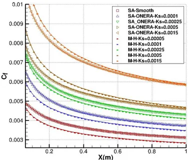
Figure 6.1: Turbulent flat plate skin friction comparison: NSCODE (SA-Boeing) with semi-empirical relation ... 119

Figure 6.2: Residual Convergence, NSMB and NSCODE on the RAE2822 airfoil ... 120

Figure 6.3: Pressure coefficients comparison for the RAE2822 airfoil ... 120

Figure 6.4: NACA0012 run 408 glaze ice C-mesh using automated ICEM grid generation ... 121

Figure 6.5: Convergence rates comparison of SG, FMG, and FMG-J. ... 121

Figure 6.6: Collection efficiency comparison. ... 122

Figure 6.7: Ice shape comparison for different roughness, CANICE2D-NSCODE, run 405 (left), run 408 (right). ... 122

Figure 6.8: Ice shape comparison with literature data, CANICE2D-NSCODE, run 405 (left), run 408 (right). ... 123

Figure 6.9: Multi-steps convergence of CANICE2D-NSBM compared to CANICE2D-NSCODE, run 405 (left), run 408 (right). ... 123

Figure 6.10: Convergence rate, NSGRID2D (left), NSCODE2D flow (right), (case C09, TS=5) ... 125

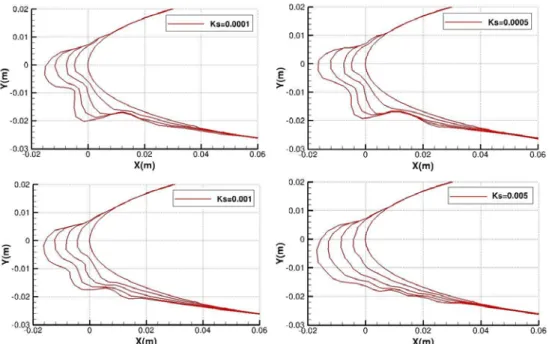
Figure 6.11: Ice shape formation effected by roughness for case with 5 time steps: case C09 rime ice (top), case C17 glaze ice (down); Ks =0.0001 (left), Ks =0.0005 (middle), Ks =0.001 (right).. ... 126

Figure 6.12: Collection efficiency comparison: Lagrangian method, top-left; Ice shape comparison: (Ks=0.0001), top-right; (Ks=0.0005), down-left; (Ks=0.001), down-right .... 126

(22)

Figure 6.14: Collection efficiency comparison: Lagrangian method, top-left; Ice shape comparison: (Ks=0.0001), top-right; (Ks=0.0005), down-left; (Ks=0.001), down-right... . 127

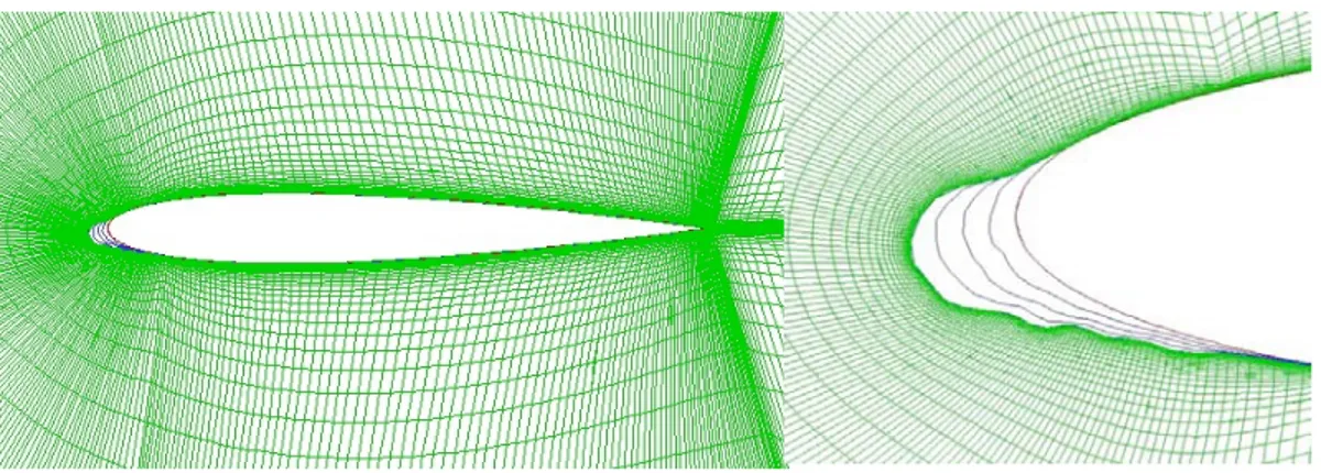
Figure 6.15: Generated grid and computed flow, (TS=5, Ks=0.001, case C17)... ... 127

Figure 6.16: Collection efficiency comparison: Lagrangian method, top-left; Ice shape comparison: (Ks=0.0001), top-right; (Ks=0.0005), down-left; (Ks=0.001), down-right. ... 128

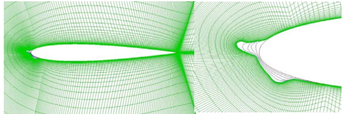
Figure 6.17: Generated grid and computed flow, (TS=5, Ks=0.001, case C10). ... 128

Figure 6.18: Collection efficiency comparison: Lagrangian method, top-left; Ice shape comparison: (Ks=0.0001), top-right; (Ks=0.0005), down-left; (Ks=0.001), down-right. ... 129 Figure 6.19: Generated grid and computed flow, (TS=5, Ks=0.001, case C13).. ... 129

Figure 6.23: Generated grid and computed flow, (TS=5, Ks=0.001, case C18).. ... 131

Figure 6.24: Ice shape comparison: (Ks=0.0001), left; (Ks=0.001), right. ... 132

Figure 6.26: Ice shape comparison: (Ks=0.0001), left; (Ks=0.001), right. ... 132

(23)

LIST OF SYMBOLS AND ABBREVIATIONS

Lift coefficient Drag coefficient Skin friction coefficient Pressure coefficient

AOA Angle of attack

LWC Liquid water content (kg/m3)

MED Mean droplet diameter (m)

w Wall value

Transported quantity in the S-A model Distance to the nearest wall (m)

Offset in the wall distance to account for wall roughness (m)

Equivalent sand grain roughness height (m)

Equivalent sand grain roughness height normalized by chord Von Karman constant

Transformed vorticity

Distance along the wall normal (m) Normalized wall distance /

Longitudinal velocity component (m/s) Turbulent eddy viscosity (m2/s)

Friction velocity (m/s)

, Turbulent convective heat transfer coefficient (W/m2K) Stanton number

(24)

Density (kg/m3)

Boundary-layer edge velocity (m/s) St Roughness Stanton number

Kinematic viscosity (m2/s) Turbulent Prandtl number

dt or ∆t Implicit scheme time step

ω Relaxation factor

S Source term

r Geometry points arc length

Δs Grid minimum spacing close to wall

ξ, η Non-dimensional computational space coordinate

s, t Non-dimensional parametric space coordinate

x, y Physical space coordinate

i, j Space coordinate indexes

P, Q Domain control functions

J Jacobian

X Point position vector

n Unit surface normal

δ Specified distance distribution H0, H1 Cubic hermit interpolation functions

g , g , g Covariant metric components (General Poisson equations)

α, β, γ Covariant metric components (Sorenson equations)

(25)

p, q, r, s Surface control functions

a , a , a Covariant metric components (Spekreijse equations) p , p , p Control functions parameters

(26)

LIST OF APPENDICES

APPENDIX A - ADDITIONAL METHODOLOGIES DESCRIPTION ... 153 APPENDIX B - ADDITIONAL NSGRID AND CANICE2D-NS DATA ... 157

(27)

CHAPTER 1 INTRODUCTION

1.1 Context

One of the current challenges towards increasing our knowledge of aircraft icing effects is the development of numerical algorithms for predicting complex 3D glaze ice shapes [1-3]. Ice forms as a result of water droplet impact on the airplane surfaces while flying in weather conditions with low temperature and high water droplets density. There are three major ice formations types (Figure 1.1): rime, glaze and mixed ice. Rime ice forms when all water impinging on the surface freezes instantly. It is white or opaque and usually forms in conditions with low speed, low water content and low temperatures. Wet glaze ice forms when a portion of impinging water freezes on impact while the other part flows as water on the downstream surface and might freezes downstream. It is glassy ice and usually occurs in flight conditions with high speed, high liquid water content and temperatures close to the freezing point. Mixed ice forms when flight conditions change the way that both rime and glaze ice accumulate and mix on the airfoil. Note that glaze ice has a more complex shape including ice horns compared to rime or mixed ice, and causes higher flow disturbance and larger airplane aerodynamic performance degradation [2].

Temperature range for aircraft icing accretion phenomena is approximately between -40 °C to 0 °C. The altitude range for icing phenomena is 300 to 30,000 feet, when aircraft flies in dense clouds with high water droplets content. Two basic cloud types can be categorized for icing phenomena: large horizontal extended stratiform clouds with low liquid water content and low horizontal extended cumuliform clouds with high Liquid Water Content (LWC). The main parameters affecting the ice accretion process are the environment liquid water content, droplet size, air temperature, air speed and aircraft surface roughness [3].

The icing research topics are generally categorized as, amongst others, multi-physic/multi-phase modeling, numerical simulation, icing effects and experimental research. They are all essential as they give the capability for industry to improve the design of ice accretion systems; to reduce in-flight or wind tunnel experimental icing test costs; and also to increase its ability for introducing safer airplanes to the marketplace [4-7]. The present work aims to improve the numerical simulation of various icing phenomena.

(28)

Figure 1.1: Rime and glaze ice shapes [2].

1.2 Simulation

Traditional icing simulation methods are mainly based on potential panel method flow simulation along with viscous boundary layer calculation [8-10]. The resulted potential flow solutions are used in Lagrangian droplet trajectory and impingement efficiency calculations, while boundary layer solutions provide data to the ice accretion thermodynamic model combining semi-empirical models, surface roughness effect and the heat transfer determination (also referred as Messinger model) [11]. To simplify the unsteady physic of icing problem, icing simulation is done in a quasi-steady method (single or multi-time steps), where each icing time steps is solved as a steady state problem [9]. After each time steps, the new surface is updated using the accumulated ice height on each panel and the simulation process repeated until the total icing time is reached. Using this methodology, a number of well known icing simulation codes have been developed such as LEWICE (NASA Glenn Research Center) [8, 12], CANICE (Polytechnique Montreal) [9, 13], FENSAP-ICE (Mcgill University) [14], ONERA [10]. Table 1.1 shows the specifications of a number of well known icing codes.

The icing simulation codes CANICE2D&3D have been developed at Polytechnique Montréal as part of a collaborative R&D activity funded by Bombardier Aerospace and NSERC [15-19]. It should be noted that the version presented here slightly differs from the version used at Bombardier (named CANICE-BA) and the results and conclusions presented here do not apply to CANICE-BA. CANICE2D [19] contains an inviscid flow solver (panel method) and icing/anti-icing resolution modules. The potential flow solution is used to determine the water

(29)

droplet trajectory and droplet impingement distribution via the Lagrangian approach. An integral boundary layer formulation is implemented in CANICE to determine the local heat transfer coefficient, skin friction, and near-body flow characteristics. The traditional Messinger model is used for ice accretion thermodynamic analysis. The thermodynamic model incorporates roughness, runback and water splash/ice shed models based on a water-bead model [17]. The ice shape and the amount of runback water are determined from the thermodynamic analysis. CANICE2D panel-method based is validated through NATO/RTO exercises (Figure 1.2) [9].

Table 1.1: Icing codes info.

Code Developer

Solver Specifications

Mesh Flow Droplet Ice

LEWICE

(2D/3D) NASA - method/BL Panel- Lagrangian method Traditional Messinger ICEG2D

(Struct./Parabolic) NPARC RANS Lagrangian method Traditional Messinger CANICE (2D/3D) Polytech. Montréal, Bombardier Aerospace - Panel-method/BL Lagrangian method Traditional Messinger NSGRID (Struct./ Elliptic Blended) RANS (PMB /NSMB /NSCODE) Lagrangian /Eulerian method Traditional Messinger ONERA (2D/3D) ONERA - Panel-method/BL Lagrangian method Traditional Messinger FENSAP-ICE (2D/3D) McGill University OptiGrid (Unstructured) RANS FENSAP Eulerian method SWIM

(30)

While these models provide engineering accuracy on smooth ice shapes (i.e. rime), discrepancies occur on horn shapes (i.e. glaze) when viscosity effects play an important role. This issue prompts to move toward use of Reynolds Averaged Navier-Stokes (RANS) based flow solver [4, 12, 20]. Moving toward RANS based flow field simulation give rise to a number of issues:

1) Grid generation: Structured grids, which are the framework of this project, are considered efficient from the point of solution accuracy and computation time, but highly depend on the quality of the grid [21-24]. The proposed approaches in structured grid generation using PDE equation system with inclusion of grids control functions (stretching, orthogonality, curvature, etc.) and surface point distribution control, have improved the efficiency and quality of the grid generation process for 2D and 3D complex ice shapes domains [17]. There have been a number of grid generation tools developed mostly for iced airfoil analysis, such as SmaggIce (NASA Glenn) [25], parabolic structured and semi-structured grid generator ICEG2D (Thompson, [12]), but still they require extensive user know-how and lack multiblock compatibility. They also have poor grid metrics (orthogonality, smoothness, skewness) on complex shapes.

2) Roughness effects: A number of models have been developed to impose the surface roughness effects in RANS based flow simulation. Models such as Boeing and ONERA rough wall treatment extension are implemented in Spalart-Allmaras turbulence model [26, 27]. Models such as Wilcox and Knopp are implemented in k-ω turbulence model [26, 28]. The roughness effects also have been imposed to the calculation of heat transfer coefficient for turbulent boundary layer using a roughness based semi-empirical model. Roughness is computed using empirical sand-grain method and assumed to be constant on the surface [2]. Also a number of methodologies (based on surface water bed accumulation) are proposed to compute a non-uniform roughness on the ice surface [29]. 3) Numerical methods: Computation time can be reduced through the use of acceleration

methods such as multi-grid, etc. and through the use of parallel computing, which is almost a requirement when targeting 3D icing simulation process [30-32].

4) Droplet trajectory: The Lagrangian approach is used in most icing simulation tools. The Lagrangian method is based on equation of motion to compute the water droplets trajectories [5]. The method has some drawbacks such as droplet trajectory lost and

(31)

extensive computation time in 3D complex domains. A breakthrough was made by (Beaugendre [33]), who introduced an Eulerian formulation for the droplet density.

5) Ice accretion: Thermodynamic Messinger model has been used extensively for 2D and 3D ice accretion process [11, 17]. The methodology is based on simplified runback water model and single stagnation point assumption. Multiple stagnation points can be treated with an iterative Messinger model [34], while a Shallow Water Model (SWIM, [35]) provides a more accurate water runback model.

6) Unsteady flow: The unsteady problem is solved in a quasi-steady process, as decoupling the aerodynamic and ice growth effects. Recently, a fully coupled approach [36] has shown the importance of modeling the disciplines influences for complex glaze ice conditions.

Two well known CFD based icing codes are briefly introduced in next section.

1.2.1 LEWICE-NS

LEWICE-NS is one of the first ice accretion codes integrated with RANS based flow solver to perform multi-time step ice accretion simulations [8, 12]. The main difficulty of the RANS based multi-time steps icing is the complexity of grid generation for difficult geometries (ice horns or multi-element airfoils), and the deformation/regeneration/automation of the ice shape grids during the multiple time steps icing process. LEWICE is based on potential flow integrated with viscous boundary layer methods. The droplet trajectory and collection efficiency computation are based on the Lagrangian method. In RANS based LEWICE (LEWICE-NS), a parabolic grid generation code ICEG2D developed by Thompson and Sony [12] has been used to integrate the NPARC RANS flow solver to the LEWICE icing module (instead of the panel-method/integral boundary layer method). The structured grid generator is based on parabolic marching scheme, which mainly includes two steps: algebraic generation of reference grids, and smoothing using elliptic Poisson equation. To update the ice grids after each ice accretion time steps, grid points are displaced using mesh deforming functions.

The flow solution with the NPARC solver is integrated with icing module in two levels: level-1, integration of RANS flow solver results to the trajectory and impingent efficiency simulation (instead of the potential flow solution); level-2, which includes level-1 with

(32)

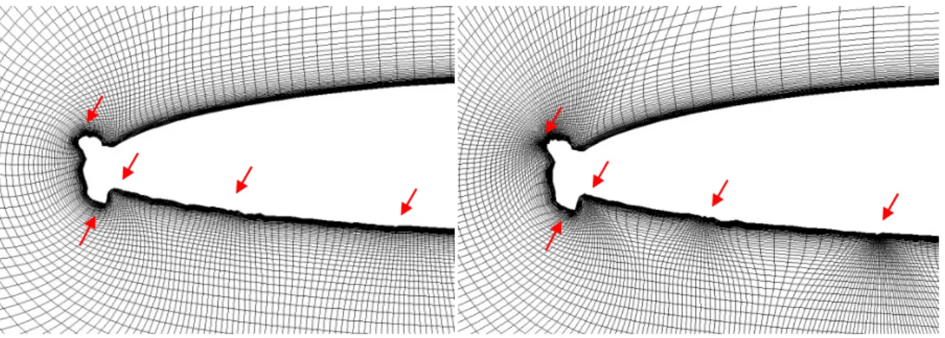
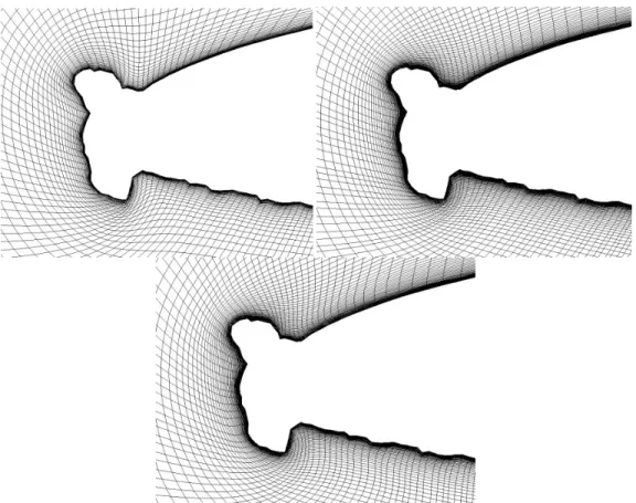
additional use of RANS information, namely the heat transfer parameters to the icing thermodynamic module (instead of the boundary layer method solution). The results of LEWICE-NS using the ICEG2D grid generation package for two case studies (rime and glaze ice) are shown in Figure 1.3. It is observed that the quality of the grid is not well preserved for the glaze ice case. Grid shocks, clustering/opening, smoothness and stretching are issues arising from simple parabolic method. The surface roughness effect has not been addressed in these results although it is an important criterion through the process of icing simulation as it influences the computed surface skin friction and heat transfer and results changes in ice accretion calculation [37].

Figure 1.3: Grid generated (rime ice [left] and glaze ice [right]) [12].

1.2.2 FENSAP-ICE

FENSAP-ICE is one of the first icing simulation codes developed within an Eulerian approach [36-38]. The code includes five main modules: an unstructured grid generation module, a finite element RANS based solver (FENSAP), an Eulerian based water droplet approach, a 3D ice accretion module, and Conjugate Heat Transfer (CHT) computation in presence of anti-icing heat transfer through the wing skin. The code uses unstructured or hybrid grids and applies grid deformation for multi-time step icing simulation (Figure 1.4) [14]. Uses of unstructured grids allow treatment of more complex geometries compared to structured based methods. Roughness effect has been studied by FENSAP-ICE through the use of rough wall treatment Boeing extension implemented in the Spalart-Allmaras turbulence module [37]. A Shallow Water Icing Model (SWIM) model is developed for the ice accretion and water runback computations, to complete the Messinger model. The code includes a hot air jet anti-icing module incorporated

(33)

with the thermodynamic computation through CHT module. The third generation of FENSAP-ICE-Unsteady has been developed to perform unsteady icing simulation [36].

Figure 1.4: FENSAP-ICE 3D ice solution [14].

1.3 Aerodynamic effects

It is known that an iced airfoil shows significant reduced lift and increased drag. This consequently results in stall at lower angle of attack compared to clean airfoils as well as decrease aircraft speeds [6, 39]. Glaze ice forms create a more destructive effect with large flow separation and early stall compared to rime ice forms. Generally, there are three ways to determine the icing effects on the airplane aerodynamic performances: 1) Flight testing; 2) Wind tunnel testing; 3) CFD simulations. These assessment methods differ in cost, simulation constraints for realistic test conditions, and modeling errors. Flight tests are very expensive, but they are the best way to have the most realistic conditions and results, although freestream conditions are not easy to characterize [4]. Wind-tunnel tests are less expensive albeit still out of reach of routine use, but they give additional flexibility to change and control tests conditions and icing parameters [7]. One drawback is the geometry scaling factor which significantly alters the results. The cheapest method is the application of CFD to model in-flight icing with a high flexibility to control the icing and flow conditions [6]. The accuracy of the CFD approaches depend on mesh quality, efficient turbulence models, boundary layer transition models, steady or unsteady simulations, etc. However, they can model flight test Reynolds number while aiding extrapolation of wind-tunnel results.

CFD methods help to determine proper trends with respect to the various parameters. RANS flow simulations can predict the flow behavior over simple ice shapes but lack sufficient

(34)

accuracy when ice shapes are more complex, such as those with large ice horns and very rough surfaces, or with unsteadiness effects. In these cases, there can be significant differences between the numerical predictions and the experimental results. In CFD analysis, grid sensitivity studies can be helpful to find the optimal grid properties for computation of the flow around the iced airfoil. The effects of grid quality and density can play a vital role when the analyses involve cases of high angle of attack or flow separation [40]. CFD methods need verification, as well as validation using experimental data. One of the major difficulties in validation of icing simulation codes is the availability of precise experimental data bases.

Measuring the ice shape by 2D cross sections has been so far as the most prefer method to obtain the experimental ice shapes data. Measuring ice shapes is very difficult because the ice surface includes large number of sharp edges, feathers, porosity and small size roughness. Also the ice deformation and melting can occur during the measurements. Covering the ice with paint or powders and using optical scanning is another method for measuring the ice shape, but it still has many difficulties and measurement errors [4, 7].

1.4 Thesis objectives

In view of the context described above, the overall goal of the work is to advance the numerical modeling towards advancing our understanding of the quasi-steady ice accretion process for complex ice accretion and aerodynamic effects.

In particular, the specific objectives are:

1- Examine the impact of RANS flow solver on the ice accretion framework. 2- Examine multi-steps ice accretion quasi-steady convergence.

3- Develop novel grid generation algorithms specifically for ice shape/growth.

Note that the research is centered around algorithms development, thus excluding studies of specific physical phenomena such as Supercooled Large Droplets (SLD) or non-uniform surface roughness effects. Also, although the framework is linked to both Lagrangian and Eulerian droplet formulations, only the Lagrangian approach is used in the thesis.

(35)

Towards the thesis objectives, the following platforms are used:

1) Polytechnique Montreal (PM) icing code, CANICE2D [15], based on Lagrangian formulation.

2) Polytechnique Montreal (PM) grid generation code, NSGRID2D&3D [41], (developed as a part of this research project).

3) ICEM-CFD commercial grid generation package [42]. 4) PMB3D RANS solver [43], University of Liverpool. 5) NSMB3D RANS solver [44], CFS Engineering Inc.

6) Polytechnique Montreal (PM) RANS solver, NSCODE2D [45].

The CANICE2D framework provides the starting point, with RANS capabilities inserted gradually in a sequential manner to finally obtain the CANICE2D-NS framework [20, 39, 46]. The developed framework then is used to generate a validation database and enable studies of icing effects on aircraft aerodynamics.

Note that the developments in NSCODE2D-ICE [34], NSGRID3D and icing framework of NSMB3D-ICE/NSGRID3D, published in ref. [47], are excluded from the content of this thesis. The thesis focuses on the development of two dimensional grid generation code NSGRID2D and RANS aero-icing framework CANICE2D-NS. The developed codes specifications are shown in Table 1.2.

Table 1.2: PM icing codes info.

Code Developer

Solver Specifications

Mesh Flow Droplet Ice

CANICE-NS (2D) Multi-steps PM NSGRID (Structured/ Elliptic Blended) RANS (PMB /NSMB /NSCODE) Lgrangian /Eulerian method Traditional Messinger NSCODE-ICE (2D) Multi-steps PM NSGRID (Structured/ Elliptic Blended) RANS

NSCODE Eulerian method Messinger Iterative

NSMB-ICE (2D/3D) Multi-steps PM/ Uni. de Strasbourg NSGRID (Structured/ Elliptic Blended) RANS NSMB Eulerian method Iterative Messinger

(36)

The thesis is organized as follows. Chapter 2 addresses the literature review, icing methodologies and algorithm developments. Chapter 3 addresses the consistency of the works and the publications toward the objectives of the project. Chapters 4 to 6 include the main publications, developments and discussion that address the three objectives of the thesis. A general discussion is presented in Chapter 7, before a conclusion in Chapter 8. Appendix A includes additional modeling descriptions. Appendix B includes additional NSGRID2D and CANICE2D-NS results and discussions.

(37)

CHAPTER 2 LITERATURE REVIEW AND METHODOLOGY

First the literature review is presented which includes: background in icing problem, the detailed description of traditional ice accretion process, and grid generation tools/methods survey for ice mesh generation problem. Finally the solution methodologies are addressed.

2.1 Background

2.1.1 Context

To reduce the number of incidents/accidents due to icing and enlarge aircraft certificates for flying in all weather conditions, one needs to develop icing simulation capabilities. Prediction of precise complex ice accretion resulting in aircraft performance degradation represents a challenge in aeronautical science. The National Transport Safety Board identified ice accretion and its effects as one of the major causes of flight accidents [1]. Ice forms on different surfaces of the aircraft, when flying in weather conditions with temperature lower or close to freezing point and with water droplets impaction on the aircraft surfaces. Ice can form with different characteristics categorized generally in three types of formations: rime, glaze, and mixed ice. The physical complexity of ice formations on glaze ice is higher than for rime ice. For instant, ice horns growth can lead to very odd shapes that cause higher flow disturbance and aerodynamic performance degradation [3].

In the field of ice accretion simulation, the traditional ice prediction simulation packages, such as LEWICE (NASA Glenn Research Center) [48], CANICE (Polytechnique Montreal) [18], are mainly based on potential flow solvers coupled with two dimensional boundary layer methods. The flow field solution is used to compute the water droplet trajectories and water collection efficiency on the aircraft via a Lagrangian approach, and also to compute the heat transfer coefficient needed for the ice accretion thermodynamic module [17]. Knowing the incoming water mass accumulation rate, water runback and heat transfer properties, the amount of accumulated ice is determined for a specific time period. Finally the surface geometry is updated using the amount of ice formed on the surface. Since, growth of ice on the body influences the flow field [31], the total ice accretion simulation is obtained by breaking the total icing time to

(38)

specific number of time steps, where each step is treated as a steady state flow problem (this approach is referred as multi-step procedure, using a quasi-steady approximation with each step). CANICE is an ice accretion simulation code developed at Polytechnique Montreal under research funded by NSERC and Bombardier Aerospace. The code includes four basic modules: external flow simulation, droplet trajectory and local catch efficiently calculation, surface ice/water interface thermodynamic balance and ice accretion and hot air anti-icing simulation (Figure 2.1).

Figure 2.1: CANICE code structure [2].

The CANICE2D code can perform for multi-element, multi-time steps icing simulations of airfoils. The flow solution is obtained by the Hess and Smith panel-method approach and is used for droplet trajectory and viscous boundary layer calculation. CANICE3D is the extension of CANICE2D to three dimensions, which has been integrated to CMARC, a low order three-dimensional panel method code, to compute the potential flow solution around the wing needed for the 3D droplet trajectories and impinging efficiency calculations [49, 50]. For both codes, a decoupled integral boundary layer or coupled viscous-inviscid interaction method is used to simulate viscous effects. To include the effect of roughness in the boundary layer model, the transition criteria, skin fiction and heat transfer calculation for laminar and turbulent region have been modified using roughness based empirical equations. Roughness is based on the equivalent sand-grain roughness height, which is calculated with an empirical model [15].

(39)

Droplet trajectory is simulated using the Lagrangian approach, solving the equation of motion of the water droplets for the defined time intervals using a forth-order Runge-Kutta scheme. The forces acting are the drag force on the spherical water droplets along with gravity and buoyancy force. The module thus determines the water droplet trajectories and impingement on the surface [49]. The droplet impingement distribution defines the water droplet local catch efficiency on the surface which determines the droplet mass flow rate impinged on the surface panels. Using the calculated local convective heat transfer and water droplet impingement flow rate on the surface panels along with runback water mass rate from the neighbor panels, the mass and energy balance is applied to the surface control volumes to calculate the amount of supercooled impinged water droplets converted to ice mass. The Messinger model is used to define the type of ice surface (wet, dry rime or wet glaze), freezing fraction (fraction of ice mass to the entering total mass flux to the control volume), and surface temperature [2, 11]. To take into account the hot air anti-icing heat flux, the anti-icing module solves the internal heat transfer coefficient using an empirical correlation related to impinging jet on flat plate. The correlation takes into account the average Nusselt number based on the jet parameters such as jet Reynolds number, nozzle to surface distance, and nozzle width [16]. Using the calculated internal hot-air local heat transfer coefficient and conduction through the thin leading edge skin, in an iterative process, wall heat transfer rate is calculated and integrated to the surface control volume thermodynamic balance. Final ice geometry is updated by calculating the ice height growth at the center of each panel and interpolating and smoothing the panel’s connectivity on the edges using panel size and angle criteria [51]. This step is not as easy as it appears, so a non-conservative method is used to simplify the process.

The panel method flow solver shows increasing errors in the flow solution as the complexity of the ice shapes increases, such as glaze ice with horns. The errors mainly comes from the higher influence of viscous effect and shows the need for RANS based flow solution for icing phenomena simulation and effects analysis [52]. The main difficulty of CFD based icing simulation comes from the point of grid generation for complex ice shapes, computation time and memory usage. New improvement in CFD based flow solution such as modified turbulence models with roughness effects, solution approaches for speeding up the convergence, parallel computing, unsteady flow solution, along with new developments in grid generation, smoothing and automation methods, have increased the efficiency of CFD based approaches in the ice

(40)

accretion simulation and effects analysis [53]. Note that CFD methods belonging to the class of Immersed Boundary Method (IBM), which considerably eases the grid generation problems of body-conforming methods, are not addressed here.

Grid generation methods, such as structured, unstructured, and hybrid grids, have been applied to icing problems [6, 14]. A finding of the NASA “CFD Vision 2030 Study: A Path to Revolutionary Computational Aerosciences” explicitly says “Mesh generation and adaptivity continue to be significant bottlenecks in the CFD workflow, and very little government investment has been targeted in these areas” [54], perhaps explaining the few developments in multi-block structured mesh generation algorithms in the last decades. Structured-grid methods suffer from the aspect of flexibility and grid quality for complex shapes such as ice accretion, but the flow solver is typically more efficient and accurate. The main difficulty of structured mesh in complex ice shapes domains is related to the grid smoothing approaches on physical domain boundaries which contain discontinuities, sharp angles, highly concave and convex area, etc. The process of grid generation for flow simulation on iced airfoils typically includes three basic steps: determination and smoothing of the iced surface; distribution of the grid points on the surface; and finally generation of the volume mesh using various approaches [23, 55]. There are three major classes for structured grid generation: algebraic methods, partial differential equation (PDE) methods, conformal mapping methods. PDE methods can be categorized as elliptic, hyperbolic and parabolic methods [23, 24].

PDE based methods such as elliptic Poisson equation (based on Laplacian operators), are solved by finite difference or finite volume discretizations to generate smoothed structured grids. They are more complex than algebraic methods but provide more flexibility to generate high quality grids using control functions. These methods use an algebraic grid generated as a starting grid (initial solution) and perform an iterative procedure to generate the desirable grid quality [22, 55]. There are still some difficulties using Laplacian operators, such as controlling grid spacing close to the wall or generating large cells in concave domain and small cells in convex regions. Control functions such as mesh spacing control, orthogonality control, and curvature control have been developed and used to increase the control on the generated grid quality. Spacing control functions modify the wall normal spacing and the stretching ratio of the grids. Orthogonality control functions modify the grid orthogonality and skewness throughout the domain. Curvature control functions modify normal spacing in concave/convex regions and grid

(41)

negative volumes [22, 56]. These grid controls, especially close to the wall for viscous dominated regions, have extensive influence on Navier-Stokes flow solution accuracy. It is thus important to have grids with good metrics, which are very difficult to obtain when geometries contain concave/convex domains with sharp corners [57]. A number of well known control functions developed by Sorenson, Steger, Thompson, Soni, and others, solve for spacing and orthogonality on the boundary and propagate the information throughout the domains using Laplacian operators [21, 23, 55]. Other control functions developed by Spekreije, solve the spacing, orthogonality and curvature using parametric space and impose the properties to the physical grid domain to retain the desired quality [22]. There are also methods to control grid quality such as boundary orthogonality approaches developed by Khamayseh, Kuprat through the use of specified Dirichtlet or Numann boundary condition in elliptic equation system of grids [23]. For the problem of ice, no elliptic method has yet produce adequate metrics, because of the complexity of the ice surface.

Conformal mapping approaches such as parabolic marching methods are another grid generation class discussed for the problem of ice grid generation. Thompson and Soni have developed an efficient parabolic grid generation code ICEG2D integrated to LEWICE and NPARC solver to perform multi-time steps ice accretion simulation [58]. The grid generation code is capable of surface and field grid generation and smoothing. The surface grid generation is done using a weight functioning based on the surface points. Also the surface is smoothed, to remove the sharp point complexity, prior using the parabolic approach. Surface is defined by NURBS functions. To develop the field grid, the code uses a conformal mapping approach and generates structured and semi-structured grids. Semi structured grids include quad and hexahedral elements. The structured grid approach includes two main steps: algebraically generation of locally orthogonal reference mesh and smoothing of the reference mesh using Poisson equation. To generate the semi-structured grid one need to add a third step: deletion and insertion algorithm based on the reference grid quality and defining the appropriate initial data surface for next layer generation. The efficiency of the method is addressed for icing aerodynamic performance simulation and analysis in reference [59]. Difficulties of structured parabolic grid rise from grid clustering and grid opening caused by concave and convex domains, respectively, and their propagation throughout the domain. The other issue is the nature of parabolic methods that are not well applicable for multi surface grid. In semi-structured grids,

(42)

the memory usage and the flow solver developments represent the main difficulties. These grids have unstructured data storage method and applications.

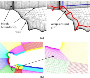
Some approaches and tools have also been introduced specifically for structured ice grid generation, and are mainly based on heuristics approaches. Shih developed an interactive tool to generate multi-block structured algebraic grid and block modification for ice grid problem [6]. The tool includes a large number of grid manipulation and modification applications on geometry, blocks, edges, domain grids, etc. The code also includes simple elliptic domain smoothing. To prepare the ice surface grid, first the ice geometry is smoothed to remove the complexity of the ice shapes with horns, sharp edges, feathers and surface roughness. Then to generate the field grid, one needs to define the blocking topology as single block or multi-block. Both blocking topologies result in some advantages and disadvantages to control the grid quality. Single block method includes two domain sections, a fine grid domain close to the ice shape that will be smoothed and a coarse grid domain in far field. The multi-block method includes a thick wrap-around section covering the ice shapes that minimizes the influence of ice geometry on the field grid. The rest of the domain is divided into as many numbers of blocks for better grid manipulation. Both single and multi-block methodologies are very time consuming and need extensive application by user. Automation of the methodologies is also an issue. The generated grids by these approaches have been used for different application of iced airfoil RANS based flow simulations.

Although there have been many proposed grid methods, CFD applications for icing simulations remain impeded by the absence of a robust grid generation process that results in high quality Navier-Stokes resolution grids for severe mixed concave/convex glaze ice shapes. The process of mesh generation in multi-time steps icing sequences can be performed via mesh regeneration or mesh movement (spring analogy [60], elastic [61], adjoint-based [30]). Although mesh movement is used by some researchers for icing simulations [58, 38], it has been found that, at least in 2D, the alternate approach of mesh regeneration provides increased robustness [13]. Automation of the grid generation process is another important aspect for performing multi-time steps icing simulations.

The other important aspect in CFD based icing simulation is the modeling and imposing the effect of roughness in ice accretion process as it highly influences the computed surface skin friction and heat transfer rate that results in changes in ice accretion determination [31, 37].

(43)

Surface roughness height generally is computed using empirical models such as sand-grain model [2] within boundary layer codes. To impose the effect of roughness for RANS based icing simulation, one need to implement the roughness effects in standard turbulence models. For this aspect, the rough wall treatment implementation in turbulence models such Spalart-Allmaras and k-ω models have been developed [26]. For the Spalart-Allmaras turbulence model, there are two extensions: the ONERA and Boeing models [27]. The roughness is incorporated to the S-A model by affecting the turbulent eddy viscosity in the wall region. One can relate the roughness height to the changes in velocity profile which changes the wall skin friction. Using two equations k-ω model, two rough wall models have been addressed: Wilcox method and Knopp method [28].

Generally the roughness value is assumed to be constant on the ice surface but in reality its value changes through time and space. There have been attempts to compute its value based on the water beading on the surface [62]. Based on the observed behavior of the impinging water on the surface, water droplets at first form small beads with spherical shape (because of the surface tension force). The beads start to grow as more droplets impinge the surface. Part of the bead freezes while the other liquid part covers the surface. As the beads grow in size, it finally reaches a maximum bead height and the water starts to flow on the surface due to the air flow shear force. The frozen part of the bead (ice bead) forms the surface roughness height which is taken equivalent as the sand grain roughness height and used in single and multi-time steps icing simulation [2, 63].

For the problem of icing droplet trajectory and impinging efficiency calculation, two approaches have been addressed: Lagrangian and Eulerian methods. In the traditional Lagrangian approach where the droplets are treated, the equations of motion for the droplet are solved to compute the droplet velocity and position in space through the time intervals [5]. The difficulties of the Lagrangian approach are its high computation time and collection efficiency calculation in complex domains. In the Eulerian approach, the droplet flow field is solved as a two-phase flow problem through the conservation mass and momentum equations [32, 33]. Solving the continuity and momentum equation for the water droplets provides droplets velocities and water volume fractions solution in the domain. The water droplets velocity is solved on the same mesh and nodes than the fluid and the water flux impinging on the surface is calculated directly [49, 64]. Different approaches such as FEM or FVM can be applied for discretization of the